www.atmos-meas-tech.net/2/533/2009/
© Author(s) 2009. This work is distributed under the Creative Commons Attribution 3.0 License.
Measurement
Techniques
Cloud detection for MIPAS using singular vector decomposition
J. Hurley, A. Dudhia, and R. G. Grainger
Atmospheric, Oceanic and Planetary Physics, Clarendon Laboratory, Department of Physics, Parks Road, Oxford, UK Received: 31 March 2009 – Published in Atmos. Meas. Tech. Discuss.: 29 April 2009
Revised: 7 September 2009 – Accepted: 8 September 2009 – Published: 18 September 2009
Abstract. Satellite-borne high-spectral-resolution limb sounders, such as the Michelson Interferometer for Passive Atmospheric Sounding (MIPAS) onboard ENVISAT, pro-vide information on clouds, especially optically thin clouds, which have been difficult to observe in the past. The aim of this work is to develop, implement and test a reliable cloud detection method for infrared spectra measured by MIPAS.
Current MIPAS cloud detection methods used opera-tionally have been developed to detect cloud effective fill-ing more than 30% of the measurement field-of-view (FOV), under geometric and optical considerations – and hence are limited to detecting fairly thick cloud, or large physical ex-tents of thin cloud. In order to resolve thin clouds, a new de-tection method using Singular Vector Decomposition (SVD) is formulated and tested. This new SVD detection method has been applied to a year’s worth of MIPAS data, and qual-itatively appears to be more sensitive to thin cloud than the current operational method.
1 Introduction
Clouds are increasingly recognised for their influence on the radiative balance of the Earth and the implications that they have on possible climate change, as well as in air pollution and acid-rain production. However, clouds remain a major source of uncertainty in climate models. High thin clouds such as cirrus are important to study.
High clouds are frequently observed at all latitudes and, at any one time, 60% of the Earth’s surface is covered by cirrus (Wylie et al., 2005). High clouds are important be-cause they are high enough to act to warm the Earth; how-ever this mechanism is not well understood in terms of the
Correspondence to:J. Hurley ([email protected])
relation of micro- and macro-physical cloud properties. Be-cause they are so wide-spread and permanent, it is impor-tant to understand how these clouds affect the climate. How-ever, current cloud detection algorithms often miss much thin cloud in satellite measurements, and the instrumentation it-self (eg. nadir versus limb, microwave versus infrared and so on) specifies varying thresholds of senstivity to different cloud types – and hence conventional cloud climatologies and inventories are incomplete with respect to high thin cloud such as cirrus (Wylie et al., 2005).
There have been many studies on clouds over the years and many climatologies: by Barton (1983), Warren et al. (1985), Woodbury and McCormick (1983), Prabhakara et al. (1988), Wylie and Menzel (1989), Wylie et al. (1994) – but these were all limited by a lack of global coverage. Currently, the Stratospheric Aerosol and Gas Experiment (SAGE) (e.g. SAGE, 2002), High Resolution Infrared Radi-ation Sounder (HIRS) instrument (e.g. Wylie et al., 2005), International Satellite Cloud Climatology Project (ISCCP) (e.g. ISCCP, 2008) and GRAPE project (e.g. Sayer et al., 2009) are actively compiling cloud climatologies.
2 Overview of MIPAS-ENVISAT
The Michelson Interferometer for Passive Atmospheric Sounding (MIPAS) is an infrared limb-viewing instrument and was launched in March 2002 on the European Space Agency’s Environmental Satellite (ENVISAT). ENVISAT is in an 800 km sun-synchronous polar orbit, with a nominal orbit having a repeat period of 35 days, an orbital period of 100.6 min and an inclination of 98.54◦. The inclination of the orbit in conjunction with azimuth scanning enables full global coverage pole-to-pole (ESA, 2005).
and NO2) at a high spectral resolution in the near- to
mid-infrared from 685 cm−1 to 2410 cm−1 in five discrete
bands (A 685–970 cm−1, AB 1020–1170 cm−1, B 1215–
1500 cm−1, C 1570–1750 cm−1, and D 1820–2410 cm−1). In its initial operating specifications, MIPAS operated at a spectral resolution of 0.025 cm−1, measuring spectra nomi-nally every 3 km vertically in the troposphere – however fol-lowing persistent slide malfunctions in early 2004, the res-olution was decreased to 0.0625 cm−1but the measurement tangent height spacing decreased to nominally every 1.5 km in the lower stratosphere and troposphere (Mantovani, 2005). The FOV of MIPAS is approximately 3 km high and 30 km horizontally, perpendicular to the instrument line-of-sight. The FOV is modelled by a trapezoidal response function φ (z), having a 4 km-high base and a 2.8 km-high top.
3 Current detection methods for MIPAS
The presence of cloud particles in the FOV of infrared remote sounding instruments influences observations registered, due to extraneous absorption, emission and scattering features in a large range of wavelengths. Clouds in the line-of-sight can act as grey-bodies with significant opacity which alter the measured radiation, and introduce serious problems in sensing atmospheric temperatures and gas profiles below the cloud level. All clouds cause a broadband increase in the radiance emitted and measured in the FOV – however thin clouds also introduce a multiple-scattering effect which im-plies that the instrument measures radiance from below the tangent height. The presence of clouds introduces problems with regular constituent retrievals by introducing a sharp transition from optically thin to optically thick limb trans-mittance at the cloud top. In order to avoid this, and to main-tain retrieval quality/reliability, routine processing of MIPAS spectra includes the detection and rejection of all spectra with significant cloud contamination. However, studying these cloud-contaminated spectra can reveal information about the cloud itself.
The following sections outline the detection methods which have been either proposed or operationally used to de-tect cloud in MIPAS measurements.
3.1 Mean Radiance Thresholding and Colour Indices
A very basic method is the Mean Radiance Threshold test which simply uses a statistically gathered radiance thresh-old to detect cloud by assuming that clouds have a warmer brightness temperature than a clear limb view. For MIPAS, considering the region around 960.7 cm−1a radiative transfer model, the Reference Forward Model (the RFM, a GENLN2-based line-by-line radiative transfer code originally devel-oped to provide reference spectral calculations for MIPAS by Dudhia, 2005), is used to simulate the transmittance spec-trum – and the 960.7 cm−1region is used as it has high
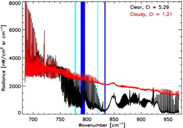
trans-Fig. 1. Samples of clear (black) and cloudy (red) MIPAS spectra with the locations of the current CI MWs (blue) and optimised CI MWs (aqua) overplotted.
mission and low gaseous emission. Thus, in order to de-tect a cloud having an extinction coefficient of 10−4km−1,
a threshold of 100 nW (cm2sr cm−1)−1must be chosen at a
tangent height of 9 km (higher threshold for lower tangent heights and for higher extintion values).
A second generation detection method is Colour Index (CI) Thresholding (Spang et al., 2004). CIs work on the prin-ciple of radiance ratios between two different regions (called microwindows MWs, and denoted MW1 and MW2) of the spectrum which respond differently to cloud. The MWs are chosen such that the first microwindow MW1 responds very little to the presence of clouds whereas the second microwin-dow MW2 shows a large reaction, as shown in Fig. 1. Use of a ratio of radiances from each measurement spectrum im-plies that the variability in radiance resulting from temper-ature and pressure fluctuations is effectively cancelled out, since both sections of the spectrum will scale consistently to such changes – and hence thresholds can be more reliably picked.
The CI is defined to be the ratio of the mean radiances of the two MWs:
CI= ¯ LMW1 ¯ LMW2 . (1)
When CI is large (CI>4, for conventionally chosen MWs, MW1=792–796 cm−1 and MW2=832–834 cm−1), cloud-free conditions exist and when CI is approximately unity op-tically thick clouds are present. The range of CIs represents the range of optical thickness of clouds present, with thicker clouds appearing blackbody-like with CI≈1 and thinner, ten-uous clouds registering increasingly larger CIs.
only conservatively discarding data which are truly contam-inated by thick cloud, a low threshold is frequently chosen, below which it is certain that cloud occurs and above which cloud is said to not occur, even though it is well known that above this threshold cloud can indeed occur, either as an op-tically thin cloud or by only partially filling the instrument FOV. In operational processing for MIPAS, this threshold is set at CI=1.8 (Spang et al., 2004; Ewen, 2005).
It should be noted that the definition of CI breaks down above about 30 km due to decreased signal-to-noise-ratio, particularly in the more transparent and intrinsically noisier (due to smaller signal) second MW. Cloud detection itself gives a measure of the cloud top height, but this is limited to the height resolution of the measurement scan pattern.
3.1.1 Analysis of current operational CI detection method
A useful quantity to measure the amount of cloud present in a measurement FOV is the cloud effective fraction (EF), as defined by
EF=
Rzct
−d 1−e−kextx
φ (z)dz
Rd
−dφ (z)dz
(2)
for a FOV of width 2d characterised by the FOV function φ (z)corresponding to integrated pencil beam radiances each penetrating a pathlength x through an atmosphere of ex-tinction coefficientkextand cloud top height zct relative to
the tangent height. It is essentially the effective blocking power of the cloud within the FOV – the proportion of the FOV filled by cloud modified by the extinction of the cloud. Therefore, an EF=0 indicates that a measurement is cloud-free or “clear”, an EF=1 represents a FOV that is completely filled with thick cloud and 0<EF<1 represents the spread of varying cloud-filled states of a FOV.
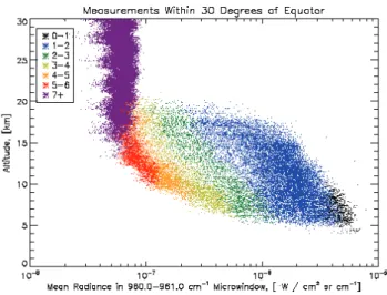
It can be asserted that the CI Method used operationally fails to detect many cloudy FOVs – as well as incorrectly di-agnosing clear spectra as cloudy. Considering the average radiance measured in the 960.0–961.0 cm−1 MW (a region of the A band spectrum having comparatively high trans-missivity – which implies that most variations in radiance come from continuum features, such as induced by clouds) as shown in Fig. 2 (with different values of CI assigned different colours), there exist two distinct regions, one corresponding to cloudy measurements and the other to clear measurements. The leftmost region is a thick band extending through all al-titudes at relatively low radiances, which represents the clear measurements. To the right of this thick band is a scattering of radiance points, starting at an altitude that could be taken as the maximum average tropopause height, at higher radi-ances – these points represent the cloudy measurements. The spread in these cloudy radiances is a result of many possi-ble fractions of cloud experienced by the measurement FOV. The present MWs and threshold used for cloud detection do
Fig. 2. Average radiance profiles measured in the 960.0– 961.0 cm−1MW by MIPAS, whereby the measurements have been assigned colours to indicate their CI value.
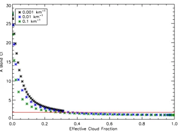
not detect the measurements which through this analysis are obviously cloud-contaminated (i.e. spread to the right of the thick band of clear measurements), although with a small EF. It is interesting to note that increasing the value of the thresh-old to a higher value of CI (than the currently used 1.8) does have the effect of picking up this scattering of cloudy cases, but that it also results in the clear cases (those measurements occurring in the thick leftmost band) being flagged as cloud as well. Fig. 3 shows that for EF less than about 0.3, the CI Method with the current threshold of 1.8 is not able to detect cloud at all. Altitude-dependent thresholds would partially solve the problem of misdetection, however given the inclu-sion of clear spectra as cloudy as a consequence of emisinclu-sion by water vapour, the CI method has key caveats which cannot be rectified by simply setting different thresholds.
Furthermore, there is a known problem with the CI method whereby clear spectra are misdiagnosed as cloudy, deriving from the fact that water vapour emissions in the lower at-mosphere can create broadband continua features, much like those exploited in the CI method itself (Spang et al., 2004).
Given the relative insensitivity of the current operational cloud detection method to optically thin cloud or of FOVs only partially covered in cloud, as well as its sensitivity to water vapour emissions in the lower atmosphere, there appears to be room for development of a cloud detection method which is capable of reliably resolving and identifying even these small amounts of cloud in measurements.
3.2 Singular Vector Decomposition
Fig. 3.Relation between cloud effective fraction and CI for RFM-simulated clouds with extinction coefficients of 0.001–0.1 km−1in the MIPAS A band. The red line shows the CI threshold (1.8) below which cloud is detected.
variables into a smaller number of uncorrelated variables called singular vectorsv. The first singular vector v0 ac-counts for as much of the variability in the data as possible, and then each successivevi accounts for as much of the re-maining variability as possible.
Consider anm×nmatrixL(Press et al., 2007). In this ap-plication,Lis a set ofmspectra each of lengthn– and each spectrum of lengthnis denotedl). Then,Lcan be expressed as
L=WTSV (3)
wherebyVandWare them×nandm×morthogonal matri-ces containing left- and right-singular vectors, respectively, andS is am×mdiagonal matrix whose diagonal elements contain themsingular valuesSi. The singular values (S) are
essentially eigenvalues corresponding to the singular vectors (vs), which are analogous to eigenvectors. Hence, the orig-inal matrixLis merely a linear combination of the singular vectors as scaled by the singular values (Murtagh and Heck, 1987).
Application of the decomposition yields a set (V) of a maximum ofmsingular vectors (vs) each of lengthnwhich best orthogonally span the variance of the initial ensemble of measurements (in the sense that thevs can then be thought of as a set of basis vectors inRn chosen so that the maxi-mum object-to-object variation in the data belongs to a sub-space formed by the least number of basis vectors). Thevs are usually ordered (by choice) by decreasing magnitude of their eigenvalue. Thus, each successivev captures increas-ingly less and less information, such that the percentage of the total variancePi captured by theithvis
Pi =
di
Pm
i=1di
×100%. (4)
The original input measurementsLij can be reconstructed
simply by calculating the appropriate linear combination of thevsand their corresponding singulars values, as described by
Lij =WTikSklVlj (5)
whereLij is thejth spectral measurement of the ith
spec-trum fori ǫ[1, m]andj ǫ [1, n]. In this notation, summa-tion occurs over the indiceskandl, wherek ǫ[1, m]andl ǫ[1, m]. Since the first fewvscapture so much of the total variance of the dataset, it is often sufficient to only sum over the first few singular vectors (for example, not from 1 tom, but rather from 1 to 2 or 3) in order to obtain a reconstruction which is good to within a few percent of the full reconstruc-tion.
The objective of this work is to use SVD techniques to create, implement and validate a reliable cloud detection method. The idea is to create an ensemble of simulated MIPAS spectra (Sect. 4) which contain varying amounts of cloud (because the EF characterising each spectrum will be known for simulated spectra) and then to use this ensemble to obtain singular vectors which correspond to the clear and cloudy atmospheric states (Sects. 5.1–5.2). Once the two or-thogonal sets of basis vectors (clear and cloudy) are known, any atmospheric signal should be able to be fit using both sets of vectors, regardless of whether the atmosphere is clear or cloudy (Sect. 6). By using some appropriate parameter related to the fitting process, it should be possible to create a cloud detection method (Sect. 8). Finally, this SVD-based cloud detection method will be compared with the current cloud detection method on a year’s worth of MIPAS data (Sect. 8) as well as using a set of simulated data for which the clear/cloudy state is known (as introduced in Sect. 4). It is hypothesised that the increased information gained by us-ing large regions of spectra (such as would be done for SVD-based methods) should lead to more reliable cloud detection than those based upon mean-continuum recognition (such as the CI method). Theoretically, it should avoid the misdetec-tion of regions of high water vapour concentramisdetec-tion as cloud, a caveat of the CI method, as the water-vapour continuum fea-tures should be well represented in clear atmospheric spectra used in the development of clear basis vectors – however this hypothesis has not been extensively tested in this work.
4 Ensemble of simulated clear and cloudy MIPAS spectra
The RFM was used to simulate an ensemble of spectra with varying amounts of cloud (as defined by their extinction co-efficients (kext) and cloud top heights (CTH)) occurring in
Table 1.Parameters used to create ensemble of cloudy atmospheres. Reference atmospheres compiled by Remedios (2001).
Tangent Height [km]
kext [km−1]
Reference Atmosphere CTH relative to Tangent Height[km]
6, 9, 12, 15, 18, 21 0.001, 0.01, 0.1 standard mid-latitudinal, tropical, polar summer and polar win-ter reference atmospheres, their one standard-deviational vari-ants, and separate perturbations in temperature, pressure, water vapour and ozone of each
−2.0,−1.5,−1.0, −0.5, 0.0, 0.5, 1.0, 1.5, 2.0
spectral features. The advantage of having an artificially cre-ated ensemble of spectra to examine as opposed to real data is that all of the cloud parameters are known in advance and one can without question identify with confidence different cases and regimes. The parameters used to build this ensemble of spectra are given in Table 1. In total, the ensemble has 5184 different atmospheric conditions: 576 of which are totally clear (i.e. cloud top height =−2.0 km) and 4608 of which which contain some finite amount of cloud in the correspond-ing MIPAS FOV (here, when cloud top height>−2.0 km). These simulations have been carried out at the MIPAS full-resolution of 0.025 cm−1in the second half of the MIPAS A band (827.5–970.0 cm−1, 5701 spectral points).
It should be noted that the RFM is a non-scattering model – and hence produces simplified spectra, as real clouds will have both single and multiple scattering features, as well as the broader features reproduced by the RFM. Hurley (2008) used single-scattering simulations to quantify the discrep-ancy between non-scattering and more-realistic scattering simulations – and found that for clouds having extinction co-efficients larger than 10−4km−1, the difference was
negligi-ble.
5 Calculation of singular vectors
In the following SVD studies, the ensemble discussed in Sect. 4 is separated by tangent height, and data from each tangent height are treated independently. Since, in practise, the nominal tangent height is a well-known discrete param-eter of MIPAS data, this segregation has been carried out in order to preserve vertical atmospheric variations which con-sistently occur.
SVD has been carried out by first dividing the ensemble of spectra into two regimes: clear (EF=0) and cloudy (EF6=0). Then each of these two atmospheric regimes is sub-divided into smaller ensembles grouped by tangent height. To nor-malise the data, each spectrum in the ensemble has had its av-erage radiance subtracted (which effectively allows clear and cloudy singular vectors to share reconstructive responsibility of the raised cloud radiance baseline – otherwise the clear singular vectors are simply forced to accommodate more of the radiance coming as a result of the cloud presence, see
Hurley (2008) for details), and then SVD is carried out upon each of the normalised tangent height ensembles.
5.1 Clear singular vectors
Using the clear ensemble of spectra, divided by tangent height and normalised, SVD is carried out to calculate the clear singular vectorsvclear
i. For a tangent height of 9.0 km,
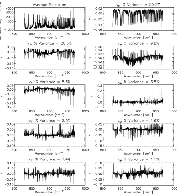
Fig. 4 shows the average clear spectrum for the 9.0 km clear ensemble along with the first eight singular vectors. It should be noted that the zeroth ordervclear carries so much of the variance associated with the ensemble that it visually resem-bles the average spectrum, while the higher ordervclearspick up more non-trivial variances, which is expected due to the large range of variations in clear atmospheric spectra due to local changes in pressure and temperature. If the total vari-ance captured by the addition of each successivevclearin the decomposition is considered, the first three vclears contain over 80% of the total variance. Thus, the SVD method effec-tively minimises the number of pieces of information needed to represent a set of data, since any of the initial pieces of information (here, the spectra) can be reconstructed by using as few as three singular vectors.
5.2 Cloudy singular vectors
Considering now the second ensemble of spectra which con-sist of simulations of infrared measurements containing some finite amount of cloud, the component of the signal which is due to the cloud alone is sought. The measurement regis-tered by the instrument FOV will be some combination of emission and absorption from the clear atmospheric com-ponents (ie. the gases) and those resulting from the cloud presence. The singular vectors obtained for the clear ensem-ble of spectra should represent the clear component in these mixed clear/cloud measurements and by using these already obtainedvclears, the component due to the cloud alone can be retrieved. The basis of this work is the hypothesis that a cloud-contaminated spectrum can be decomposed into com-ponents coming from the clear atmosphere and those due to the cloud itself.
Fig. 4.Average clear spectrum for the 9.0 km clear ensemble along with the first eight singular vectors and the percentage variance captured by each.
atmospheric contribution along with that coming from the cloud itself) in the cloudy tangent height ensemble is first normalised by subtracting off its average radiance to give lcloudy+clear
norm =lcloudy+clear− ¯lcloudy+clear (6) the component due to the clear background atmosphere can be obtained by carrying out a linear least squares fit using the clear singular vectorsvclear
i such that the clear radiance
componentlclearof the measurement is
lclear=
m
X
i=1
λivcleari (7)
whereλi are fit coefficients. Since the fit of the normalised
signal by the clear singular vectors will have captured any of the variance due to the clear sky, it is necessary merely to subtract to obtain the cloudy component of the signal (lcloudy):
lcloudy=lcloudy+clear
norm−lclear. (8)
Carrying out this procedure for each cloudy spectrum in each tangent height ensemble yields an ensemble of spectra regis-tering only the cloudy component for an abundance of cloudy atmospheric conditions. SVD can then be performed on this cloud-signal-only ensemble to yield a set of cloud singular vectors vcloudy
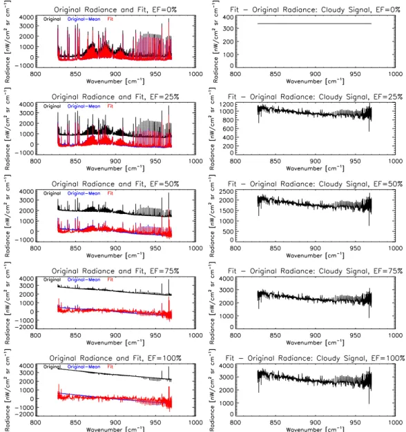
Fig. 5.Fitting of cloudy signal by clear singular vectors to obtain cloud-only signal component for cloud in a 9.0 km TH FOV. From top to bottom of the plot, EF increases in equal increments of 25% from 0% to 100%. Left panels: the original signal containing varying amounts of cloud is shown in black, the normalised original signal in blue, and the clear singular vector least squares fit in red. Right panels: the component of the original signal caused by the cloud as calculated in Sect. 5.2.
vectorsvclear
i. Figure 5 shows how cloudy measurements of
varying EF between 0 and 1can be individually fitted by first normalising the input radiance and then applying the linear least squares fitting invclear
i. It bears noting that the
non-zero difference between the linear least squares fit and the original signal is due to the removal of the mean radiance, as expected, and carries no spectral information.
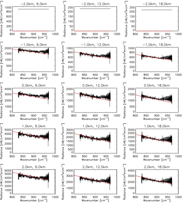
The residual cloudy signal reported is a complicated spec-trum with many emission and absorption features which de-viate from that of a blackbody at the appropriate cloud top temperature. However, Fig. 6 shows these cloudy signatures
Fig. 6. The cloud-only signal component of original partially cloudy measurement. From top to bottom of the plot, EF increases in equal increments of 25% from 0% to 100%. From left to right, the TH of the FOV containing the cloud is increased from 6.0 km to 12.0 km to 18.0 km. Blackbody-only signature is overplotted in red and shows good agreement with retrieved cloud-only component of signature given in black.
6 Fit an arbitrary cloud signal with singular vectors
Using the previously calculated clear and cloudy singular vectors, vclear
i and vcloudyi (of which there are mclear and
mcloudy, respectively), for each MIPAS tangent height where
cloud is normally expected, any measured MIPAS spectrum in the spectral range of 827.5 cm−1to 970.0 cm−1can be ac-curately fitted by a linear least squares fit in the singular vec-tors. Taking an arbitrary MIPAS spectrumlorig, the first step is to normalise the spectra by subtracting its average radiance
(as explained previously) such that
lnorm=lorig− ¯lorig. (9)
The linear least squares fitlfitoflnormis then trivially found, such that
lfit=
mclear
X
i=1
λclearivcleari+
mcloudy
X
i=1
λcloudyivcloudyi, (10)
whereλcleariandλcloudyiare constant coefficients of the least
compared with the original input measurement, it remains simply to add back on the constant average radiance of the original signal to the fitted spectra:
lfit orig=lfit+ ¯lorig. (11)
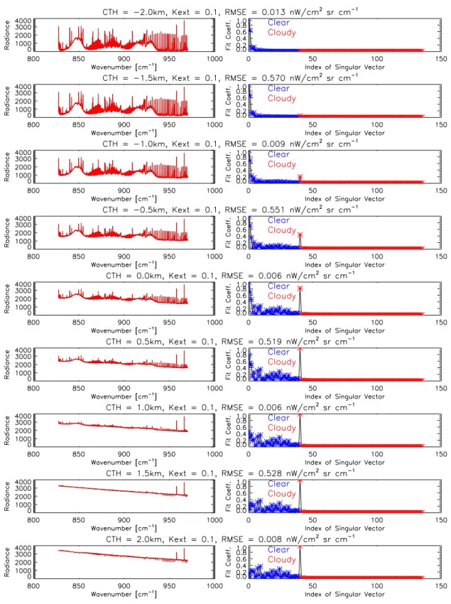
This method was implemented and tested on RFM-simulated spectra for infrared spectra with a tangent height of 9.0 m and extinction coefficients between 0.001 km−1and 0.1 km−1and cloud top heights located every 0.5 km in the 4.0 km-wide MIPAS FOV. Figure 7 shows the efficiency and consistency with which the linear least squares fit using both the clear and cloudy singular vectors is able to fit a signal with an arbitrary amount of cloud in it for a tangent height of 9.0 km and extinction coefficient of 0.01 km−1. It is also interesting to note that as increasing amounts of cloud are added to the measurement, the fit coefficients corresponding to the cloudy singular vectors increase in magnitude (partic-ularly that corresponding to the first cloudy singular vector, those of the next first few singular vectors which are non-negligble, but an order or magnitude smaller than that of the first), while those corresponding to the clear singular vec-tors decrease in magnitude. This is an encouraging trend, since it is expected that if there is increased cloud presence in the measurement, the signal should be increasingly well fit by the cloudy singular vectors with a minimised dependence upon the clear singular vectors.
This method was then applied to a scan of apodised MI-PAS spectra, which has been flagged as cloudy by the CI Method in the final sweep at 6.0 km but clear everywhere above. Figure 8 shows the fits of the input raw spectra over-laid with the fit obtained from the clear and cloudy singular vectors, which clearly do a good job of fitting the signal since the root mean square error is less than 1.0% of the measure-ment’s spectral baseline. As well, it is obviously the clear singular vectors which dominate fit until the final sweep, at which the cloudy singular vectors are fitted with non-zero fit coefficients, corresponding well to the present cloud detec-tion mechanism’s judgement of the cloudy state of the atmo-sphere in that sweep only.
Given the success in reproducing spectral features through fitting with the clear and cloudy singular vectors as well as the fact that the clear and cloudy singular vectors are used in relation to each other in a manner which is expected, for both simulated and real MIPAS data in the spectral region consid-ered, it appears as if this method should be able to be used to detect and quantitatively determine the amount of cloud occurring in the MIPAS FOV.
7 Effect of noise on singular vector fits
It is interesting to consider how the SVD fit of a noisy signal (such as obtained from real measurements) will differ from that of a noise-free signal. In other words, the way in which the singular value assigned to each noise-free singular vector
in the fitting process is affected by noise on the input spectra is sought.
Consider a noise-free radiance spectrumlof lengthnsuch that
l= l1, l2,· · ·, ln (12)
which is to be fit by a singular vectorvof lengthnwhere v= v1, v2,· · ·, vn. (13)
Then the least squares linear fit of the spectrum using the singular vector can be expressed as
λ=vTv−1vTl. (14) It immediately follows that
λ=(v·v)−1vTl=(|v|)−1vTl=vTl (15) since|v| =1 becausevis a unit vector by nature. Discretising this yields
λ=
n
X
i=1
vili. (16)
If random noise of amplitudeσ is added to each spectral point on this arbitrary spectrum, there will be some change σλin the singular value assigned by the least squares fit. The
least squares fit to the noisy spectrum can be expressed as λnoisy=λ+σλ=
n
X
i=1
vi(li+σi) . (17)
It follows that σλ2=
n
X
i=1
(vi)2σ2=σ2 n
X
i=1
(vi)2=σ2 (18)
sincePn
i=1(vi)2=1 asvis a unit vector. Hence the fit
coef-ficient to the noisy spectrum is simply
λnoisy=λ+σ. (19)
For MIPAS, σ=50 nW (cm2sr cm−1)−1 1. Typical fit co-efficients for the first few singular vectors in both the clear and cloudy sets (i.e. those important to the fit, as they represent the largest variances) are of the order of 10000 nW (cm2sr cm−1)−1– so the change in the fit
coeffi-cient (λnoisy−λ=σ) is minor for mostλsinceλ≫σ for most vs. Thus, the difference caused by the presence of this max-imum value of noise is negligible.
Therefore, random error on the input measurements should not greatly affect the fitting of the spectra by noise-free singular vectors as the vectors important in the fitting mechanism are negligibly changed by the noise.
1This is an overestimation of the effect of noise, since Eq. ( 18)
Fig. 8.Fitting of MIPAS spectra by clear and cloudy singular vectors. From top to bottom, downwards through the scan pattern: 15.0 km, 12.0 km, 9.0 km and 6.0 km tangent heights. Left panels: linear least squares fit using both clear and cloudy singular vectors (red) overplotted on original input signal (black). Right panels: magnitudes of fit coefficients corresponding to the singular vectors used in the fit (clear in blue, cloudy in red), normalised such that the largest fit coefficient has a magnitude of unity.
8 SVD cloud detection method
As described in the previous sections, using the set of clear and cloudy singular vectors should yield a cloud detection mechanism. This section will introduce and test a possible candidate for detection mechanism which reconstructs the portion of radiance that the fit attributes to a cloudy presence. Any arbitrary spectrum can be successfully fit to a high degree by a set of altitude-dependent singular vectors which span the clear and cloudy atmospheric states such that
ltotal=
mclear
X
i=1
λclearivcleari+
mcloudy
X
i=1
λcloudyivcloudyi, (20)
in keeping with standard reconstruction of SVD, as discussed in Eq. (5), whereλcleari andλcloudyi are constant coefficients
of the least squares fit. Once this linear least squares fit has been obtained, it is trivial to reconstruct the radiance compo-nents of the original signal: that due to the clear background
state and that due to possible cloud presence. Reconstruct-ing, the clear radiance is
lclear=
mclear
X
i=1
λclearivcleari, (21)
and the radiance due to the cloud presence is lcloudy=
mcloudy
X
i=1
λcloudyivcloudyi. (22)
It follows, then, that when the radiance due to cloud pres-ence becomes non-zero, cloud is present. To normalise this quantity, the ratio of the cloudy radiance to the total radi-anceLtotal, called the Integrated Radiance Ratio, is
consid-ered such that
¯
Lcloudy
¯
Ltotal
>0 (23)
for cloudy spectra and
¯
Lcloudy
¯
Ltotal
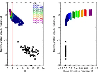
Fig. 9.Integrated Radiance Ratio for all RFM-simulated spectra in ensemble plotted as a function of CI (left panel) and EF. Colour-coded by EF.
for clear spectra, whereL¯ represents the average of the re-constructed radiancel in the 960–961 cm−1 MW. It is
hy-pothesised that this ratio could be used as a cloud detection method.
The ensemble of RFM-simulated MIPAS spectra has again been used to test this hypothesis. Following the least squares fitting of each spectrum with the altitude-corresponding set of clear and cloudy singular vectors, the cloudy radiance is reconstructed as previously described, the average in the 960–961 cm−1region calculated and the Integrated Radiance Ratio determined. When the ratio is plotted against CI or EF, as shown in Fig. 9, it becomes obvious that this hypothesis is valid, as the ratios form a bimodal distribution corresponding to clear and cloudy cases.
Thus, the Integrated Radiance Ratio is calculated for all MIPAS spectra measured for the full year of 2003 between 60◦S and 60◦N. To confidently choose thresholds, it is a matter of fitting the clear peak in the bimodal distribution to a Gaussian distribution – however this is not a trivial proce-dure since above the clear distribution maximum, there will be non-negligible cloud cases from the tailing edge of the cloudy portion of the overall distribution. Therefore, in fit-ting the clear distribution, only points in the distribution oc-curring to the left of the peak are considered. Furthermore, the thresholds are altitude-dependent and will be assigned for each unit altitude between 6.0 km and 21.0 km. In this man-ner, probability distributions functions corresponding to each unit altitude between 6.0 km and 21.0 km are considered and the “clear” peak (that centred the furthest to the left) fitted by a Gaussian distribution and the altitude-dependent threshold set at
Thr(z)=µ(z)+3σ (z), (25)
for the peak maximum µ and standard deviation σ. Fig-ure 10 shows the PDFs, overplotted with the clear peak fit withµandσ noted. It is reassuring to note that at the higher considered altitudes, the cloudy peak in the bimodal distri-bution becomes negligible with infrequent cloud expected. It should be noted that the thresholds thus chosen for the low-est altitudes should be treated with some care, as there is sig-nificant overlap between the clear-and-cloudy distributions which may not be fully isolated in the estimation of thresh-olds.
9 Application to MIPAS data
This SVD detection method, with the previously derived thresholds, is applied to all available MIPAS data from 2003, as shown in Fig. 11. It appears that this Integrated Radiance Ratio cloud detection method does a good job in identify-ing even the thin cloud that the present CI Method appears to miss, choosing all points to the right of the thick clear band in Fig. 11 as cloud – and thus to a first order, it appears to do better than the existing CI Method in terms of identi-fying cloud. The SVD method suggests that there are 28% of scans having cloud occurrence somewhere in the altitude range ubiquitous with high cloud (6–24 km), comparing well with Wylie et al.’s (2005) result which records high cloud in 33% of measurements taken (the CI method sees only 17% of scans as cloud-filled, with its current thresholds).
It is important to note that detection methods are highly sensitive to choice of threshold, although the choice of threshold is an imminently important component of the de-tection method itself. It could be argued that the operational CI method has been developped to identify thick cloud in or-der to avoid spurious trace species retrievals, and hence the operational thresholds are not tailored to isolate thin cloud, whilst the SVD method has been so developed. Exten-sive comparisons of the two methods are available in Hur-ley (2008) but have not been presented here for the sake of brevity (employing simulated clear and cloudy MIPAS spec-tra, as well as real MIPAS specspec-tra, using a wide-range of tests with-and-without the application of thresholds in order to examine the intrinsic skill of detection of the methods).
10 Application to polar stratospheric clouds
Fig. 10.Altitude-dependent PDFs of logLLcloudy
total
Fig. 11. Profiles of average radiance in 960.0–961.0 cm−1MW from all MIPAS spectra taken in 2003, between 60 S and 60 N. Left panel indicates in red those cases flagged as cloud by the CI Method. Right panel indicates in red those cases flagged as cloud by SVD Integrated Radiance Ratio Method.
this work is indeed to use this database to define basis vec-tors specific to PSCs, and to perhaps extend this detection method to differentiate between PSC types – a preliminary study of which was carried out in Hurley (2008) using real MIPAS PSC spectra.
11 Conclusions
SVD has been applied to an ensemble of simulated spec-tra which represent a large number of atmospheric states, both clear and cloudy. Singular vectors have been calculated which span both clear and cloudy atmospheres – and a cloud detection method (Integrated Radiance Ratio) has been for-mulated and tested, exploiting statistics of linear combina-tions of the two sets of singular vectors to represent any spec-tra encountered. Appropriate thresholds have been chosen by application to MIPAS data from 2003, and the methods qual-itatively tested on MIPAS data from 2003.
It appears that broadband spectral information can be ex-tracted by SVD and used reliably to detect cloud. The true success of this analysis lies in the apparent improvement that the SVD detection method seem to have over the op-erationally used CI method in the detection of thin cloud.
Simulated spectra have been used in the development of this analysis, which, arguably may not represent all of the possible clear atmospheric states – nor all the cloudy iter-ations. An interesting exercise would be to form singular vectors from real MIPAS spectra, however this poses the dif-ficulty of not knowing whether or not a singular vector cor-responds to the clear atmosphere, or to a cloudy one. Whilst there may be bifurcations in the appropriate distributions of
singular values, this is likely not a trivial task. In any case, the simulated singular vectors appear to do a good job at rep-resenting the real atmosphere – and the suggested detection methods seem to pick up both simulated cloud and what is hypothesised to be cloud in the real measurements.
Acknowledgements. This work was done as part of a DPhil undertaken at the University of Oxford under the funding of the Commonwealth Scholarship Committee in the UK.
Edited by: B. Mayer
References
Barton, I.: Upper-level cloud climatology from an orbiting satellite, J. Atmos. Sci., 40, 435–447, 1983.
Dudhia, A.: The Reference Forward Model (RFM), Software User’s Manual (SUM), http://www.atm.ox.ac.uk/RFM/sum/ (last access: September 2009), 2005.
ESA ENVISAT website: http://envisat.esa.int/instruments/images/ MIPAS Interferometer.gif (last access: June 2006), 2005. Ewen, G.: Infrared Limb Observations of Cloud, DPhil thesis in
At-mospheric, Oceanic and Planetary Physics, University of Oxford, Oxford, UK, 2005.
Hurley, J.: Detection and Retrieval of Clouds from MIPAS, thesis in partial fulfillment of DPhil in Atmospheric, Oceanic and Plan-etary Physics, University of Oxford, Oxford, UK, 2008. ISCCP website: http://isccp.giss.nasa.gov/index.html (last access:
September 2008), 2008.
Mantovani, R.: ENVISAT MIPAS Report: Mar 2004–Feb 2005, ENVI-SPPA-EOPG-TN-05-0006, 2005.
Murtagh, F. and Heck, A.: Multivariate Data Analysis, D. Reidel Publishing Company, Dordrecht, Holland, 1987.
Prabhakara, C., Fraser, R., Dalu, G., Wu, M., Curran, R., and Styles, T.: Thin cirrus clouds: Seasonal distribution over oceans de-duced from NIMBUS-4 IRIS, J. Appl. Meteor., 27, 379–399, 1988.
Press, W., Teukolsky, S., Vettering, W., and Flannery, B.: Numerical Recipes: The Art of Scientific Computing, Cambridge University Press, 3, 65–74, 2007.
Remedios, J.: Profiles for MIPAS, EOS, Space Research Centre, Leicester, UK, January 2001.
Sayer, A., Campmany, E., Dean, S., Ewen, G., Poulsen, C. A., Arnold, C., Thomas, G. E., Grainger, R. G., Siddans, R., Lawrence, B., and Watts, P.: Validation of GRAPE ORAC ATSR-2 cloud products, in preparation, 2009.
Spang, R., Remedios, J., and Barkley, M.: Colour Indices for the Detection and Differentiation of Cloud Types in Infra-red Limb Emission Spectra, Adv. Space Res., 33, 1041–1047, 2004. SAGE III ATBD Team: SAGE III Algorithm Theoretical Basis
Document (ATBD) Cloud Data Products, LaRC 475-00-106, 1.2, 2002.
Spang, R., Griessbach, S., Hopfner, M., Dudhia, A., Hurley, J., Sid-dans, R., Waterfall, A., Remedios, J., and Sembhi, H.: Technical Note: Retrievability of MIPAS cloud parameter, ESA-ITT AO/1-5255/06/I-OL, 2008.
Woodbury, G. and McCormick, M.: Global Distributions of Cirrus Clouds Determined from SAGE Data, Geophys. Res. Lett., 10, 1180–1183, 1983.
Wylie, D. and Menzel, W.: Two years of cloud cover statistics using VAS, J. Clim. Appl. Meteor., 2, 380–392, 1989.
Wylie, D., Menzel, W., Woolf, H., and Strabala, K.: Four Years of Global Cirrus Cloud Statistics Using HIRS, J. Climate, 7, 1972– 1986, 1994.