Validation of cloud property retrievals with simulated satellite radiances: a case study for SEVIRI

(1)

ACPD

10, 21931–21988, 2010

Validation of retrievals with simulated data

L. Bugliaro et al.

Title Page

Abstract Introduction

Conclusions References

Tables Figures

◭ ◮

Back Close

Full Screen / Esc

Printer-friendly Version Interactive Discussion

Discussion

P

a

per

|

Dis

cussion

P

a

per

|

Discussion

P

a

per

|

Discussio

n

P

a

per

|

Atmos. Chem. Phys. Discuss., 10, 21931–21988, 2010 www.atmos-chem-phys-discuss.net/10/21931/2010/ doi:10.5194/acpd-10-21931-2010

Atmospheric Chemistry and Physics Discussions

This discussion paper is/has been under review for the journal Atmospheric Chemistry and Physics (ACP). Please refer to the corresponding final paper in ACP if available.

Validation of cloud property retrievals

with simulated satellite radiances: a case

study for SEVIRI

L. Bugliaro1, T. Zinner2, C. Keil2, B. Mayer1,2, R. Hollmann4, M. Reuter5, and W. Thomas3

1

Deutsches Zentrum f ür Luft- und Raumfahrt, Institut f ür Physik der Atmosph äre, Oberpfaffenhofen, 82234 Wessling, Germany

2

Meteorologisches Institut, Ludwig-Maximilians-Universit ¨at, Theresienstrasse 37, 80333 M ¨unchen, Germany

3

Deutscher Wetterdienst, Meteorologisches Observatorium Hohenpeissenberg, Albin-Schwaiger-Weg 10, 82383 Hohenpeissenberg, Germany

4

Deutscher Wetterdienst, Department Climate Monitoring, Satellite Application Facility on Climate Monitoring, Kaiserleistrasse 35, 63067 Offenbach am Main, Germany

5

(2)

ACPD

10, 21931–21988, 2010

L. Bugliaro et al.

Title Page

Tables Figures

◭ ◮

Back Close

Full Screen / Esc

Discussion

P

a

per

|

Dis

cussion

P

a

per

|

Discussion

P

a

per

|

Discussio

n

P

a

per

|

Received: 28 July 2010 – Accepted: 13 September 2010 – Published: 21 September 2010

Correspondence to: L. Bugliaro ([email protected])

(3)

ACPD

10, 21931–21988, 2010

L. Bugliaro et al.

Title Page

Tables Figures

◭ ◮

Back Close

Full Screen / Esc

Discussion

P

a

per

|

Dis

cussion

P

a

per

|

Discussion

P

a

per

|

Discussio

n

P

a

per

|

Abstract

Validation of cloud properties retrieved from passive spaceborne imagers is essen-tial for cloud and climate applications but complicated due to the large differences in scale and observation geometry between the satellite footprint and the independent ground based or airborne observations. Here we illustrate and demonstrate an

al-5

ternative approach: starting from the output of the COSMO-EU weather model of the German Weather Service realistic three-dimensional cloud structures at a spatial scale of 2.33 km are produced by statistical downscaling and microphysical properties are associated to them. The resulting data sets are used as input to the one-dimensional radiative transfer model libRadtran to simulate radiance observations for all eleven low

10

resolution channels of MET-8/SEVIRI. At this point, both cloud properties and satellite radiances are known such that cloud property retrieval results can be tested and tuned against the objective input “truth”. As an example, we validate a cloud property re-trieval of the Institute of Atmospheric Physics of DLR and that of EUMETSAT’s Climate Monitoring Science Application Facility CMSAF. Cloud detection and cloud phase

as-15

signment perform well. By both retrievals 88% of the pixels are correctly classified as clear or cloudy. The DLR algorithm assigns the correct thermodynamic phase to 95% of the cloudy pixels and the CMSAF retrieval to 79%. Cloud top temperature is slightly overestimated by the DLR code (+3.1 K mean difference with a standard deviation of 10.6 K) and underestimated by the CMSAF code (−16.4 K with a standard deviation of

20

37.3 K). Both retrievals account reasonably well for the distribution of optical thickness for both water and ice clouds, with a tendency to underestimation for the DLR and to overestimation for the CMSAF algorithm. Cloud e_ffective radii are most di_fficult to evaluate and not always the algorithms are able to produce realistic values. The CM-SAF cloud water path, which is a combination of the last two quantities, is particularly

25

(4)

ACPD

10, 21931–21988, 2010

L. Bugliaro et al.

Title Page

Tables Figures

◭ ◮

Back Close

Full Screen / Esc

Discussion

P

a

per

|

Dis

cussion

P

a

per

|

Discussion

P

a

per

|

Discussio

n

P

a

per

|

1 Introduction

The determination of cloud macrophysical (e.g. cloud top height), optical (e.g. cloud optical thickness) as well as microphysical (e.g. cloud phase or cloud effective particle radius) is essential for various applications and in general for a deep understanding of cloud and climate processes. For this reason, validation of satellite retrieved cloud

5

properties is crucial and unfortunately complicated. Cloud classification algorithms are usually based on heuristic threshold tests. Independent objective methods to derive cloud properties are often not available, as satellite observations are the only means to observe clouds on a grand scale. Cloud observations from the surface are one possible data source for validation, but we know that systematic differences are to

10

be expected, due to the different observation geometries and scales of the surface and the satellite measurements. For cloud microphysical properties, the situation is even worse: only sparse in-situ data, measured by aircraft, are available. To get any estimates of cloud microphysical properties from the ground, a complex combination of instruments is required to get quantitative results (e.g. microwave radiometry, radar,

15

lidar). In addition, cloud inhomogeneity introduces some bias and considerable noise into the optical thickness and effective radius retrieved at the resolutions of the order 1–5 km (e.g., Zinner and Mayer, 2006). Although one could live with a small bias, noise hampers the validation by in-situ observations, as many data are needed to obtain a statistically significant result.

20

Thus, we propose and demonstrate an alternative strategy: starting from known cloud fields, the satellite observation has been simulated to produce datasets where radiation as well as cloud properties are fully known, in contrast to the use of satel-lite observations alone where only the radiation field is available and the accuracy of the derived cloud information cannot be assessed because the “real” cloud

proper-25

(5)

ACPD

10, 21931–21988, 2010

L. Bugliaro et al.

Title Page

Tables Figures

◭ ◮

Back Close

Full Screen / Esc

Discussion

P

a

per

|

Dis

cussion

P

a

per

|

Discussion

P

a

per

|

Discussio

n

P

a

per

|

of the weather model COSMO-EU to produce realistic three-dimensional cloud fields at a resolution of 7 km. Since this is too coarse for the envisaged satellite instrument we apply a downscaling technique to obtain the necessary input data for the radiative transfer calculations at a more suitable spatial resolution of 2.33 km. The satellite ra-diances are produced with the one-dimensional radiative transfer solver DISORT 2.0

5

included in the radiative transfer package libRadtran. The radiative transfer output, i.e. the eleven solar and thermal MET-8/SEVIRI channels, for that particular scene is then used as input to two cloud retrieval algorithms to exemplarily show the potential of the method to objectively test and evaluate the retrieval performance.

The paper is structured as follows: after a short description of the satellite

instru-10

ment MET-8/SEVIRI selected for this investigation (Sect. 2), the cloud and radiative transfer models (Sect. 3) are presented. Section 4 shows the results of the radiative transfer simulations while Sect. 5 illustrates the retrieval algorithms and Sect. 6 the val-idation of the retrieval outputs by comparison against the known input cloud properties. Conclusions are found in Sect. 7.

15

2 MET-8/SEVIRI: a case study

The second generation of the geostationary Meteosat satellites operated by EUMET-SAT represents a great advancement compared to the first generation, for the imaging and remote sensing of the Earth’s atmosphere and surface and the related physical processes. In particular, the Spinning Enhanced Visible and InfraRed Imager (SEVIRI)

20

aboard Meteosat Second Generation (MSG) combines a fast repeat cycle of 15 min with comprehensive spectral information over the whole Earth disc (see Table 1). SE-VIRI comprises 11 spectral channels in the visible and infrared spectral range with a spatial resolution of 3 km×3 km at the sub-satellite point. Furthermore, it is equipped with an additional broadband high resolution visible (HRV) channel with a ground

sam-25

(6)

ACPD

10, 21931–21988, 2010

L. Bugliaro et al.

Title Page

Tables Figures

◭ ◮

Back Close

Full Screen / Esc

Discussion

P

a

per

|

Dis

cussion

P

a

per

|

Discussion

P

a

per

|

Discussio

n

P

a

per

|

SEVIRI has inherited some of its spectral channels. This series of satellite instruments has proved to yield data that are excellently suited for meteorological and geophysical applications. Considering also the improved dynamic range of 10 (instead of 8) bits, it is clear that MSG/SEVIRI allows to quantitatively study the life cycle of clouds in a unique way. MSG-1, launched in August 2002 into the geostationary orbit at −3.4◦E, is the

5

satellite selected for this case study. The SEVIRI sensor on it has become operational January 2004 under the name of MET-8/SEVIRI.

3 Models

In order to create a synthetic satellite scene two ingredients are needed: 1) a model to produce realistic cloud fields to be used as input for 2) an accurate radiative

trans-10

fer model to simulate the MET-8/SEVIRI low resolution channels. Both models are presented in the following subsections.

3.1 Cloud model

3.1.1 The COSMO-EU model

For the generation of realistic cloud fields over regions as large as to encompass a

con-15

siderable variability of cloud as well as surface properties the output of the COSMO-EU model (version 3.15) of the COSMO (*Co*nsortium for *S*mall-scale *Mo*deling) com-munity has been used. The COSMO-EU is a high-resolution non-hydrostatic model (Steppeler et al., 1997) that has been the operational short range weather forecasting tool at the German Weather Service (Deutscher Wetterdienst, DWD) since

Decem-20

(7)

ACPD

10, 21931–21988, 2010

L. Bugliaro et al.

Title Page

Tables Figures

◭ ◮

Back Close

Full Screen / Esc

Discussion

P

a

per

|

Dis

cussion

P

a

per

|

Discussion

P

a

per

|

Discussio

n

P

a

per

|

temperature, pressure perturbation, specific humidity, cloud liquid and ice water, rain and snow water. The model physics includes a level-2 turbulence parameterisation, a delta-2-stream radiation scheme, and a multi-layer soil model. The model contains a grid-scale cloud and precipitation scheme as well as a parameterisation of moist convection (Tiedtke, 1989).

5

The COSMO-EU vertical profiles used are pressure, temperature, specific humidity, cloud liquid water, cloud ice and snow water together with skin temperature, orography and the land-sea mask. In particular, snow water is associated to ice water because the large autoconversion rates used in the COSMO-EU lead to an under-representation of ice clouds.

10

As a validation scene for the cloud property retrieval algorithm we selected 12 Au-gust 2004, 12:00 UTC, where a frontal system is passing through Central Europe and various cloud types are present.

3.1.2 Downscaling

As the COSMO-EU model, like all weather models, does not provide information on

15

scales below a few kilometres (more precisely 7 km for COSMO-EU), statistical down-scaling is applied as a possibility to merge the potential of weather models to provide realistic mesoscale cloud structures in three dimensions and the potential of statistical models to generate realistic small scale variability on the basis of observed statistical characteristics of LWC fields (down to 10 m scale, e.g. Davis, 1996). Venema et al.

20

(2010) use a method similar to the one presented in the following for the downscal-ing of cloud resolvdownscal-ing large eddy simulation model output. A better spatial resolution is mandatory to create input data as realistic as possible in order to assess retrieval performance under real-world conditions.

First, the generalised terrain-following vertical coordinate is transformed to metric

25

(8)

inte-ACPD

10, 21931–21988, 2010

L. Bugliaro et al.

Title Page

Tables Figures

◭ ◮

Back Close

Full Screen / Esc

Discussion

P

a

per

|

Dis

cussion

P

a

per

|

Discussion

P

a

per

|

Discussio

n

P

a

per

|

grated vertical column. At the same time vertical resolution is increased: ∆z=250 m up to 5000 m a.s.l. and∆z=550 m up to 21 500 m a.s.l. All datasets are now given on a regular vertical grid with 50 layers. The horizontal resolution is still unchanged.

Starting from the original horizontal resolution of approximately 7 km corresponding to 325×325 pixels, the resolution of the main output quantities of the COSMO-EU

5

is increased to 2.33 (=7/3) km. During this procedure the energy density (the Fourier spectrum) of the water fields is forced to obey a 5/3 decay law for small scale variations (“sub-resolution” in the following), as shown by many in-situ measurements (e.g. Davis, 1996; Pinsky and Khain, 2003) while large scale variation and the water content on the original horizontal resolution (7 km) is conserved.

10

This downscaling algorithm starts with the cloud layer closest to the ground and proceeds, layer by layer, towards cloud top. Variation in the lowest layer are less constrained than in upper layers because a certain vertical correlation of the subgrid variations is imposed following the correlation given on original COSMO-EU resolution. Step by step the 5/3 Fourier power spectrum is forced on the sub-resolution cloud water

15

fields while the total content at the COSMO-EU resolution as given in the COSMO-EU output is conserved. The Fourier spectrum of the original COSMO-EU fields is thus conserved on large scales, while variability at small scales is introduced by continua-tion of the 5/3 power spectrum below a given wavenumber depending on the size of the COSMO-EU simulation domain.

20

The phase of the small scale Fourier components of the bottom layer is created randomly while the large scale (COSMO-EU modelled) phases are conserved. Vertical correlation of sub-resolution variations is achieved by retaining part of the small scale phases whenever the algorithm switches to a higher layer.

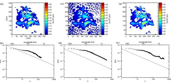
Figure 1a shows a sub-section of the COSMO-EU input data. Shown is a horizontal

25

(9)

ACPD

10, 21931–21988, 2010

L. Bugliaro et al.

Title Page

Tables Figures

◭ ◮

Back Close

Full Screen / Esc

Discussion

P

a

per

|

Dis

cussion

P

a

per

|

Discussion

P

a

per

|

Discussio

n

P

a

per

|

5/3 power law is expected at ranges between 10–30 km (k≈60–100) down to a few metres. In the original COSMO-EU data a 5/3 power law scaling seems to be present down to a wavelength range of 30 km.

Next a new Fourier spectrum is constructed from the large scale amplitudes (up to k=80) with small scale amplitudes (smaller than 30 km) obtained according to a 5/3

5

power law up to wavenumbers ofk=486 (according to a wavelength of 2×2.33 km). Using these new amplitudes (and related random phases) a new 2-D field of liquid water content for this layer is constructed by a backward Fourier transform on an in-creased horizontal resolution (Fig. 1c). As this new fields does not obey the original liquid water content on 7 km resolution each Fourier step is followed by a step restoring

10

this requisite. Figure 1e shows the resulting field of liquid water content after 3 iteration steps. The Fourier spectrum is not perfect (Fig. 1f) due to the requirement of conserv-ing the 7 km COSMO-EU-scale LWC distribution. This introduces discontinuities as the cloud gaps and also the block structure reflecting the original resolution. Nonethe-less, a field matching the COSMO-EU weather model cloud physics on COSMO-EU

15

resolution comprising statistically realistic small scale variability is generated.

Finally, atmospheric profiles from the COSMO-EU are extended to 120 km using the standard AFGL midlatitude summer atmosphere (Anderson et al., 1986). Trace gases not contained in the COSMO-EU output, in particular ozone, are also taken from this standard profile.

20

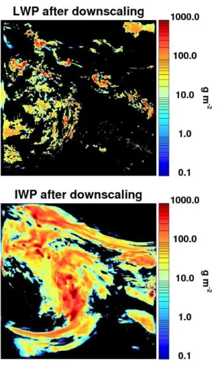
All final input fields have thus a resolution of 2.33 km and are given on a 972×972×50 grid. This way a scene of the size of Central Europe is generated with large structures of real weather related cloudiness and realistic detail on the small scales. In general such a resolution could as well be achieved by utilising the high-resolution COSMO-DE. However such a model run alone would not produce realistic variability on the

25

(10)

ACPD

10, 21931–21988, 2010

L. Bugliaro et al.

Title Page

Tables Figures

◭ ◮

Back Close

Full Screen / Esc

Discussion

P

a

per

|

Dis

cussion

P

a

per

|

Discussion

P

a

per

|

Discussio

n

P

a

per

|

3.1.3 Microphysics

Once resolution has been enhanced, cloud microphyics has to be associated to the cloud liquid and ice water fields. For water clouds liquid water content LWC [kg/m3] and e_ffective radiusreff=

R

r3n(r)dr/R

r2n(r)dr[µm] (n(r) is the particle size distribution in droplets/m3) are connected through

5

reff=

0.75·

LWC π·k·N·ρ

1/3

×10−6. (1)

Water droplet density N[1/m3] must be given (here = 150.0e6 1/m3) and is kept constant for all clouds in the domain. Thek factor describes the ratio between the vol-umetric radius of droplets, i.e. the mean volume radius,r_v=(Rn(r)r3dr/R

n(r)dr)1/3=

(R

n(r)r3dr/N)1/3and their effective radiusr_e_ff: k=r_v3/r_e3_ff and varies between 0.67±

10

0.07 for continental clouds and 0.8±0.07 for marine clouds according to Martin et al. (1994). Here we used a typical value ofk=0.75. ρis water density at 4◦C in kg/m3.

For ice clouds the parameterisation of randomly oriented hexagonal columns by (Wyser and Str ¨om, 1998; McFarquhar et al., 2003) is used which relates ice particle effective radiusreff[µm] to ice water content IWC [kg/m

3

] and temperatureT[K]:

15

b=−2.0+0.001·p273−T3·log((IWC/1000)/(50 g/m3))

r0=377.4+203.3·b+

37.91·b2+2.3696·b3 n_{f t}=(p3+4)/(3p3) r1=r0/nf t

20

(11)

ACPD

10, 21931–21988, 2010

L. Bugliaro et al.

Title Page

Tables Figures

◭ ◮

Back Close

Full Screen / Esc

Discussion

P

a

per

|

Dis

cussion

P

a

per

|

Discussion

P

a

per

|

Discussio

n

P

a

per

|

3.2 Radiative transfer model

In order to simulate satellite images from forecast model fields, a radiative transfer forward model needs to be applied. We take advantage of the libRadtran package (http://www.libradtran.org) which has been jointly developed since more than 10 years by Bernhard Mayer (Deutsches Zentrum f ¨ur Luft- und Raumfahrt, DLR, and Ludwig

5

Maximilians University in Munich, LMU), Arve Kylling (formerly NILU, Norway), and recently Ulrich Hamann (DLR), Claudia Emde and Robert Buras (LMU). libRadtran (Mayer and Kylling, 2005) provides a flexible interface to address all kinds of questions, and to compute irradiances (fluxes), actinic fluxes, radiances (intensities) and heating rates. Different methods are implemented, to calculate at very high spectral resolution

10

(line-by-line), at intermediate resolution (suited to simulate satellite instruments) and for integrated solar and thermal irradiances and radiances. It has been validated in several model intercomparison campaigns, and by direct comparison with observations (e.g., Mayer et al., 1997; Van Weele et al., 2000; DeBacker et al., 2001). Particular attention has been laid on the detailed and most realistic representation of water and ice clouds

15

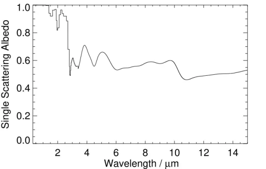
in the model. Optical properties of water droplets are computed using Mie theory and tabulated as a function of wavelength and effective radius. Ice crystals must not be assumed to be spherical particles and need therefore a special treatment since the conversion from microphysical to optical properties is much less defined. For this sim-ulation the parameterisation of Key et al. (2002) and Yang et al. (2000) for hexagonal

20

ice columns has been selected since it has an adequate spectral resolution. However, it only covers the solar spectral bands of MET-8/SEVIRI. Thus, starting from new single scattering optical properties provided by P. Yang (personal communication, 2006), we have developed a new parameterisation covering the complete solar and thermal spec-tral range between 0.25 and 100 µm, consistent with that of Key et al. (2002) and Yang

25

(12)

ACPD

10, 21931–21988, 2010

L. Bugliaro et al.

Title Page

Tables Figures

◭ ◮

Back Close

Full Screen / Esc

Discussion

P

a

per

|

Dis

cussion

P

a

per

|

Discussion

P

a

per

|

Discussio

n

P

a

per

|

rural aerosol model by Shettle (1989) in the boundary layer, background aerosol above 2 km, spring-summer conditions and a visibility of 50 km.

The selected one-dimensional radiative transfer solver is DISORT 2.0 by Stamnes et al. (1988, 2000), with 16 streams. Atmospheric gas absorption has been adopted from SBDART (Ricchiazzi et al., 1998) and relies on low resolution band models

devel-5

oped for the LOWTRAN 7 atmospheric transmission code (Pierluissi and Peng, 1985). It uses an exponential sum fit with a resolution of 20 cm−1. We adopted 15 spectral grid points to simulate each low resolution channel. The HRV channel was not simulated. 3.3 Surface

The underlying surface is described in terms of a Lambertian spectral albedo taken

10

from the MODIS albedo product MOD43C1 (Schaaf et al., 2002) for the year 2004 and the Julian day 225 for the area corresponding to the COSMO-EU region and the 7 solar MODIS channels contained in the spectral range 460 nm–2155 nm for which albedo has been derived. From MODIS thermal channels emissivity is derived by the MODIS land surface team and made publicly available in form of the MOD11C2 product (Wan

15

and Li, 1997). For the year 2004 and the Julian day 225 emissivities for wavelengths around 3.9, 8.7, 10.8 and 12.0 µm have been extracted from the appropriate product, transformed into albedos (emissivity₌1−albedo) and gathered into spectral albedo files for every resolution enhanced COSMO-EU pixel.

Albedo values are interpolated linearly between MODIS channels and assumed

con-20

stant below 460 nm and above 12.3 µm. For water bodies, surface albedo was com-puted in clear sky conditions for all MET-8/SEVIRI solar channels by using the ocean BRDF by Nakajima and Tanaka (1983) and Cox and Munk (1954a,b). These values were then again collected into a spectral albedo file and used as input to the radiative transfer simulations.

25

(13)

ACPD

10, 21931–21988, 2010

L. Bugliaro et al.

Title Page

Tables Figures

◭ ◮

Back Close

Full Screen / Esc

Discussion

P

a

per

|

Dis

cussion

P

a

per

|

Discussion

P

a

per

|

Discussio

n

P

a

per

|

3.4 Solar and viewing geometry

Solar zenith angles, satellite zenith angles and relative azimuth angles between sun and satellite have been produced for the geographic location of every COSMO-EU pixel in higher resolution, i.e. after downscaling. Sun zenith angle lies in the range 25.1◦–48.5◦(mean value=36.5◦), satellite zenith angle in the range 45.1◦–72.0◦(mean

5

value=58.6◦), relative azimuth angle in the range 0.0◦–12.2◦(mean value=4.5◦). The satellite selected is MET-8 (MSG-1) located at−3.4◦E, which was its operational orbit position until April 2008.

4 Simulations

Starting from the datasets and the radiative transfer model described in Sect. 3

radi-10

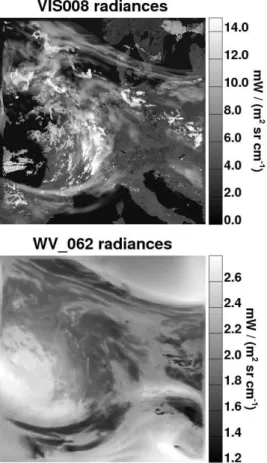
ances for every MET-8/SEVIRI channel have been computed. Two examples, the solar channel VIS008 and the thermal water vapour channel WV 062, are shown in Fig. 5.

To take into account the misleading definition of spectral radiance in the thermal range (eum, 2007) used by EUMETSAT’s Meteorological Product Extraction Facility for the processing of the Meteosat Second Generation data, an algorithm has been

15

written that transforms the correct spectral radiances (also called effective spectral radiances in the mentioned EUMETSAT document) produced by the radiative transfer model into spectral radiances (i.e. at a defined wavenumber) as they are expected by most algorithms for the detection of clouds that have been tuned and tested with real data so far.

20

After this correction radiances are convolved with the instrument point spread func-tion and brought into MET-8/SEVIRI projecfunc-tion by averaging all model values that be-long to a given satellite pixel.

The resulting MET-8/SEVIRI area simulated in this study thus comprises elements 1335 to 2111 and lines 3132 to 3536 in native coordinates (i.e. from the South-Eastern

25

(14)

ACPD

10, 21931–21988, 2010

L. Bugliaro et al.

Title Page

Tables Figures

◭ ◮

Back Close

Full Screen / Esc

Discussion

P

a

per

|

Dis

cussion

P

a

per

|

Discussion

P

a

per

|

Discussio

n

P

a

per

|

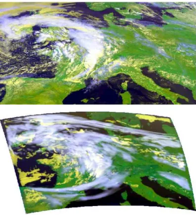
Based on these simulated channels a false colour composite has been produced and is plotted in Fig. 6 together with a false colour composite for the same time but from real MET-8 data. This way, the forecast of the COSMO-EU model can be directly evaluated. It shows that apart from a phase shift the cloud front is well described. However, it is also apparent that the model predicts too many cirrus clouds and to few

5

middle level clouds.

Plots of all channels are given in Appendix A, Figs. A1 and A2.

5 Cloud property retrievals

For this case study the APICS (Algorithm for the Physical Investigation of Clouds with SEVIRI) developed at DLR and the operational CMSAF software developed at the

10

French national meteorological service METEO FRANCE and the Royal Netherlands Meteorological Institute KNMI have been exemplarily selected to show the potential of this method to quantitatively validate cloud property retrievals. However, the focus does not lie on the validation of these particular retrieval algorithms but on the advantages and opportunities of the validation method. For this reason, the single algorithms are

15

only sketched in the following Sects. 5.1 and 5.2.

5.1 APICS

5.1.1 Cloud detection

The APICS cloud masking algorithm has inherited its structure from the EUMETSAT scenes detection algorithm (Lutz, 1999, 2002; Lutz et al., 2003). It is based on six

20

(15)

ACPD

10, 21931–21988, 2010

L. Bugliaro et al.

Title Page

Tables Figures

◭ ◮

Back Close

Full Screen / Esc

Discussion

P

a

per

|

Dis

cussion

P

a

per

|

Discussion

P

a

per

|

Discussio

n

P

a

per

|

and spatial coherence tests. The last test group aims at cirrus clouds alone: a cirrus cloud is detected when at least one of the cirrus tests described in Krebs et al. (2007) gives a positive result. This day and night cirrus algorithm consists of six sub-tests based on the infrared SEVIRI channels alone that exploit spectral as well as morpho-logical properties of cirrus clouds.

5

Threshold values used in the tests are either determined empirically, or derived from clear-sky albedo maps applying an atmospheric and viewing angle correction, or they are obtained from NWP (ECMWF) data by means of the libRadtran radiative transfer model (see also following Sect. 5.1.2).

5.1.2 Cloud top height

10

In order to infer cloud top height (i.e. pressure and temperature) two techniques are used: for opaque clouds, the measured IR 108 window channel brightness temper-ature is matched against a collocated atmospheric tempertemper-ature profile obtained from ECMWF analysis data. In the case of semi-transparent or sub-pixel clouds, however, this technique fails and the CO₂ slicing method is used where infrared channel

radi-15

ances at IR 108 and at IR 134 for black clouds located at different layers of the atmo-sphere are ratioed (Cayla and Tomassini, 1978; Szejwach, 1982; Nieman et al., 1993; Menzel et al., 1983; Schmetz et al., 1993). For both methods atmospheric profiles of temperature, pressure, water vapour and ozone are taken from ECMWF analyses with a 0.25◦×0.25◦ spatial resolution in longitude and latitude. Then, they are input to

li-20

bRadtran to simulate TOA radiances from black clouds located at different levels in the atmosphere. The vertical grid chosen here sets black cloud tops from the surface to 15 km altitude in 1 km steps.

5.1.3 Cloud top phase

Ice clouds are observed when the cirrus detection results by Krebs et al. (2007) are

25

(16)

ACPD

10, 21931–21988, 2010

L. Bugliaro et al.

Title Page

Tables Figures

◭ ◮

Back Close

Full Screen / Esc

Discussion

P

a

per

|

Dis

cussion

P

a

per

|

Discussion

P

a

per

|

Discussio

n

P

a

per

|

5.1.4 Cloud optical thickness and effective radius

Two channels are used for the determination of cloud optical thickness and cloud ef-fective radius: VIS006 (without water or ice absorption, respectively) and IR 016 (with water or ice absorption). The algorithm is based on the method described by Nakajima and King (1990) and Nakajima and Nakajima (1995), but has been adapted to

MET-5

8/SEVIRI in order to make use of the two solar channels instead of the three classical channels. Comparison of pre-calculated values of the reflectivities with corresponding measured quantities yields the optical thickness and effective radius that best repro-duce the measurements. For this purpose, reflectivities are tabulated in advance with libRadtran as a function of the relevant parameters (sun zenith angle, sensor zenith

10

angle, relative azimuth angle, surface albedo, cloud optical thickness, and effective particle radius). Water cloud effective radii run from 5 to 25 µm while ice cloud effective radii are in the range 6–84 µm. Water cloud optical properties are computed accord-ing to Mie theory, while ice cloud optical properties are parameterised after Key et al. (2002); Yang et al. (2000). In particular,refffor ice particles equals 34V/A, whereV is the

15

total volume of the particles andAis the total projected area. Information about surface albedo over land is extracted from the MODIS white albedo product MCD43C3 with a 0.05◦ spatial resolution for MODIS bands 1 (620–670 nm) and 6 (1628–1652 nm).

5.2 CMSAF

As a second test retrieval we selected the operational software used by the Climate

20

Monitoring Science Application Facility (CMSAF) for the creation of long term data sets of cloud properties. It consists of two parts: the first one includes the SAFNWC/MSG version1.4 (2008) software developed by METEO FRANCE (Derrien and LeGleau, 2005; SAFNWC, 2007) in the framework of the Science Application Facility for Now-casting (SAFNWC): in this study we used the products PGE01 (cloud mask) and

25

(17)

ACPD

10, 21931–21988, 2010

L. Bugliaro et al.

Title Page

Tables Figures

◭ ◮

Back Close

Full Screen / Esc

Discussion

P

a

per

|

Dis

cussion

P

a

per

|

Discussion

P

a

per

|

Discussio

n

P

a

per

|

5.2.1 Cloud detection

The algorithm is based on multispectral threshold techniques applied to each pixel and works in four steps. In the first step, a series of tests allows the identification of pixels contaminated by clouds or snow/ice. Similarly to APICS, reflectance tests, tempera-ture tests, temperatempera-ture difference tests, and spatial coherence tests are applied. Most

5

thresholds are determined from sun- and satellite-dependent look-up tables and make use of NWP forecast fields (surface temperature and total atmospheric water vapour content) and ancillary data (elevation and climatological data) from the GME model (Majewski, 1998; Majewski et al., 2002) with a resolution of 0.5◦×0.5◦ in latitude and longitude. These thresholds are computed at a spatial resolution of 16×16 pixels. The

10

second step allows on one side to reclassify pixels having a class type different from their neighbours. On the other side, an opacity and a complete overcast cloud flag is extracted for all cloud contaminated pixels. The third step consists in the assess-ment of the quality of the cloud detection process, while the last step identifies dust clouds and volcanic ash clouds and is applied to all pixels. More details can be found

15

in (SAFNWC, 2007).

5.2.2 Cloud top height

The basis for cloud top height retrievals are simulated vertical profiles of cloud free and overcast radiances and brightness temperatures for the thermal SEVIRI channels WV 062, WV 073, IR 134, IR 108 and IR 120. They are computed with the

RTTOV-20

7 radiative transfer model (Saunders et al., 2002) applied to NWP temperature and humidity vertical profiles with a horizontal spatial resolution of 32×32 SEVIRI pixels. For opaque clouds, the cloud top pressure corresponds to the best fit between the simulated and the measured IR 108 brightness temperatures. In the case of semi-transparent or sub-pixel clouds two bi-spectral techniques are used instead: first, the

25

(18)

ACPD

10, 21931–21988, 2010

L. Bugliaro et al.

Title Page

Tables Figures

◭ ◮

Back Close

Full Screen / Esc

Discussion

P

a

per

|

Dis

cussion

P

a

per

|

Discussion

P

a

per

|

Discussio

n

P

a

per

|

water vapour radiances vary linearly against IR window radiances as a function of cloud amount to extrapolate the correct cloud height (see references in Sect. 5.1.2). The final retrieved cloud top pressure is the averaged cloud top pressure obtained using single sounding channels. If this first step fails, the radiance ratioing method, adapted from the CO₂slicing by (Smith et al., 1970; Chahine, 1974; Smith et al., 1974; Smith and Platt,

5

1978; Menzel et al., 1983; Eyre and Menzel, 1989; Nieman et al., 1993), is applied successively to the window IR 108 and the sounding channels WV 073, WV 062 and IR 134 until a result is obtained. In case this result is warmer than the corresponding IR 108 brightness temperature, the method for opaque clouds is used instead.

5.2.3 Cloud top phase, cloud optical thickness and cloud e_ffective radius

10

The method iteratively interprets reflected solar radiation in the VIS006 and IR 016 channels in terms of cloud top phase, cloud optical thickness and cloud e_ffective radius. The physical basis for the determination of optical thickness and effective radius is the same as in Nakajima and King (1990) and Nakajima and Nakajima (1995): they are obtained by simultaneously comparing satellite observed reflectances at visible and

15

near-infrared wavelengths to look-up tables of simulated reflectances. In addition the method exploits the fact that at 1.6 µm the imaginary index of refraction is higher for ice particles than for liquid particles to infer cloud phase (see for instance Baum et al. (2000)).

The algorithm, described in Roebeling et al. (2006), starts with retrieving a cloud

20

optical thickness at 0.6 µm that is used to update the retrieval of particle size at 1.6 µm. This iteration process initially assumes ice clouds and continues until the retrieved cloud physical properties converge to stable values. In this case, infrared cloud emis-sivity is computed from the optical thickness according to (Minnis et al., 1993), and this quantitity is used to correct the 10.8 µm brightness temperature and obtain cloud

25

(19)

ACPD

10, 21931–21988, 2010

L. Bugliaro et al.

Title Page

Tables Figures

◭ ◮

Back Close

Full Screen / Esc

Discussion

P

a

per

|

Dis

cussion

P

a

per

|

Discussion

P

a

per

|

Discussio

n

P

a

per

|

climatological values of 8 µm for water and 26 µm for ice clouds, values close to those used by (Rossow and Schi_ffer, 1999). To obtain a smooth transition between assumed and retrieved effective radii a weighting function is applied to the effective radii of cloudy pixels with optical thickness between zero and eight.

The Doubling-Adding KNMI (DAK) monochromatic radiative transfer model (de Haan

5

et al., 1987; Stammes, 2001) is used to compile the required look-up tables. To trans-late line reflectances into SEVIRI channel reflectances, line-to-band conversion coef-ficients are computed by convolving Scanning Imaging Absorption Spectrometer for Atmospheric Chartography (SCIAMACHY, aboard the european research satellite EN-VISAT, Stammes et al., 2005) spectra with the SEVIRI spectral response functions

10

(Roebeling et al., 2006). For water clouds optical properties are obtained from Mie the-ory for effective radii (Hansen and Travis, 1974) between 1 and 24 µm; for ice clouds a homogeneous distribution of Cb, C1, C2 and C3 type imperfect hexagonal ice crys-tals from (Hess et al., 1998) is used with volumetric radii rv of 6, 12, 26 and 51 µm respectively (see Sect. 3.1.3 for the definition of this radii).

15

Cloud top phase corresponds to the resulting phase used in the τ–reff retrieval

(Wolters et al., 2008).

Unlike in the operational chain at CMSAF, the algorithm is run here without re-calibrating the solar channels to take into account the fact that simulated radiances are exact.

20

5.2.4 Cloud water path

Cloud water path CWP is derived from retrieved cloud optical thicknessτ and droplet effective radiusreff(see Sect. 5.2.3) by means of the relation (Stephens, 1978):

CWP=2

3τ reffρl, (2)

whereρ_l is the density of liquid water. Equality holds true when the size parameter

25

(20)

ACPD

10, 21931–21988, 2010

L. Bugliaro et al.

Title Page

Tables Figures

◭ ◮

Back Close

Full Screen / Esc

Discussion

P

a

per

|

Dis

cussion

P

a

per

|

Discussion

P

a

per

|

Discussio

n

P

a

per

|

of 2. This is only completely correct for water clouds and under the assumption that the cloud has a constant e_ffective radius vertical profile. The CPP algorithms first computes optical thicknessτand effective radiusreffand then derives cloud water path according

to the above equation. Although in the CMSAF processing chain only optical thickness and cloud water path are output, in this case e_ffective radius was added to the output

5

list.

6 Validation

Validation of cloud properties derived from satellite data is a complicated issue. Com-monly, either surface and airborne measurements are used, or intercomparisons of space-borne retrievals are performed in order to identify their strengths and

weak-10

nesses. However, only few in-situ data are available for the validation of quantities like cloud phase or particle size, or the combination of numerous instruments is re-quired. The major challenge consists in the different scales and different samplings of these measurements such that inherent discrepancies may exist that prevent the assessment of the performance or uncertainty of the satellite retrieval (e.g. Schutgens

15

and Roebeling, 2009). Thus, cloud properties retrieved from space-borne algorithms can only be partially validated at distinct points in space (and time) by means of sur-face or airborne measurements. In addition, three dimensional radiative effects and cloud inhomogeneity have been shown to introduce bias and considerable noise into the retrieved optical thickness and e_ffective radius (Zinner and Mayer, 2006). Noise

20

in particular precludes the use of in-situ observations when no statistically significant result can be achieved due to the usually limited availability of such data sets or to the rarity of satellite overpasses over the validation sites.

When comparing satellite retrievals with each other interesting aspects can be iden-tified and some light can be shed on the “true” cloud properties by considering the

25

(21)

ACPD

10, 21931–21988, 2010

L. Bugliaro et al.

Title Page

Tables Figures

◭ ◮

Back Close

Full Screen / Esc

Discussion

P

a

per

|

Dis

cussion

P

a

per

|

Discussion

P

a

per

|

Discussio

n

P

a

per

|

Here we show a paradigmatic validation of the two space-borne cloud retrievals APICS and CMSAF by means of the satellite scene simulated for MET-8/SEVIRI as explained in Sects. 4 and 5. This enables an objective validation of the algorithms since all the components of the Earth-atmosphere system that lead to the “observed” satellite radiances are known and can be directly compared to the output fields of the

5

retrieval algorithms.

In the following we will denote by “retrieved” all the cloud properties that are output of the satellite retrievals. In contrast, the word “real” or “reality” will be used to char-acterise those cloud properties that stem from the COSMO-EU weather model, have been subsequently downscaled and finally used as input to the radiative transfer model

10

for the simulation of the satellite scene. In fact, these are the cloud properties that lead to the radiance fields used in this study.

To make a comparison of retrieved and real cloud properties possible, real cloud properties have been projected to MET-8/SEVIRI grid in a similar way as the simulated radiances (see Sect. 4). More details will be given in the next subsections when cloud

15

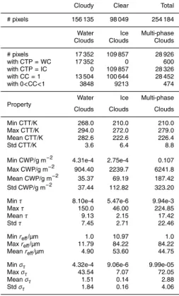
mask (Sect. 6.1), cloud top temperature (Sect. 6.3), cloud top phase (Sect. 6.2), cloud optical thickness (Sect. 6.4), cloud water path (Sect. 6.6) and cloud effective particle radius (Sect. 6.5: here a statistics over all cloud boxes inside a given MET-8/SEVIRI pixel is reported) will be addressed. However, Table 2 summarises all relevant real cloud properties of concern.

20

6.1 Cloud detection

Reality is represented in this case by the projection of the real binary (0/1) cloud mask originally defined on the downscaled COSMO-EU grid onto the MET-8/SEVIRI grid. This first yields a cloud cover mask from which a cloud mask has been obtained: all MET-8/SEVIRI pixels with cloud cover larger than zero have been defined to be cloudy.

25

(22)

ACPD

10, 21931–21988, 2010

L. Bugliaro et al.

Title Page

Tables Figures

◭ ◮

Back Close

Full Screen / Esc

Discussion

P

a

per

|

Dis

cussion

P

a

per

|

Discussion

P

a

per

|

Discussio

n

P

a

per

|

Second, the corresponding CMSAF dust and volcanic ash detection products were considered in order to cleanse the cloud mask from these spurious contaminations (which in this case were almost nonexistent). Finally, the CMSAF cloud mask quality flag was used to select only high confidence pixels. This provides us with two retrieved cloud masks that can be validated against the real cloud mask.

5

The discrepancies between APICS and real cloud mask as well as between CMSAF and real cloud mask are plotted in Fig. 7a and b. It can be immediately noticed that the two retrieved cloud masks are similar to each other. In fact, both cloud detection schemes prove their capability to reproduce the input cloud distribution. Anyway, diff er-ences between the two algorithms are present and missing knowledge about the real

10

cloud distribution in the observed domain could lead to erroneous conclusions. For instance, one can see in the South-Western part of the picture that no retrieval is able to detect the edges of the cloud field (the coincident red colour in the cloud mask dif-ference plots). On the contrary, some pixels are retrieved as overcast by both retrievals while in reality they are not (the turquoise colour).

15

In order to quantitatively assess the performance of the cloud detection algorithms, we evaluate various quantity including the Hanssen-Kuiper (HK) skill score (Hanssen and Kuipers, 1965), also called true skill score, applied to the pixels of the simulated scene. This measure is often used to evaluate the skill of precipitation forecasts (see Tartaglione (2010) and references therein) but also of cloud detection schemes (Reuter

20

et al., 2009). The HK skill score is based on the 2×2 contingency table of the detection events (Table 3). The four elements of the table are the hit a, false alarm b, miss c, and correct negative events d. The HK score, defined as

HK= ad−bc

(a+b)(c+d)= d c+d+

a

a+b−1, (3)

is independent of the distribution of events (really cloudy pixels) and nonevents (really

25

(23)

ACPD

10, 21931–21988, 2010

L. Bugliaro et al.

Title Page

Tables Figures

◭ ◮

Back Close

Full Screen / Esc

Discussion

P

a

per

|

Dis

cussion

P

a

per

|

Discussion

P

a

per

|

Discussio

n

P

a

per

|

that −1≤HK≤1. An HK score equal to 1 is associated with a perfect cloud detec-tion (b=c=0), while a score of −1 means that hits and correct negatives are zero (a=d=0). The HK score is equal to 0 for a constant forecast (either a=c=0 or b=d=0).

Considering first APICS (Fig. 7a), four features are observable: 1) an extended cloud

5

field is detected in the North-Eastern corner of the simulation which is actually much smaller; 2) some coastlines are classified as clouds; 3) many of the cloud border pixels, with fractional cloud cover, are not detected; 4) some mistakenly detected cloud over the Alps. In more detail, the domain considered contains 254 184 pixels, 156 135 are cloudy and the remaining 98 049 are clear. The retrieval output and the real cloud

10

mask both contain a cloud in 144 830 pixels, i.e. 93% of all cloudy pixels have been detected. Only≈7% of the cloudy pixels have not been detected (11 305 pixels), while the false alarm rate (clear pixels that are retrieved as cloudy) amounts to 8%, i.e. 19 105. Unfortunately, due to the features identified above, only approximately 81% of the input clear pixels are classified accordingly by APICS. Altogether, the retrieval

15

agrees with the reality, both clear or both cloudy, on approximately 88% of all pixels (223 774 pixels).The HK score amounts to 0.73.

Considering CMSAF, (Fig. 7b), as for APICS, some of the cloud border pixels with fractional cloud cover are not classified correctly, while in the Eastern part of the simu-lation some nonexistent cloud is detected. CMSAF detects 96% (149 843 pixels) of all

20

cloudy pixels, the false alarm rate amounts to 9.5% (24 197 pixels have been mistak-enly classified as cloudy). Altogether, only approximately 75% of the really clear pixels are classified as that by CMSAF (73 852 pixels). Retrieval and reality agree (both clear or both cloudy) on 88% of all pixels (223 695 pixels). The corresponding HK score is 0.71.

25

6.2 Cloud top phase

(24)

val-ACPD

10, 21931–21988, 2010

L. Bugliaro et al.

Title Page

Tables Figures

◭ ◮

Back Close

Full Screen / Esc

Discussion

P

a

per

|

Dis

cussion

P

a

per

|

Discussion

P

a

per

|

Discussio

n

P

a

per

|

ues for all pixels belonging to the same satellite pixel. Since more cloud phases could be present in every MET-8/SEVIRI pixel after re-projection, we decided to label every pixel according to the cloud top phase that appears most frequently in that pixel.

Since retrieved and real cloud mask differ, the validation of all retrieved cloud prod-ucts over every single retrieval algorithm is restricted to the pixels that are cloudy in

5

the real as well as in the retrieved cloud mask. This new cloud mask is called common cloud mask. Since two retrieval algorithms are investigated there are two common cloud masks, one for APICS and one for CMSAF.

The common cloud mask for APICS contains 144 830 cloudy pixels. Out of them, 14 516 are real water and 130 314 real ice clouds. The APICS retrieval classifies 59%

10

(8630 pixels) of the real water clouds as water and 99% (128 672 pixels) of the real ice clouds as ice. The large difference for water clouds (see Fig. 7a and c) is produced by the erroneous classification of the cloud field in the North-Eastern corner. Here, APICS evidently detects an extended cirrus cloud on top of the real water cloud and therefore assigns the wrong cloud top phase to these pixels. Since this cloud makes up more or

15

less half of all real water clouds, the retrieval performance is heavily affected. Overall, reality and APICS agree for almost 95% (137 302 pixels) of all common cloud pixels.

The common cloud mask for CMSAF is composed of 145 915 cloudy pixels. Out of them, 17 620 are real water and 128 295 real ice clouds. The CMSAF retrieval classifies almost 100% (17 604 pixels) of the real water clouds as water and 76% (97 441 pixels)

20

of the real ice clouds as ice . The large difference for ice clouds (see Fig. 7b and d) is produced by the erroneous classification of the cloud edges. Overall, reality and CMSAF algorithm agree for 79% (115 045 pixels) of all common cloud pixels.

6.3 Cloud top temperature

Cloud top temperature has a direct impact on the outgoing longwave radiation at

top-25

(25)

ACPD

10, 21931–21988, 2010

L. Bugliaro et al.

Title Page

Tables Figures

◭ ◮

Back Close

Full Screen / Esc

Discussion

P

a

per

|

Dis

cussion

P

a

per

|

Discussion

P

a

per

|

Discussio

n

P

a

per

|

and cloud top pressure, are neglected and the focus is put on cloud top temperatures. Again, the comparison between reality and retrievals is made on the basis of the com-mon cloud masks, regardless of the fact that some cloud pixels have been assigned the wrong thermodynamic phase since this information does not enter the computation of cloud top temperatures. Figure 7e and f show relative di_fferences between retrieved

5

and real cloud top temperatures for APICS and CMSAF respectively. Largest discrep-ancies are produced by APICS at the edges of cirrus clouds, but the overall agreement is good. The APICS mean di_fference is 3.1 K with a standard deviation of 10.6 K. This translates into a mean relative difference of 0.01 and standard deviation of 0.05 (the mean cloud top temperature of the real clouds investigated here is 228.8 K). This slight

10

overestimation of cloud top temperature means that cloud tops are located lower in the atmosphere by the APICS retrieval than they are in reality. This is a usual feature of the technique employed (see Sect. 5.1.2) since it determines the height (temperature) of the “radiative centre” of the cloud (Menzel et al., 1992), which is located further down in the atmosphere.

15

Figure 7f shows relative differences between CMSAF and real cloud top tempera-tures. The box structures that can be observed stem from the coarser resolution of the NWP model used for the preparation of the ancillary data set of black cloud radiances (see Sect. 5.2.3). Largest discrepancies (underestimations) are produced here at the edges of cirrus clouds but also some water cloud temperature is underestimated. The

20

overall agreement is good. The mean CMSAF difference is −16.4 K with a standard deviation of 37.3 K corresponding to a mean relative difference of−0.07 and standard deviation of 0.15. (The mean cloud top temperature of the real clouds investigated here is 229.9 K.) This underestimation of CMSAF cloud top temperatures is mainly produced at cloud edges. Only here, CMSAF cloud top temperatures are significantly lower than

25

(26)

ACPD

10, 21931–21988, 2010

L. Bugliaro et al.

Title Page

Tables Figures

◭ ◮

Back Close

Full Screen / Esc

Discussion

P

a

per

|

Dis

cussion

P

a

per

|

Discussion

P

a

per

|

Discussio

n

P

a

per

|

6.4 Cloud optical thickness

We restrict the validation to those pixels that belong to the common cloud masks, like in the previous sections (Sects. 6.2 and 6.3). Furthermore, we only consider a subset of this common cloud mask where both retrieved and real clouds have the same top thermodynamic phase and further distinguish between those cloudy pixels that

exclu-5

sively contain either water or ice clouds on one side and those that contain water and ice clouds at the same time. In this last pixel class called multi-phase in the following various cloud situations are collected: vertically extended clouds like cumulonimbus that are made up of liquid water droplets at their base and of ice crystals at their top belong to this class as well as pixels where a water cloud and a contiguous cirrus cloud

10

coexist as well as clouds containing mixed phase layers with both liquid water droplets and ice particles or cirrus clouds on top of liquid water clouds. This kind of clouds is outlined since it does not correspond to any of the cloud classes considered (pure water or pure ice) in the retrieval cloud optical thickness and effective radius such that larger inaccuracies are expected. The distribution of real water, ice and multi-phase

15

clouds is shown in Fig. 8.

This leaves us with 8548 water cloud, 100 480 ice cloud and 27 444 multi-phase cloud pixels for APICS and 16 829 water cloud, 75 768 ice cloud and 22 224 multi-phase cloud pixels for CMSAF. Notice that these numbers are di_fferent from those exposed in Sect. 6.2 since we consider three classes here instead of two (see also

20

Table 2).

Evidently, both retrievals are capable of reproducing the real distribution of cloud optical thicknesses as can be seen from Fig. 9 which depicts histograms and scatter plots of retrieved and real optical thickness.

As far as APICS is concerned, the distribution of water and ice clouds is better

ap-25

(27)

ACPD

10, 21931–21988, 2010

L. Bugliaro et al.

Title Page

Tables Figures

◭ ◮

Back Close

Full Screen / Esc

Discussion

P

a

per

|

Dis

cussion

P

a

per

|

Discussion

P

a

per

|

Discussio

n

P

a

per

|

In fact, the histogram peak around optical thickness 10 for multi-phase clouds is more pronounced in the retrieval than in reality. For water clouds, APICS misses the first peak while it overestimates the second one. Plots d–f in Fig. 9 confirm a good corre-lation between real and retrieved water and ice cloud optical thicknesses respectively (0.977 and 0.996). Here of course both retrieved and model results are for pixels of

5

the common cloud mask. Altogether, APICS slightly underestimates real optical thick-ness: mean differences between retrieved and real cloud optical thickness amount to

−0.71 for water and −0.13 for ice clouds, with a standard deviation of 1.20 for water clouds which is higher than for ice clouds (0.40). Multi-phase clouds show a worse correlation of 0.957, a mean underestimation of−6.50 and a larger scattering of 8.72.

10

However, those multi-phase clouds that were treated as water clouds by APICS lie on the one-one line.

Finally, relative differences (Fig. 10) between optical thicknesses of real and retrieved water and ice clouds are both quite sharply peaked around−0.04 while the relative dif-ference distribution of multi-phase clouds is much more flat with a peak around−0.45.

15

Considering now CMSAF results (blue lines in Fig. 9a–c), a slightly different be-haviour can be observed. While the histogram curves of retrieved and real cloud op-tical thickness occurrences overlap for multi-phase clouds (Fig. 9c), the water cloud distribution does not account for two peaks (Fig. 9a): real water clouds have two peaks at around optical thickness 1–2 and 7–8 while retrieved optical thicknesses are peaked

20

in between at 2–3. For ice clouds (Fig. 9b), CMSAF underestimates the occurrence of thin clouds (τ≤2) and overestimates the optical thickness of the remaining clouds (τ >2). Scatter plots (Fig. 9g–i) show a good one-to-one correlation for water clouds with a slight tendency to underestimation, apart from some data point whose optical thickness is overestimated by CMSAF by a factor of 2 to 5 (Fig. 9d). The effect of these

25

(28)

ACPD

10, 21931–21988, 2010

L. Bugliaro et al.

Title Page

Tables Figures

◭ ◮

Back Close

Full Screen / Esc

Discussion

P

a

per

|

Dis

cussion

P

a

per

|

Discussion

P

a

per

|

Discussio

n

P

a

per

|

trend towards overestimation and a correlation coefficient of 0.774. The scatter plot of CMSAF against real ice optical thicknesses in Fig. 9e also shows a structure that may be related to the four ice cloud models used in the compilation of the look-up tables for the retrieval (see Sect. 5.2.3). The mean difference of ice cloud optical thickness between CMSAF and reality amounts to 2.36 with a standard deviation of 5.0, mean

5

relative difference is 0.80 with a similar relative standard deviation of 0.78. Multi-phase clouds (Fig. 9f) show a relatively good agreement with a tendency to overestimation as well as a large scattering (correlation coe_fficient₌0.79, mean di_fference₌9.40, stan-dard deviation=36.9, mean relative difference=0.34, mean standard deviation=0.92). In particular, when the multi-phase cloud was classified as a water cloud by CMSAF, a

10

reasonable agreement was found.

The distribution of relative differences between optical thicknesses of real and re-trieved clouds is shown in Fig. 10 for CMSAF as well. Water clouds show a peak at around 0.05 while ice and multi-phase clouds present more uniform distributions that confirm the tendency to overestimation already observed in Fig. 9 and in particular the

15

large scattering mentioned above.

Considering the different accuracies of the two (ice cloud) retrievals it must be em-phasised that ice cloud properties show a relevant dependence on ice particle shape and the parameterisation of their optical properties. While APICS uses optical proper-ties for hexagonal columns by (Key et al., 2002; Yang et al., 2000), CMSAF considers

20

imperfect hexagonal crystals according to (Hess et al., 1998). In our reality, also (Key et al., 2002; Yang et al., 2000) was used such that APICS had a clear advantage in this case.

6.5 Cloud effective radius

Effective radius is a quantity that is particularly difficult to validate for various reasons.

25

(29)

ACPD

10, 21931–21988, 2010

L. Bugliaro et al.

Title Page

Tables Figures

◭ ◮

Back Close

Full Screen / Esc

Discussion

P

a

per

|

Dis

cussion

P

a

per

|

Discussion

P

a

per

|

Discussio

n

P

a

per

|

in the 1.6 µm MET-8/SEVIRI channel where water droplets not only reflect but also ab-sorb solar radiation. This absorption increases with cloud droplet size: the greater the droplet absorption the less the cloud reflectance. However, these reflectances may also depend on optical thickness such that the value of the effective radius must always be determined at the same time as optical thickness which on its turn largely depends on

5

the 0.6 µm MET-8/SEVIRI channel where absorption is marginal. However, real-world clouds are usually vertically inhomogeneous and a retrieval gives optical thickness and effective radius of a homogeneous cloud having (nearly) the same spectral reflectances as the measured one. Thus, effective radius does not only depend on the absorbing intensity of the channel used (Platnick, 2000) but is also highly retrieval dependent and

10

there is no real truth to compare with. Nevertheless, the compilation of e_ffective radius properties contained in Table 2 can be used to argue about some aspects of the re-trieval results. The values reported there stem from a statistical evaluation of all real cloud boxes and give some information about the e_ffective radius distribution of the real cloud: minimum, maximum and mean values of encounteredreff values are listed for

15

water, ice and multi-phase clouds.

Furthermore, while the definition of e_ffective radius for spherical liquid water droplets after Hansen and Travis (1974) asreff=

R

r3n(r)dr/R

r2n(r)dr is commonly accepted (n(r) being the droplet size distribution), for ice clouds various definitions are possible (see McFarquhar and Heymsfield, 1998). APICS and CMSAF use two definitions that

20

can be mapped to each other (Schumann et al., 2010) such that a direct comparison between them is possible.

For these reasons we only show here the histograms of the two retrieval results and make some comments on their main features. Also in this case we consider the com-mon cloud mask between the two satellite retrieval results with the additional exclusion

25

of all the really clear pixels that have been mistakenly classified as cloudy by both algorithms (see Sect. 6.1).