ABSTRACT: To date, the quantitative genetics theory for genomic selection has focused mainly on the relationship between marker and additive variances assuming one marker and one quanti-tative trait locus (QTL). This study extends the quantiquanti-tative genetics theory to genomic selection in order to prove that prediction of breeding values based on thousands of single nucleotide poly-morphisms (SNPs) depends on linkage disequilibrium (LD) between markers and QTLs, assum-ing dominance. We also assessed the efficiency of genomic selection in relation to phenotypic selection, assuming mass selection in an open-pollinated population, all QTLs of lower effect, and reduced sample size, based on simulated data. We show that the average effect of a SNP substitution is proportional to LD measure and to average effect of a gene substitution for each QTL that is in LD with the marker. Weighted (by SNP frequencies) and unweighted breeding value predictors have the same accuracy. Efficiency of genomic selection in relation to phenotypic selection is inversely proportional to heritability. Accuracy of breeding value prediction is not affected by the dominance degree and the method of analysis, however, it is influenced by LD extent and magnitude of additive variance. The increase in the number of markers asymptotically improved accuracy of breeding value prediction. The decrease in the sample size from 500 to 200 did not reduce considerably accuracy of breeding value prediction.
Keywords:genome-wide selection, additive value prediction, prediction accuracy
1Federal University of Viçosa − Dept. of General Biology, Av.
Peter Henry Rolfs s/n − 36570-900 − Viçosa, MG − Brazil.
2University of Hohenheim/Institute of Crop Science −
Biostatistics Unit − 70599 − Stuttgart − Germany.
3Federal University of Viçosa − Dept. of Animal Science.
*Corresponding author <[email protected]>
Edited by: Antonio Augusto Franco Garcia
Quantitative genetics theory for genomic selection and efficiency of breeding value
José Marcelo Soriano Viana1*, Hans-Peter Piepho2, Fabyano Fonseca e Silva3
Received November 05, 2014 Accepted December 10, 2015
Introduction
Genomic selection is the process of identifying su-perior individuals based on breeding values predicted from the analysis of thousands of molecular marker loci and a limited number of phenotypic records (Meuwissen et al., 2001). Because the statistical analysis involves a very large number of markers and relatively few obser-vations, marker effects that comprise the genomic value cannot be simultaneously predicted by the least squares regression (Goddard and Hayes, 2007). Several regular-ized whole-genome regression and prediction methods are reviewed by Campos et al. (2013), who emphasized that Bayesian LASSO (least absolute shrinkage and selec-tion operator) performs well across traits and GBLUP (genome best linear unbiased prediction) performs well for most traits.
Relevant theoretical and applied studies have shown the efficiency of genomic selection (Daetwyler et al., 2013). Meuwissen et al. (2001) showed that Bayes-ian methods were the most accurate to predict breeding values and identified quantitative trait loci (QTLs) with higher effects. The decrease in the number of phenotypic values and in marker density reduced accuracy. Predic-tion accuracy in future generaPredic-tions decreased, neverthe-less, magnitude ensured efficient selection. Comparable results were obtained by Goddard (2009) and Grattapa-glia and Resende (2011). Jannink et al. (2010) considered that the paradigm of lower efficiency of marker-assisted selection in relation to phenotypic selection for quantita-tive traits can change with the establishment of genomic selection. Goddard (2009), however, observed higher
ef-ficiency of genomic selection in relation to phenotypic selection only for the short term. Grattapaglia and Re-sende (2011) stated that genomic selection in forestry breeding could be superior to pedigree-based BLUP se-lection when the cycle length for the first strategy was at least 75 % less than the cycle length by pedigree-based BLUP selection.
Until now, the quantitative genetics theory for ge-nomic selection has focused mainly on the relationship between marker and additive variances assuming one marker and one quantitative trait locus (QTL). This study extends the quantitative genetics theory for genomic se-lection to prove that prediction of breeding value based on thousands of single nucleotide polymorphisms (SNPs) depends on linkage disequilibrium (LD) between mark-ers and QTLs, assuming dominance. We also assessed efficiency of genomic selection toward phenotypic selec-tion, assuming mass selection in an open-pollinated pop-ulation, all QTLs of lower effect, and reduced sample size, based on simulated data.
Materials and Methods
Theory
Expressing a marker effect, the variance of a mark-er effect and the predictor of a genetic value (genomic value) as a function of marker allelic frequencies, QTL effects and frequencies and LD values between QTLs and markers, assuming s markers and k QTLs, is an un-wieldy task. However, general functions could be derived assuming one marker and one QTL, one marker and two QTLs, and two markers and one QTL. These expressions
are useful to derive and assess predictors of breeding value, identify parameters predicted by a whole-genome analysis and their interpretation and compute maximum accuracy of breeding value prediction with genotyping and phenotyping in the same individual.
Relationship between marker and QTL additive and dominance effects
Assume a Hardy-Weinberg equilibrium population (generation −1). Further, assume that B and b are alleles of a QTL and that C and c are alleles of a SNP (single nucleotide polymorphism) locus. B and b are alleles that increase and decrease the trait expression, respectively. Assuming linkage, probabilities of gametes BC, Bc, bC, and bc in the gametic pool of the population are, respec-tively,
PBC p pb c bc
(−1)= + ∆(−1)
PBc p qb c bc
(−1)= −∆(−1)
PbC q pb c bc
(−1)= − ∆(−1)
Pbc q qb c bc
(−1)= + ∆(−1)
where p is the frequency of the major allele (B or C), q = 1 – p is the frequency of the minor allele (b or c), and ∆bc− =PBC− Pbc− −PBc− PbC−
(1) (1) (1) (1) (1)
is the measure of LD (Kempthorne, 1957). The genotypic values of individuals BB, Bb, and bb are
GBB =M+2qb b+ −
(
2q db b)
=M+ABB+DBB2
α
GBb =M+
(
qb−pb)
αb+2p q db b b=M+ABb+DBbGbb=M+ −
(
2pb b)
+ −(
2p db b)
=M+Abb+Dbb2
α
where M is the population mean, ab=ab + (qb – pb)db is the average effect of a gene substitution, db is the domi-nance deviation (deviation between the genotypic value of heterozygotes and the mean of genotypic values of homozygotes (mb)), and A and D are QTL additive and dominance genetic values, respectively. Parameter ab is the deviation between the genotypic value of the homo-zygote of higher expression and mb.
Genotype probabilities in generation 0 are (for simplicity, superscript (0) – for generation 0 – was omit-ted in all parameters that depend on LD measure of gen-eration −1)
f22 p pb c p pb c bc bc
2 2 2 1 1 2
= + ∆(−)+ ∆ (−)
f21 p p qb c c p qb c pc bc bc
2 1 1 2
2 2 2
= +
(
−)
∆(−)− ∆(−)f20 p qb c p qb c bc bc
2 2 1 1 2
2
= − ∆(−)+ ∆ (−)
f12 p q pb b c qb p pb c bc bc
2 1 1 2
2 2 2
= +
(
−)
∆(−)− ∆(−)f11 f11g f11n p q p qb b c c qb pb qc pc bc bc
1 1
4 2 4
= + = +
(
−)
(
−)
∆(−)+ ∆(−) 2f10 p q qb b c qb p qb c bc bc
2 1 1 2
2 2 2
= −
(
−)
∆(−)− ∆(−)f02 q pb c q pb c bc bc
2 2 1 1 2
2
= − ∆(−)+ ∆ (−)
f01 q p qb c c q qb c pc bc bc
2 1 1 2
2 2 2
= −
(
−)
∆(−)− ∆(−)f00 q qb c q qb c bc bc
2 2 1 1 2
2
= + ∆(−)+ ∆ (−)
where fij is the probability of the individual with i and j copies of allele B of QTL and allele C of the SNP (i, j = 2, 1, or 0). Indices g and n identify double heterozygotes in coupling and repulsion phases.
The average genotypic values of individuals CC, Cc, and cc are
G
p f G f G f G
M q q
CC c
BBCC BbCC bbCC
c bc b c
=
(
+ +)
= + + −
1
2 2
2 22 12 02
2
κ α
(
κκbc b2d)
=M+2αC+DCC =M+ACC+DCCG
p q f G f G f G
M q p
Cc c c
BBCc BbCc bbCc
c c bc b
= ( + + )
= +( − ) +
1
2 21 11 01
κ α 22p q 2d M D M A D
c cκbc b= +(αC+αc)+ Cc= + Cc+ Cc
G
q f G f G f G
M p p
cc c
BBcc Bbcc bbcc
c bc b
=
(
+ +)
= + −
(
)
+ −1
2 2
2 20 10 00
κ α
(
cc2κbc b2d)
=M+2αc+Dcc=M+Acc+Dccwhereκbc bc
c c p q
=∆
−
(1)
,
aC = qcκbcabandac = –pcκbcab are the average effects of SNP alleles, and A and D are additive and dominance values in relation to the SNP locus. The average effect of substituting allele C for c is aSNP=aC – ac=κbcab. Domi-nance deviation for the SNP is dSNP= κbc bd
2 . SNP additive
effects (consequently, average effect of a SNP substitu-tion and SNP additive value) are proporsubstitu-tional to the LD value and the average effect of a QTL substitution. Fur-thermore, SNP dominance deviation (consequently, SNP dominance value) is proportional to squared LD value and QTL dominance deviation. The expectation of both SNP additive and dominance values equals zero. LD measure can also be expressed as ∆− = −
bc rbc p q p qb b c c
(1) (1) ,
where rbc
(−1)
is the correlation between values of alleles in both loci (one for B and C, and zero for b and c) in the ga-metic pool of generation −1 (Hill and Robertson, 1968).
Relationship between SNP additive value and QTL additive value
If there is LD between a SNP and a QTL, additive and dominance values in relation to the SNP are propor-tional to additive and dominance values regarding QTL, respectively. The SNP additive values are
ACC=
(
qc/qb)
κbcABB=2qc/(
qb−pb)
κbcABb= −(
qc/pb)
κbcAbbACc=
(
qc−pc)
qb bcABB=(
qc−pc)
(
qb−pb)
bcABb= −
/2 κ / κ
A p q A p q p A
p p A
cc c b bc BB c b b bc Bb
c b bc b
= −
(
)
= −(
−)
=(
)
/ / / κ κ κ 2 bbThus, a predictor of the QTL additive value is the SNP additive value, that is,AQTL ASNP SNP
1
1
= =µ α , where
m1=2qc for SNP genotype CC, m1=qc – pc for Cc, or m1=–
2pc for cc. This predictor has been used in most whole-genome analysis. However, in some analysis, predictor
AQTL2 SNP 2
= µ α has been used, where µ2 = 2 for SNP genotype
CC, µ2 = 1 for Cc, or µ2 = 0 for cc. It shows that E AQTL1
0
(
)
= ,E AQTL2 pc SNP 2
(
)
= α and Var AQTL 1(
)
=Var A(
QTL)
2=Cov A
(
A)
QTL,QTL1 =
(
)
Cov AQTL,AQTL
2 =2p q 2
c cαSNP = σA(SNP) 2
where σ A SNP( ) 2
is the SNP additive variance. Thus, both predictors have the same accuracy (correlation between the additive value for QTL and the value predicted by the SNP), given by
ρ ρ
σ
σ
A A A A
A
A
QTL QTL QTL QTL
SNP
QTL
, ,
( )
( )
1 2
2
2
= =
where σ2A(QTL) p qb bαb2
2
= is the QTL additive variance.
The SNP additive variance can be expressed as ∆
{
−}
bc p q p qb b c c A
( )
( )
/
1 2 σ2
QTL . The previous expression is a
gen-eralization of the results provided by Gianola et al. (2009) and Goddard (2009). However, assuming dominance, SNP variance is σA(SNP) σD(SNP)
2 + 2
, where σD(SNP) p q dc c SNP
2 2 2 2
4
=
is SNP dominance variance. SNP dominance vari-ance can be expressed as
{
∆− }
bc p qb b D
( )
( )
/
1 2σ2
QTL, where
σD(QTL) p q db b b
2 =4 2 2 2
is QTL dominance variance.
Parametric values of regression coefficients in a whole-genome analysis
Parametric values of regression coefficients in a whole-genome analysis are derived by a regression anal-ysis that relates the genotypic value (G) to the number of copies of one allele of each SNP. Assuming one SNP in LD with one QTL, the additive-dominance model is G = β0 + β1x + β2x2 + ε (x = 2, 1, or 0). The model can
be expressed as y (9 × 1) = X (9 × 3). β (3 × 1) + error vector (9 × 1), where y is the vector of QTL genotypic values, conditional to SNP genotype, X is the incidence matrix, and β is the parameter vector. Assuming a bial-lelic QTL, there are 3 × 3 = 9 genotypes for QTL and marker (for example, BBCc). Because the genotypes have different probabilities, we defined the matrix of geno-type probabilities as P (9 × 9) = diagonal{fij}. Thus, for the complete or reduced model, β = (X'PX)–1 (X'Py) and
R(.) = β'(X'Py), where R(.) is the reduction in the total sum of squares due to fitting the model. Finally, fitting three regression models – the complete model G = β0 +
β1x + β2x
2 + ε and reduced models G = β
0 + β1x + ε
(no dominance) and G = β0 + ε (no QTL in LD with the marker) – shows that
β0 =M (fitting model G = β0 + ε)
β1 =aSNP (fitting model G = β0 + β1x + ε)
β2 =–dSNP (fitting model G = β0 + β1x + β2x2 + ε)
R β β1 0 R β β0 1 R β0 σA
2
(
)
=(
,)
−( )
= (SNP)R β β β2 0 1 R β β β0 1 2 R β β0 1 σD
2
, , , , ( )
(
)
=(
)
−(
)
= SNPwhere R(..) is a difference between two nested R(.) terms with the additional effect stated before the vertical bar and the effect(s) common to both models after the bar.
Thus, the intercept of the model G = β0 + ε is the
population mean, the regression coefficient of the simple linear model (G = β0 + β1x + ε) is the average effect of substitution for the SNP locus, and coefficient β2 in the complete model is the negative of SNP dominance de-viation. The additive and dominance variances relative to SNP are the sum of squares of linear and quadratic effects. Thus, a whole-genome analysis provides average effects of SNP substitution and SNP dominance devia-tions.
The alternative model is G = β0 + β1x1 + β2x2 +
ε, where x1 = 1, 0, or −1 if the individual is CC, Cc, or cc, and x2 = 0 or 1 if the individual is homozygous or heterozygous, respectively. Using the same procedure, we observed that the only difference in relation to the previous model is that β2 = dSNP (fitting model G = β0 +
β1x1 + β2x2 + ε). Most studies on genomic selection have fitted this model in which SNP genotypic values are de-fined as GCC = mc + ac, GCc = mc + dc, and Gcc = mc – ac. SNP parameters are
mc = M + (qc – pc)aSNP – (1 –2pcqc)dSNP
ac = aSNP – (qc – pc)dSNP
dc = dSNP
Accuracy of breeding value prediction
To derive a general function for breeding value prediction accuracy, we further considered one QTL (B/b) and two SNPs (C/c and E/e) in LD and two QTLs and one SNP in LD. Regarding predictors of the additive value for QTL based on two SNPs, we have E AQTL
1
0
(
)
= ,E AQTL pc SNP(C) pe SNP(E)
2
2
(
)
= α +2 α ,Var AQTL 1(
)
=Var A(
QTL)
2=σ +σ + ∆− =
α α σ
A( ( ))C A( ( ))E ce C E A
( )
( ) ( ) ( )
SNP SNP SNP SNP SNP
2 2 4 1 2
, and Cov AQTL,AQTL1
(
)
=Cov A(
QTL,AQTL)
2 =σ +σ
A(SNP( )A) A(SNP( )C)
2 2 ,
where σ A(SNP)
2 is the variance of the additive value
dictor (additive genomic value variance). Thus, both pre-dictors have the same accuracy, given by
ρ ρ σ σ
σ σ
A A A A
A C A E
A
QTL QTL QTL QTL
SNP SNP
QTL
, ,
( ( )) ( ( ))
( )
1 2
2 2
2
= = +
A A(SNP) 2
The additive-dominance model is G=β0+β1 1x +β2 2x +β3 1x2+β x +ε
4 2
2 , where indices 1 and
β0 = M (fitting model G = β0 + ε)
β1 = κbcab = aSNP(C) (fitting model G = β0 + β1x1+ ε)
β2 = κbeab = aSNP(E) (fitting model G = β0 + β2x2+ ε)
β3 κ
2
= −dSNP( )C = − bc bd (fitting model G=β0+β1 1x +β3 1x +ε 2
)
β4 κ
2
= −dSNP( )E = − be bd (fitting model G=β0+β2 2x +β4 2x +ε 2
)
R β β1 0 p qc cα C σ C
2 2
2
(
)
= SNP( ) = A(SNP( ))R β β2 0 p qe eα E σ
2 2
2
(
)
= SNP( )= A(SNP(E))R β β3 0 β1 p q dc c C σD C
2 2 2 2
4
, ( ) ))
(
)
= SNP = (SNP(R β β4 0 β2 p q de e E σD
2 2 2 2
4
, ( ) ))
(
)
= SNP = (SNP(Ewhereκbc bc c c p q =∆ − (1)
and κbe be e e p q =∆ − (1)
Assuming now a SNP (C/c) in LD with two QTLs (B/b and E/e) and defining E and e as alleles for the sec-ond QTL, where E and e are the alleles that increase and decrease trait expression,
β0 = M
β1 = κbcab + κceae = aSNP
β2 κ κ
2 2
= −
(
bc bd + ce ed)
= −dSNPR β β1 0 p qc cα σA
2 2
2
(
)
= SNP= (SNP)R β β2 0β1 p q dc c σD
2 2 2 2
4 ,
(
)
= SNP = (SNP)whereκce ce c c p q =∆ − (1)
.
Thus, correlation between the additive value for QTLs and the value predicted by the SNP is
ρ ρ σ
σ
A A A A A
A
, ,
( )
( )
1 2
2
2
= = SNP
QTL
where σA( ) p qb bαb p qe eαe beα αb e
( ) QTL
2 2 2 1
2 2 4
= + + ∆−
(Viana, 2004).
Generalizing, the additive genetic value relative to k QTLs predicted by s SNPs is
A r r s r 1 1 1 = =
∑
µ α( ) SNP( ) or A r r s r 2 2 1 = =∑
µ α( ) SNP( ).Both predictors have the same accuracy, given by
ρA A ρA A σA r σ σ
r s
A A
,1 ,2 ( ( ))/ ( )
2
1
2 2
= =
=
∑
SNP SNPwhere σA(SNP( ))r p qr rαSNP( )r
2 =2 2
is the additive variance for SNP r,
αSNP( )r (ri) α κ α
r r i
k
i ri i i k p q = ∆ = − = ′ = ′
∑
1∑
1 1
is the SNP average effect of allele substitution (k' is the number of QTLs in LD with the SNP r),
σA i iα α α
i k
i ij i j
j k i k p q 2 1 2 1 2 1 1 2 4 = + ∆ = − = = < −
∑
∑
∑
( )(Viana, 2004) is the
ad-ditive variance, and
σA r rα α α
r s
r rt r
t s r p q ( ) ( )
SNP SNP( ) SNP( ) SNP(t)
2 1 2 1 2 1 2 4 = + ∆ = − = =
∑
∑
< < −∑
s1(Viana, 2004) is variance of the additive value predictor (additive genomic value variance).
Due to shrinkage, the sum of SNP variances has low magnitude and provides a very low estimate of breeding value accuracy. For population 1, generation 0, simula-tion 1, expansion volume, heritability of 0.7, sample size 500, and average SNP density of 0.1, the sum of the SNP variances is 0.037924 (covariance between the estimated breeding value and the true breeding value is 1.770058). A less biased estimator of the breeding value accuracy is σA(SNP)/σA
2 2 . For the described scenario, phenotypic
variance is 4.937459 and variance of predicted breeding values is 1.641861. Assuming a narrow sense heritability estimate of 0.6 (parametric value), accuracy is 0.7445. The correct estimate is 0.8068.
Simulation
The simulation program – REALbreeding (avail-able on request) – is under development by the first author, using the software REALbasic. Firstly, 5000 SNPs and 100 QTLs were randomly distributed across ten chromosomes (500 SNPs and 10 QTLs per chromo-some). The average distance between adjacent SNPs was 0.1 cM. QTLs were distributed in the regions covered by SNPs. Then, a Hardy-Weinberg equilibrium population with LD was generated - a composite of two populations (population 1). The composite was generated crossing two populations in linkage equilibrium followed by a generation of random crosses. Finally, the software com-puted all genetic parameters based on user input, which includes minimum and maximum genotypic values for homozygotes (Gmin and Gmax), degree of dominance (d/a), direction of dominance, and broad sense herita-bility. True additive and dominance genetic values and variances were computed from the population gene fre-quencies (random values), LD values (see parametric LD in a composite in the following subsection), average ef-fects of a gene substitution (a) and dominance deviations (d). Because Gmin = km – (nq.π + nm)a and Gmax = km
+ (nq.π + nm)a, where m is the average genotypic value of homozygotes, k is the number of genes, nq is the
num-ber of QTLs, and nm is the number of minor genes, we have m = (Gmin + Gmax)/2k, a = (Gmax – km)/(nq.π +
dominance deviations are random values. Phenotypic values are computed from the true population mean, additive and dominance values and from error effects sampled from a normal distribution. Error variance is computed from broad sense heritability.
We considered three popcorn traits, three SNP densities, two heritabilities, two sample sizes, and two related populations with LD, totaling 72 scenarios. For each scenario, 50 simulations were carried out. Mini-mum and maxiMini-mum genotypic values of homozygotes for grain yield, expansion volume and days to maturity were 20 and 200 g per plant, 5 and 50 mL g−1, and 100
and 160 days, respectively. Positive unidirectional domi-nance (0 < (d/a)i≤ 1.2) was assumed for grain yield. Bi-directional dominance (-1.2 ≤ (d/a)i ≤ 1.2) was assumed for expansion volume. Absence of dominance ((d/a)i = 0) was assumed for days to maturity. Other SNP den-sities, one marker every cM and one marker every 10 cM on average, were obtained by random choices of 51 and 6 SNPs per chromosome, respectively, also using the REALbreeding software. Broad sense heritabilities were 0.3 and 0.7. Thus, accuracies of phenotypic values were 0.548 and 0.837, respectively. The sample size was 500 or 200 individuals genotyped and phenotyped. The ef-fective population sizes were 1000 and 400.
Other four populations were simulated. To assess influence of the LD level on breeding value prediction accuracy, we recombined population 1 (generation 0) for five generations of random mating, assuming absence of selection and mutation, and keeping the sample size 500 (population 1, generation 5). Regarding SNPs, aver-ages of absolute LD values (difference between gametic frequencies observed and expected under linkage equi-librium) in LD blocks in population 1, generation 0, were 0.0978, 0.1073, and 0.1413 for densities 10, 1, and 0.1 cM, respectively. Values for population 1, generation 5, were 0.0581, 0.0565, and 0.0901, respectively. LD blocks were defined based on an LOD (logarithm [base 10] of odds) score 3 (to declare LD for two linked SNPs), also using the REALbreeding software. The corresponding r2 (square of
the correlation coefficient between alleles of two loci) val-ues were 0.1785, 0.2089, and 0.4079 for generation 0 and 0.0843, 0.0829, and 0.2420 for generation 5. We also sim-ulated a population with lower average LD and similar additive variance (population 2), relative to the population 1, generation 0. The average of absolute LD values in LD blocks in population 2, generation 0, were 0.0475, 0.0560, and 0.0557 for densities 10, 1, and 0.1 cM, respectively. Values relative to generation 5 were 0.0432, 0.0316, and 0.0311, respectively. The corresponding r2 values were
0.0543, 0.0714, and 0.0703 for generation 0, and 0.0469, 0.0314, and 0.0309 for generation 5.
To assess influence of genetic variability on breed-ing value prediction accuracy, we simulated a popula-tion with similar average LD and greater additive vari-ance (population 3), relative to population 1, generation 0. Additive variance in population 3 was 49 % higher than in population 1, generation 0. The fourth simulated
population (population 4) was obtained assuming genet-ic control by four QTLs of higher effect and 96 QTLs of lower effect. QTLs of higher effect explained 23 % of phenotypic variance under low heritability. All data used in this study are accessible on request.
Linkage disequilibrium in composites
Composites of N populations and synthetics of I inbred lines (N, I ≥ 2) obtained by random mating or from a diallel followed by a generation of random mat-ing (generation 0) are populations in Hardy-Weinberg equilibrium that show LD. One striking difference be-tween these populations with LD is that in a compos-ite, there is no LD between independent QTLs and/or molecular markers, which occurs in a synthetic. In a composite, LD values are a function of frequency of re-combinant gametes (θ). Thus, with linkage, LD depends on the physical distance between the two DNA frag-ments. In the case of a composite of two populations in linkage equilibrium,
∆ = −
(
−)
(
−)
−
ab
ab
a a b b
p p p p
(1) 1 2 1 2 1 2
4
θ
,
where indices 1 and 2 refer to frequencies (p) in parental populations. Therefore, LD also depends on allelic fre-quencies. If parental populations have the same allelic frequencies,∆−
ab
(1)
=0 regardless of the distance between the DNA fragments. When gene or marker frequency differences are maximized (1 or -1), as in a F2 generation
derived from crossing two inbred lines (synthetic of two inbred lines), |∆−
ab
(1)
| = 0.25 assuming θab= 0, which is the maximum LD. The value is positive in case of cou-pling and negative in case of repulsion.
Statistical analysis of the simulated data
The methods used for genomic selection were RR-BLUP (ridge regression best linear unbiased predic-tion) and Bayesian LASSO (BL) (Park and Casella, 2008). For the analyses, we used packages rrBLUP (Endelman, 2011) and BLR (Bayesian linear regression) (Pérez et al., 2010). BL was implemented using 28,000 MCMC iter-ations, a burn-in period of 8,000 and thinning of two iterations. Accuracy of breeding value prediction was obtained by the correlation between the true breeding values computed by REALbreeding software and the breeding values predicted by RR-BLUP or BL, assuming additive and additive-dominance models.
Results
Theoretical results
weighting the SNP average effect of substitution by the SNP allele frequencies. In the other analyses, breeders have used the number of copies of a SNP allele as a weight. Weighted (by the SNP frequency) and unweight-ed breunweight-eding value prunweight-edictors have the same accuracy. In a whole-genome analysis, SNP linear and quadratic effects are the average effect of an allele substitution and the negative of dominance deviation at the marker locus, respectively. The corresponding sums of squares are the SNP additive and dominance variances.
Simulation results
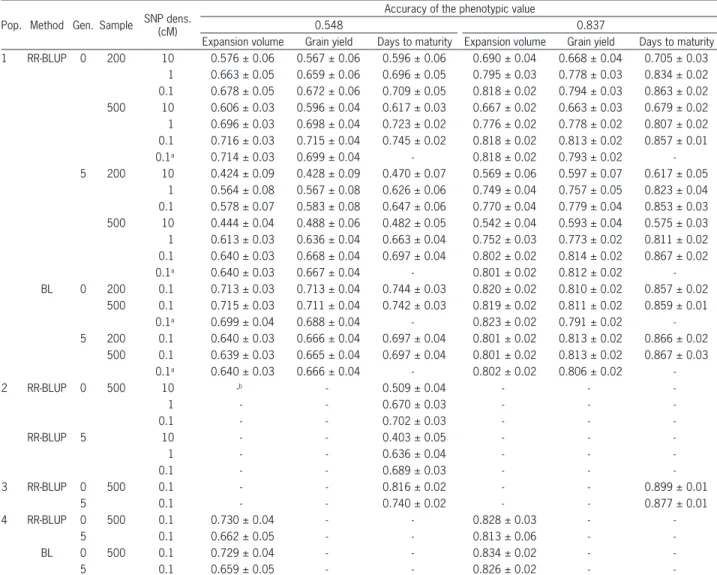
Accuracies of breeding value prediction by the RR-BLUP and BL methods were comparable, regardless of the degree of dominance, heritability, sample size and generation (Table 1). Except for density of one SNP every
10 cM in generation 5, accuracies of the breeding value prediction based on SNPs surpassed the prediction ac-curacy of phenotypic values, in the case of heritability of 0.3 (Table 1). With heritability of 0.7 and assuming dom-inance, accuracies of breeding value prediction based on markers were lower than accuracy of phenotypic values. However, except for lower density of SNPs, differences were always smaller than 20 %.
For a given heritability, regardless of generation, sample size and density of SNPs, there was no differ-ence in the breeding value prediction accuracy based on SNPs for expansion volume (bidirectional dominance), grain yield (positive dominance) and days to maturity (no dominance) (Table 1). Accuracy was raised with the increase of heritability from 0.3 to 0.7, regardless of the other factors. The average increase in accuracy was 15
Table 1 − Prediction accuracy of breeding value and its standard deviation, for expansion volume, grain yield and days to maturity in populations 1 to 4, regarding two accuracies of the phenotypic value, three SNP densities, two sample sizes and two generations, based on the BLUP and Bayesian methods
Pop. Method Gen. Sample SNP dens. (cM)
Accuracy of the phenotypic value
0.548 0.837
Expansion volume Grain yield Days to maturity Expansion volume Grain yield Days to maturity 1 RR-BLUP 0 200 10 0.576 ± 0.06 0.567 ± 0.06 0.596 ± 0.06 0.690 ± 0.04 0.668 ± 0.04 0.705 ± 0.03
1 0.663 ± 0.05 0.659 ± 0.06 0.696 ± 0.05 0.795 ± 0.03 0.778 ± 0.03 0.834 ± 0.02 0.1 0.678 ± 0.05 0.672 ± 0.06 0.709 ± 0.05 0.818 ± 0.02 0.794 ± 0.03 0.863 ± 0.02 500 10 0.606 ± 0.03 0.596 ± 0.04 0.617 ± 0.03 0.667 ± 0.02 0.663 ± 0.03 0.679 ± 0.02 1 0.696 ± 0.03 0.698 ± 0.04 0.723 ± 0.02 0.776 ± 0.02 0.778 ± 0.02 0.807 ± 0.02 0.1 0.716 ± 0.03 0.715 ± 0.04 0.745 ± 0.02 0.818 ± 0.02 0.813 ± 0.02 0.857 ± 0.01
0.1a 0.714 ± 0.03 0.699 ± 0.04 - 0.818 ± 0.02 0.793 ± 0.02
-5 200 10 0.424 ± 0.09 0.428 ± 0.09 0.470 ± 0.07 0.569 ± 0.06 0.597 ± 0.07 0.617 ± 0.05 1 0.564 ± 0.08 0.567 ± 0.08 0.626 ± 0.06 0.749 ± 0.04 0.757 ± 0.05 0.823 ± 0.04 0.1 0.578 ± 0.07 0.583 ± 0.08 0.647 ± 0.06 0.770 ± 0.04 0.779 ± 0.04 0.853 ± 0.03 500 10 0.444 ± 0.04 0.488 ± 0.06 0.482 ± 0.05 0.542 ± 0.04 0.593 ± 0.04 0.575 ± 0.03 1 0.613 ± 0.03 0.636 ± 0.04 0.663 ± 0.04 0.752 ± 0.03 0.773 ± 0.02 0.811 ± 0.02 0.1 0.640 ± 0.03 0.668 ± 0.04 0.697 ± 0.04 0.802 ± 0.02 0.814 ± 0.02 0.867 ± 0.02
0.1a 0.640 ± 0.03 0.667 ± 0.04 - 0.801 ± 0.02 0.812 ± 0.02
-BL 0 200 0.1 0.713 ± 0.03 0.713 ± 0.04 0.744 ± 0.03 0.820 ± 0.02 0.810 ± 0.02 0.857 ± 0.02 500 0.1 0.715 ± 0.03 0.711 ± 0.04 0.742 ± 0.03 0.819 ± 0.02 0.811 ± 0.02 0.859 ± 0.01
0.1a 0.699 ± 0.04 0.688 ± 0.04 - 0.823 ± 0.02 0.791 ± 0.02
-5 200 0.1 0.640 ± 0.03 0.666 ± 0.04 0.697 ± 0.04 0.801 ± 0.02 0.813 ± 0.02 0.866 ± 0.02 500 0.1 0.639 ± 0.03 0.665 ± 0.04 0.697 ± 0.04 0.801 ± 0.02 0.813 ± 0.02 0.867 ± 0.03
0.1a 0.640 ± 0.03 0.666 ± 0.04 - 0.802 ± 0.02 0.806 ± 0.02
-2 RR-BLUP 0 500 10 -b - 0.509 ± 0.04 - -
-1 - - 0.670 ± 0.03 - -
-0.1 - - 0.702 ± 0.03 - -
-RR-BLUP 5 10 - - 0.403 ± 0.05 - -
-1 - - 0.636 ± 0.04 - -
-0.1 - - 0.689 ± 0.03 - -
-3 RR-BLUP 0 500 0.1 - - 0.816 ± 0.02 - - 0.899 ± 0.01
5 0.1 - - 0.740 ± 0.02 - - 0.877 ± 0.01
4 RR-BLUP 0 500 0.1 0.730 ± 0.04 - - 0.828 ± 0.03 -
-5 0.1 0.662 ± 0.05 - - 0.813 ± 0.06 -
-BL 0 500 0.1 0.729 ± 0.04 - - 0.834 ± 0.02 -
-5 0.1 0.659 ± 0.05 - - 0.826 ± 0.02 -
-aAdditive-dominance model; bnon-simulated; SNP = single nucleotide polymorphisms; RR-BLUP = ridge regression best linear unbiased prediction; BL = Bayesian
and 26 % for generations 0 and 5, respectively, com-pared to an increase of 53 % in accuracy of the pheno-typic value. The decrease in LD due to five generations of random mating caused, as theoretically expected, a decrease in accuracy that was inversely proportional to SNP density, heritability and sample size. Regardless of the trait, with heritability of 0.3, the average decreases in accuracy were 23 and 9 % for lower and higher densi-ties, respectively. The corresponding values were 14 and 1 % with high heritability.
Accuracy decreased by less than 10 % with the decrease in the number of genotyped and phenotyped individuals (Table 1). Regardless of trait, heritability, generation, and sample size, the results showed that the approach to maximum accuracy is asymptotic. Increas-ing density from one SNP every 10 cM to one SNP every cM caused an increase in accuracy between 15 and 19 % for generation 0, and between 27 and 41 % for genera-tion 5. However, the increase from one SNP every cM to one SNP every 0.1 cM led to an increase between 2 and 7 %, regardless of the generation.
The additive and additive-dominance models pro-vided the same breeding value prediction accuracy, re-gardless of trait, heritability, and generation (Table 1). Under the same experimental condition, accuracies in similar populations regarding LD and genetic variability tend to be equivalent, regardless of trait, generation, and density of SNPs (data not shown). However, accuracies in populations with contrasting genetic variability (1 and 3) or LD (1 and 2) tend to be different under a low den-sity of SNPs (Table 1). Because additive variance is 49 % higher in population 3 (generation 0), compared to popu-lation 1, accuracy is greater, although the increase was only 10 % due to high density of SNPs. Because LD is lower in population 2 compared to population 1, breed-ing value prediction accuracies in generations 0 and 5 are 17 % and 16 % lower in lower density of SNPs, re-spectively. In higher SNP densities, the maximum differ-ence was 7 % in generation 0. Finally, we found that the RR-BLUP and BL methods are also comparable when there are few QTLs of higher effect (Table 1).
Discussion
Even taking into account that populations under-going recurrent selection cannot have the average LD and magnitude of genetic variability of the composites used in this study, when heritability is 0.3, genomic se-lection tends to be up to 25 % more efficient than pheno-typic selection depending on LD and additive variance, assuming at least 500 individuals genotyped and density of one SNP every cM. The relative efficiency should be greater with heritability lower than 0.3. When heritabil-ity is 0.7 and assuming the same conditions, the genomic selection may be up to 10 % less efficient than phenotyp-ic selection, also depending on LD and additive variance. Inferiority should be greater for heritability greater than 0.7. Therefore, efficiency of genomic selection in relation
to phenotypic selection is inversely proportional to heri-tability. For Muir (2007), genomic selection works very well for traits with low heritability, whereas for a highly heritable trait, accuracy of the breeding value prediction cannot exceed accuracy of phenotypic values. Moser et al. (2009) showed that accuracies of dairy bull breeding values predicted from 7,372 SNPs were approximately 1.3 times larger than accuracy of phenotypic selection based on progeny testing. Simulated and empirical stud-ies have systematically shown higher prediction accura-cy of genomic selection relative to phenotypic selection (Campos et al., 2013).
Because accuracy of genomic selection is affected by genetic variability in the population, efficiency of genomic selection, as phenotypic selection, is also pro-portional to additive variance in the population. Assum-ing an infinitesimal model with equal or unequal QTL variance, Bastiaansen et al. (2012) observed a greater de-crease in accuracy of breeding value prediction in gen-erations 1 to 10 under selection, based on marker effects predicted in the reference population (generation 0). This was true regardless of the method for prediction of marker effects. For the authors, the decrease in accuracy was largely due to reduction in genetic variance. Any change in LD patterns may have played a minor role. Regarding the influence of LD on accuracy of breeding value prediction, with low heritability, even after five generations of random mating without selection, muta-tion, and migration (with LD decreases of 47 and 36 % in cases of one SNP every 1 and 0.1 cM, respectively), accuracy of genomic selection is equivalent to that of phenotypic selection, regardless of trait and sample size, especially with a density of at least one SNP every cM. Solberg et al. (2009) showed that a density of eight mark-ers every cM seems sufficient for the estimated marker effects to persist over five generations with minimum bias and only a small reduction in genomic selection ac-curacy.
phe-notypic selection. Combs and Bernardo (2013) observed that greater sample size increased prediction accuracy, however, increases were lower than 20 %. Based on a deterministic approach, Grattapaglia and Resende (2011) concluded that sample size has a relatively minor impact on genomic selection accuracy. Using 1000 individuals for genotyping and phenotyping, the expected accuracy would range from 0.7 to 0.9 at high marker densities (20 markers every cM).
The approach to maximum genomic selection ac-curacy is asymptotic in relation to marker density as observed by Meuwissen et al. (2001), Grattapaglia and Resende (2011) and Combs and Bernardo (2013). Con-sidering that 100 QTLs were controlling the traits, effi-ciency of genomic selection compared to phenotypic se-lection with low density of SNPs (one SNP every 10 cM, on average) is rather surprising. This outstanding result is due solely to the fact that the population had high LD and should not be understood to imply an appropriate density for every population. Because LD declines fast along the genome, there is no doubt that genomic selec-tion should be made based on high SNP density. High SNP density is available for humans and some impor-tant animal and plant species such as cattle and maize and will soon be available for all species because with modern high-throughput genotyping and sequencing technologies, breeders can easily reach a high number of SNPs (for example, using genotyping by sequencing (Elshire et al., 2011)). Because increases in prediction ac-curacy based on density of one SNP every 0.1 cM rela-tive to accuracy of prediction with density of one SNP every cM were less than 10 % in populations with high LD, genomic selection can be efficiently applied assum-ing density of one SNP every cM in populations with high LD.
In non-inbred open-pollinated populations, predic-tions of breeding values based on additive and additive-dominance models are equivalent, especially in the RR-BLUP method. Regarding dominance effects, Toro and Varona (2010) showed an increase in the expected re-sponse to selection and in accuracy of breeding value prediction. Accuracy increases ranged from 2 to 12 % and were proportional to the degree of dominance and heritability. Wellmann and Bennewitz (2012) observed an increase of only 2 % in accuracy of breeding value prediction. Furthermore, dominance slowed down the decrease of accuracies in subsequent generations.
Based on our results, the RR-BLUP and BL meth-ods can be considered equivalent even if the model is not infinitesimal, that is, when there are QTLs of higher ef-fect, although the BL method is more suitable for smaller sample sizes. Campos et al. (2009) concluded that BL is adequate for performing regressions on markers, at least under an additive model. In the study of Crossa et al. (2010), RR-BLUP predictions of wheat lines and maize inbreds were outperformed by BL predictions. Bayesian LASSO with different variances showed the highest ac-curacies and the lowest biases for the predicted breeding
values in the study of Legarra et al. (2011). Heslot et al. (2012) recommended the RR-BLUP and BL methods for genomic selection in plant breeding. Both methods pro-vided the same accuracy of predicting breeding values regardless of species, population structure, and marker type.
Based on the huge amount of theoretical and em-pirical evidence that genomic selection is an efficient selection process irrespective of trait heritability (Dae-twyler et al., 2013) and that genomic selection has ap-plication in all breeding procedures, such as prediction of hybrid performance (Massman et al., 2013), and con-sidering that modern high-throughput genotyping and sequencing technologies will be available to an ever de-creasing cost (Campos et al., 2013), genomic selection is expected to be applied by plant breeders in almost every practical scenario.
Finally, we highlight our main theoretical and applied results on genomic selection. After 15 years since the advent of genomic selection, our theory is the most comprehensive approach on genetic funda-ments of this quantitative genetics methodology. This study shows parametric values of the average effect of SNP substitution, SNP dominance deviation and SNP additive and dominance variances, for any number of QTLs in LD with each SNP. We proved that weighted and unweighted (by SNP frequencies) estimators of the breeding value have the same accuracy. In a further study, we will present a theoretical approach for addi-tive-dominance with epistasis model, focusing on dom-inance, epistatic and genotypic values prediction. Our results applied to cross-pollinated species breeding evi-denced that RR-BLUP and BL are equivalent for breed-ing value prediction, genomic selection tends to be up to 10 % less efficient than phenotypic selection, under high heritability, and up to 25 % more efficient under low heritability and that breeding value prediction ac-curacy is not influenced by the dominance degree and is proportional to heritability, SNP density and sample size, and inversely proportional to the LD degree. Since these results have been observed in the context of for-estry and animal breeding, we emphasize that genomic selection can be efficiently applied in a recurrent selec-tion program by phenotyping and genotyping the same individuals, using as few as 200 parents and density of one SNP by cM.
Acknowledgments
References
Bastiaansen, J.W.M.; Coster, A.; Calus, M.P.L.; Arendonk, J.A.M. van; Bovenhuis, H. 2012. Long-term response to genomic selection: effects of estimation method and reference population structure for different genetic architectures. Genetics Selection Evolution 44: 3.
Campos, G. de los; Hickey, J.M.; Pong-Wong, R.; Daetwyler, H.D.; Calus, M.P.L. 2013. Whole-genome regression and prediction methods applied to plant and animal breeding. Genetics 193: 327-345.
Campos, G. de los; Naya, H.; Gianola, D.; Crossa, J.; Legarra, A.; Manfredi, E.; Weigel, K.; Cotes, J.M. 2009. Predicting quantitative traits with regression models for dense molecular markers and pedigree. Genetics 182: 375-385.
Combs, E.; Bernardo, R. 2013. Accuracy of genomewide selection for different traits with constant population size, heritability, and number of markers. The Plant Genome 6: 1.
Crossa, J.; Campos, G. de los; Pérez, P.; Gianola, D.; Burgueño, J.; Araus, J.L.; Makumbi, D.; Singh, R.P.; Dreisigacker, S.; Yan, J.; Arief, V.; Banziger, M.; Braun, H.J. 2010. Prediction of genetic values of quantitative traits in plant breeding using pedigree and molecular markers. Genetics 186: 713-724.
Daetwyler, H.D.; Calus, M.P.L.; Pong-Wong, R.; Campos, G. de los; Hickey, J.M. 2013. Genomic prediction in animals and plants: simulation of data, validation, reporting, and benchmarking. Genetics 193: 347-365.
Elshire, R.J.; Glaubitz, J.C.; Sun, Q.; Poland, J.A.; Kawamoto, K.; Buckler, E.S.; Mitchell, S.E. 2011. A robust, simple genotyping-by-sequencing (GBS) approach for high diversity species. PLoS ONE 6:e19379.
Endelman, J.B. 2011. Ridge regression and other kernels for genomic selection with R package rrBLUP. The Plant Genome 4: 250-255.
Gianola, D.; Campos, G. de los; Hill, W.G.; Manfredi, E.; Fernando, R. 2009. Additive genetic variability and the Bayesian alphabet. Genetics 183: 347-363.
Goddard, M. 2009. Genomic selection: prediction of accuracy and maximization of long term response. Genetica 136: 245-257. Goddard, M.E.; Hayes, B.J. 2007. Genomic selection. Journal of
Animal Breeding and Genetics 124: 323-330.
Grattapaglia, D.; Resende, M.D.V. 2011. Genomic selection in forest tree breeding. Tree Genetics & Genomes 7: 241-255. Heslot, N.; Yang, H.P.; Sorrells, M.E.; Jannink, J.L. 2012. Genomic
selection in plant breeding: a comparison of models. Crop Science 52: 146-160.
Hill, W.G.; Robertson, A. 1968. Linkage disequilibrium in finite populations. Theoretical and Applied Genetics 38: 226-231. Jannink, J.L.; Lorenz, A.J.; Iwata, H. 2010. Genomic selection in
plant breeding: from theory to practice. Briefings in Functional Genomics 9: 166-177.
Kempthorne, O. 1957. An Introduction to Genetic Statistics. Iowa State University Press, Ames, IA, USA.
Legarra, A.; Granié, C.R.; Croiseau, P.; Guillaume, F.; Fritz, S. 2011. Improved Lasso for genomic selection. Genetics Research 93: 77-87.
Massman, J.M.; Gordillo, A.; Lorenzana, R.E.; Bernardo, R. 2013. Genomewide predictions from maize single-cross data. Theoretical and Applied Genetics 126: 13-22.
Meuwissen, T.H.E.; Hayes, B.J.; Goddard, M.E. 2001. Prediction of total genetic value using genome-wide dense marker maps. Genetics 157: 1819-1829.
Moser, G.; Tier, B.; Crump, R.E.; Khatkar, M.S.; Raadsma, H.W. 2009. A comparison of five methods to predict genomic breeding values of dairy bulls from genome-wide SNP markers. Genetics Selection Evolution 41: 56.
Muir, W.M. 2007. Comparison of genomic and traditional BLUP-estimated breeding value accuracy and selection response under alternative trait and genomic parameters. Journal of Animal Breeding and Genetics 124: 342-355.
Park, T.; Casella G. 2008. The Bayesian LASSO. Journal of the American Statistical Association 103: 681-686.
Pérez, P.; Campos, G. de los; Crossa, J.; Gianola, D. 2010. Genomic-enabled prediction based on molecular markers and pedigree using the Bayesian linear regression package in R. The Plant Genome 3: 106-116.
Solberg, T.R.; Sonesson, A.K.; Woolliams, J.A.; Ødegard, J.; Meuwissen, T.H.E. 2009. Persistence of accuracy of genome-wide breeding values over generations when including a polygenic effect. Genetics Selection Evolution 41: 53.
Toro, M.A.; Varona, L. 2010. A note on mate allocation for dominance handling in genomic selection. Genetics Selection Evolution 42: 33.
Viana, J.M.S. 2004. Quantitative genetics theory for non-inbred populations in linkage disequilibrium. Genetics and Molecular Biology 27: 594-601.