Evaluation of Penman-Monteith model applied to a maize field in the arid area of Northwest China

(1)

HESSD

7, 461–491, 2010

Evaluation of Penman-Monteith

model

W. Zhao et al.

Title Page

Abstract Introduction

Conclusions References

Tables Figures

◭ ◮

Back Close

Full Screen / Esc

Printer-friendly Version

Interactive Discussion

Hydrol. Earth Syst. Sci. Discuss., 7, 461–491, 2010 www.hydrol-earth-syst-sci-discuss.net/7/461/2010/ © Author(s) 2010. This work is distributed under the Creative Commons Attribution 3.0 License.

Hydrology and Earth System Sciences Discussions

This discussion paper is/has been under review for the journal Hydrology and Earth System Sciences (HESS). Please refer to the corresponding final paper in HESS if available.

Evaluation of Penman-Monteith model

applied to a maize field in the arid area of

Northwest China

W.-Z. Zhao1,2, X.-B. Ji1,2, E.-S. Kang1, Z.-H. Zhang1,2, and B.-W. Jin1,2

1

Heihe Key Laboratory of Ecohydrology and Integrated River Basin Science, Cold and Arid Regions Environmental and Engineering Research Institute, Chinese Academy of Sciences, Lanzhou, 730000, China

2

Linze Inland River Basin Comprehensive Research Station, Chinese Ecosystem Research Network, Lanzhou, 730000, China

Received: 18 December 2009 – Accepted: 5 January 2010 – Published: 21 January 2010 Correspondence to: W. Zhao (zhaowzh@lzb.ac.cn)

(2)

HESSD

7, 461–491, 2010

model

W. Zhao et al.

Title Page

Tables Figures

◭ ◮

Back Close

Full Screen / Esc

Abstract

The Penman-Monteith (P-M) model has been applied to estimate evapotranspiration in terrestrial ecosystem widely in the world. As shown in many studies, bulk canopy re-sistance is an especially important factor in the application of P-M model. In this study, the authors used the Noilhan and Planton (N-P) approach and Jacobs and De Bruin

5

(J-D) approach to express the bulk canopy resistance. The application of P-M mode to a maize field with two approaches in the arid area of Northwest China was evaluated by the measured half-hourly values from the eddy covariance system. The results in-dicate that the N-P approach underestimates slightly the bulk canopy resistance, while the J-D approach overestimates that. The estimation of bulk canopy resistance with

10

N-P approach was then better and more consistent than that with J-D approach dur-ing the entire maize growdur-ing season. Corresponddur-ingly, the P-M model with J-D bulk canopy resistance slightly underestimated the latent heat flux throughout the maize growing season, but overestimated the latent heat flux during the dry period of the soil as compared to that with N-P approach. The good fitness of the simulated latent heat

15

flux by the P-M model with N-P bulk canopy resistance approach to the measured one at a half-hour time step demonstrates the application of the approach is reasonable in the relative homogenous and not drought-stressed maize fields of the arid areas during the entire growing season. Further researches are discussed on enhancing the field observation, taking the correction for atmospheric stability into estimating aerodynamic

20

resistance, to improve the performance of P-M model to simulate evapotranspiration in the cropped fields.

1 Introduction

Evapotranspiration (ET) is a principal component of the hydrological cycle in terrestrial

ecosystems, affected by both biophysical and environmental processes at the interface

25

(3)

HESSD

7, 461–491, 2010

model

W. Zhao et al.

Title Page

Tables Figures

◭ ◮

Back Close

Full Screen / Esc

1996; Baldocchi and Meyers, 1998). It serves as a regulator of the key ecological pro-cesses by linking stomatal activity, carbon exchange and water use (V ¨or ¨osmarty et al., 1998), and by linking energy balance and water balance of natural and agricultural ecosystems (Molina et al., 2006).

Quantification of water loss by ET is of primary importance for monitoring, survey

5

and management of water resources in various spatial scales of a farm scale, a catch-ment and a region (Lecina et al., 2003; Molina et al., 2006). For arid regions, ET estimation is extremely important to assess water resources. The arid inland area of Northwest China in the hinterland of Eurasia consists of various relatively independent inland river basins. Water resources in an inland basin originate from the Mountains

10

at the upperstream, controlling the vegetation distribution in the basin (Ji et al., 2006; Kang et al., 2007). The extremely limited water resources are mostly utilize by the artificial oases in the middlestream plain area, where irrigated agriculture is very de-veloped and forms a farmland ecosystem of inland river basin. The over-exploitation of

water resources at the middlestream area reduces the runoffto the downstream area,

15

causing the degradation of natural ecosystems there (Ji et al., 2006; Kang et al., 2007; Jia et al., 2009). Therefore, rational utilization and allocation of water resources is ex-tremely important in an inland river basin. This requires accurate estimation of water budget for the agriculture fields, and ET estimation is the key factor of the water loss in the budget.

20

To quantify the actual ET of crop fields at the instantaneous, hourly and daily scales, several ET models have been developed and tested in various ecosystems under the

different climatic conditions over the world (Penman, 1948; Monteith, 1965; Priestley

and Taylor, 1972; Shuttleworth and Wallace, 1985; Schmugge and Andr ´e, 1991; Kite, 2000). Among the models, the most widely used one is the physically based

Penman-25

(4)

HESSD

7, 461–491, 2010

model

W. Zhao et al.

Title Page

Tables Figures

◭ ◮

Back Close

Full Screen / Esc

parameter in modeling the actual ET of crop filed using PM model.

Two types of canopy resistance (or conductance) models have been used to express the behavior of the canopy resistance: the Jarvis type model and Ball type. The former relates the canopy resistance to environmental variables at an atmospheric reference height (Javis, 1976; Noilhan and Planton, 1989), the latter correlates canopy resistance

5

to the assimilation rate (Ball et al., 1987; Leuning, 1995; Jacobs and De Bruin, 1997). Although these two type models have been applied to various canopies and plants (Niyogi and Raman 1997; Ronda et al., 2001), there has been no comparison of the two type models to be applied in P-M model to simulate the actual ET of crop fields, especially in the arid area of Northwest China. The functions and parameters of the

10

models have yet to be evaluated in di_fferent studies and in the di_fferent environmental

conditions.

This paper is intended to compare these two types of canopy resistance models with measured canopy resistance derived from an inverted PM model; to evaluate the P-M

model with different canopy resistance approaches on modeling actual

evapotranspi-15

ration of the irrigated crop fields under arid climate; to discuss the variation of ET from

maize field during different stages of growing season, to support the water-saving

agri-culture and to improve the irrigation efficiencies of the oases in the inland river basins

of Northwestern China.

2 Evapotranspiration modeling

20

2.1 The Penman-Monteith model

The Penman-Monteith model describes the physical process of evapotranspiration from a vegetative surface, and typically can be written as:

λE=∆(Rn−G)+ρaCp(es−ea)/ra ∆ +γ(1+rs/ra)

(5)

HESSD

7, 461–491, 2010

model

W. Zhao et al.

Title Page

Tables Figures

◭ ◮

Back Close

Full Screen / Esc

whereλis latent heat of vaporization of water (MJ kg−1); E is crop evapotranspiration

(mm s−1);∆is gradient of the water saturation vapour pressure curve (kPa K−1);Rnis

net radiation (W m−2);G is soil heat flux (W m−2); ρa and Cp are the density (kg m

−3

)

and specific heat (MJ kg−1K−1) of air, respectively; es and ea are the saturated and

actual vapour pressure of air (kPa), respectively;γis psychrometer constant (kPa K−1);

5

ra is resistance to the turbulent transfer of vapour between source and the reference

level (s m−1);rsis the canopy resistance (s m

−1

).

The aerodynamic resistance was estimated by Monin-Obukhov similarity, assuming neutral conditions, by

r_a=ln[(z−d)/z0]ln[(z−d)/(hc−d)]

k2 ·

1

u (2)

10

where z (m) is the reference level at which the horizontal wind speed u (m s−1) is

measured;d is the zero plane displacement height (m), and is taken equal to 0.67 hc

(Brutesaert, 1982); z0 is the roughness length for momentum (m), approximated as

0.123h_c (Brutesaert, 1982); h_c is the height of the crop (m); k is the von Karman’s

constant, equal to 0.41.

15

2.2 The bulk canopy resistancerc

Certain environmental (Jarvis, 1976) and plant physiological (Ball et al., 1987) factors

affect the bulk canopy resistance. These factors reflect atmospheric conditions, soil

moisture, the assimilation of plant at the canopy scale and so on. Two types of bulk

canopy resistance models have been applied to expressrc: Noilhan-Planton approach

20

(6)

HESSD

7, 461–491, 2010

model

W. Zhao et al.

Title Page

Tables Figures

◭ ◮

Back Close

Full Screen / Esc

2.2.1 The parameterization of Nilhan-Planton (N-P) approach

The Noilhan-Planton bulk canopy resistancersis a function of incoming solar radiation,

mean volumetric water content, vapor pressure deficit of the atmosphere, air tempera-ture and leaf area index (Noilhan and Planton, 1989); it is given by:

rs=

rsmin

LAIF1F

−1 2 F

−1 3 F

−1

4 (3)

5

wherersmin is the minimum stomatal resistance (s m

−1

), the typical values forrsmin in

growing crops range between 40 and 100 s m−1 and for mature crops between 250

and 500 s m−1(Tattari et al., 1995). In this study, during the different stage of the maize

growing season from the initial, through development and midseason, and to the late

period, the field observation indicate that the value of rsmin was 70 s m

−1

, 70 s m−1,

10

50 s m−1, and 100 s m−1for the respective stage. LAI is the leaf area index (−);F1and

F4express the dependence ofrcon solar radiation and on air temperature, respectively;

F3 describes the dependence on the atmospheric vapour pressure deficit and F2 is

a function of soil moisture. The parameterization of Noilhan-Planton approach is given as follows (Noilhan and Planton, 1989):

15

F1=

1+f

f+r_smin/r_smax (4)

F2=

        

1, w2> wwilt

w2−wwilt

wcr−wwilt

, wwilt≤w2≤wcr

0, w2< wwilt

(5)

F3=1−β(es(Ts)−ea) (6)

(7)

HESSD

7, 461–491, 2010

model

W. Zhao et al.

Title Page

Tables Figures

◭ ◮

Back Close

Full Screen / Esc

with

f=0.55 RG

R_GL

2

LAI (8)

where rsmin is the maximum stomatal resistance (s m

−1

), and was arbitrarily set to

5000 s m−1 (Noilhan and Planton, 1989); w2 is the mean volumetric water of the soil

column (m3m−3); wcr is the soil water content below which transpiration is stressed

5

by soil moisture, taken as 0.65wsat; wwilt is the plant permanent wilting point. In this

study, the saturated soil water contentwsat is set as 0.40 m

3

m−3 and wilting point as

0.11 m3m−3for sandy loam in the field. Tsand Taare the surface and air temperature

at the crop height level (K).βis a species-dependent empirical parameter and set to

0.001 hPa−1 for maize in this study. RG is the incoming solar radiation (W m

−2

), and

10

RGLis the limit value of 100 W m

−2

for crops (Noilhan and Planton, 1989).

2.2.2 Parameterization of the Jacobs-De Bruin (J-D) model

The Jacobs-De Bruin model (Jacobs and De Bruin, 1997) is based on plant physiology, which uses a correlation relationship between the leaf stomatal conductance and the net photosynthetic rate at leaf scale, and then up-scaling the conductance from a leaf

15

to acanopy:

1/rs=

ZLAI

0

[1.6An/(Cs−Ci)]d L (9)

whereAn is the net photosynthetic rate (mg m

−2

s−1);Cs andCiare the CO2

concen-tration at the leaf surface and in the sub-stomatal cavity (mg m−3), respectively;Lis the

leaf-area index (−), which sums to LAI, the total leaf area index over the entire canopy

20

depth.

In the Jacobs-De Bruin model, the net photosynthetic rate at leaf scale is given by

An=(Am+Rd)

1−exp

₋_ε

iI

Am+Rd

(8)

HESSD

7, 461–491, 2010

model

W. Zhao et al.

Title Page

Tables Figures

◭ ◮

Back Close

Full Screen / Esc

where Am is the photosynthetic rate at infinite light intensity (mg m

−2

s−1); Rd is the

rate of dark respiration (mg m−2s−1); ε_i is the initial light use efficiency (mg J−1), I is

the amount of photosynthetically active radiation (W m−2) . Here, Rd is estimated as

0.11Am. The response ofAmto CO2is modeled as

Am=Am,max

n

1−e−[gm(Ci−Γ₎_/A

m,max]

o

(11)

5

whereA_m,max is the maximal primary productivity under light conditions and high CO2

concentrations (mg m−2s−1),gmis the mesophyll conductance (mm s

−1

), and_Γ is the

CO2compensation point (mg m

−3

).

The parameters gm,Am,max and Γ are the functions of leaf temperature Tc (K) and

computed as:

10

X(Tc)=

X(Tsk=298)Q

(T_c−298)/10 10

1+e0.3(T1−Tc) 1+e0.3(Tc−T2)

(12)

Γ(Tc)= Γ(Tsk=298K)Q

(Tc−298)/10

10 (13)

whereX denotesgmorAm,max, andT1andT2are reference temperature (K).T1andT2

forgm are set as 286 K and 309 K, respectively, while forAm,maxare set as 286 K and

311 K, respectively. As in the Jacobs-De Bruin model, the values ofgm(Tsk=298) and

15

A_m,max (Tsk=298) are set as 17.5 mm s −1

and 1.7 mg m−2 s−1 for maize, respectively;

the values ofQ10is set as 2.0 for maize;Γ(Tsk=298 K) andQ10 are set as 4.3ρaand

1.5 for maize, respectively.

In Eq. (10) the light use efficiencyεiis a function ofCs,Γ, and the initial (at low light

conditions) light use e_fficiencyε0(Jacobs and De Bruin, 1997):

20

εi=ε0

Cs−Γ

Cs+2Γ

(9)

HESSD

7, 461–491, 2010

model

W. Zhao et al.

Title Page

Tables Figures

◭ ◮

Back Close

Full Screen / Esc

The parameter values forε0 is have been derived by Collatz et al. (1991, 1992). The

value for maize (C4plant) is set as 0.014 mg J

−1

.

In laboratory experiments the internal CO2 concentration Ci is often found to be

a fraction of the external CO₂ concentration (Ronda et al., 2001). Zhang and

Nobel (1996) proposed the following formula to express the relationship between

5

(Ci−Γ)/(Cs−Γ) and the water vapour deficit:

Ci−Γ

Cs−Γ

=f0−adDs (15)

wheref0 and ad are empirically found as regression coefficients. Typical values are

f₀=0.85 anda_d=0.015 Kpa−1 for C₄ plants, respectively (Jacobs and De Bruin, 1997;

Ronda et al., 2001);Dsis the vapour pressure deficit at plant level (kPa).

10

3 Site description and field measurements

3.1 Site description

This work was carried out at the fields of maize crop during the growth season of 2008,

where is the agricultural water saving experimental plot (1 km×1 km) of Linze Inland

River Basin Comprehensive Research Station (39◦20′N, 100◦08′E, elevation 1378 m),

15

Chinese Ecosystem Research Network, Cold and Arid Regions Environmental and Engineering Research Institute, Chinese Academy of Sciences. The site is located in the central area of the Zhangye irrigation oases at the middle streams of the Heihe River, which is an inland river in the arid area of Northwest China. The terrain was relatively flat (its mean slope in the vicinity of site ranged between 2.1 and 4.5%) and

20

the maize canopy extended for over a kilometer in all directions.

The site is characterized by a typical continental arid climate, dry and hot in summer,

cold in winter. The normal annual mean air temperature is 7.6◦C, with an absolute

(10)

HESSD

7, 461–491, 2010

model

W. Zhao et al.

Title Page

Tables Figures

◭ ◮

Back Close

Full Screen / Esc

is 117 mm, with the nearly 70% concentrated in the months from July to September.

Mean annual pan evaporation is 2390 mm. Mean annual wind velocity is 3.2 m s−1, and

prevailing wind direction is northwest (Ji et al., 2007, 2009). The soil is belongs to the sandy loam type (sand: 59.0%; silt: 36.3%; clay: 4.7%). The staple crop is maize in the oasis. The surface irrigation districts account for 95% of the total irrigated area,

5

and mainly by means of the border irrigation.

3.2 Field measurements

Continuous measurements were carried out at the study site during the maize growth season from 26 May to 30 September 2008. Eddy covariance technique was used to measure the fluctuations of wind speed, temperature, carbon dioxide and water vapour

10

above the canopy. The eddy covariance system consists of a three dimensional (3-D) sonic anemometer (HS-50, Gill Solent Istruments, Lymington, Hampshire, UK) and an open-path infrared gas analyzer (LI-7500, LI-COR Inc., Lincoln, NE, USA). Vari-ances and covariVari-ances were calculated from the 20 Hz raw data. Vertical fluxes of mo-mentum, sensible heat, carbon dioxide and water vapour were determined by means

15

of 1) the three dimensional (3-D) sonic anemometer to sample the three components of

wind speed (u,v,w) and virtual acoustic temperature (the speed of sound)T and 2) an

open-path infrared gas analyzer for measurement of water vapour and carbon dioxide mole densities above the crop field. The fast response sensors were mounted at height 2 m above the crop canopy level (i.e. the sensor height varied during the measurement

20

campaigns) (Kaimal and Finnigan, 1994). The open sides of the asymmetric sonic anemometers were exposed to the north-west at the experimental plot. The open-path infrared gas analyzer were mounted 0.2 m below the sonic anemometer and displaced 0.3 m laterally and perpendicular to the predominating wind direction in order to min-imize flux loss due to vertical (Kristensen, et al., 1997) and longitudinal (Massman,

25

2000) sensor separation, respectively. Data were recorded on a Personal Computer inside of a small hut, 50 m apart.

(11)

HESSD

7, 461–491, 2010

model

W. Zhao et al.

Title Page

Tables Figures

◭ ◮

Back Close

Full Screen / Esc

software (Kolle and Rebmann, 2007) for post-processing software EDDYSOFT (Kolle and Rebmann, 2007). Half-hourly mean eddy fluxes over the crop field were calcu-lated as the covariance between turbulent fluctuations of the vertical wind speed and the scalar mixing rations calculated by Reynolds averaging of 30-min blocks of data. Following the recommendations of McMillen (1988), a 2-D coordinate rotation was

ap-5

plied to force the average vertical wind speed (w) to zero and to align the horizontal

wind (u) to mean wind direction. Both the CO₂ flux and latent flux were corrected for

density effects by the method described by Webb et al. (1980). As a result, latent and

sensible heat fluxes were calculated as:

λEEC=λ(1+χv) w′c ′ v+

c_v

T H ρcp

!

(16)

10

H=ρcpw′T′ (17)

where EEC is water vapor flux (mmol m

−2

s−1); χv is the ratio of vapour pressure to

atmospheric pressure (−);cv is the molar concentration of water vapor (mmol m

−3

);H

is sensible heat flux (W m−2); T is the sonic temperature (K);ρ is density of moist air

(kg m−3); Overbars denote time averages and primes denote the departures. Positive

15

fluxes indicate mass and energy transfer from the surface to the atmosphere, and negative from the atmosphere to the surface.

The eddy covariance technique is limited by missing or rejected measurements due to system failures, maintenance and calibration, and improper weather conditions. In this study, the following gap-filling procedures were employed: the short gaps less than

20

6 h were filled by linear interpolation. The large gaps were filled were filled by means of the look-up table approach or, if not possible, by the by the mean diurnal variation method (Falge et al., 2001).

The EVINS Environmental Monitoring System (IMKO micromodultechnik GnbH, Ett-lingen, Germany) was mounted about 60 m from the eddy covariance tower in this

(12)

HESSD

7, 461–491, 2010

model

W. Zhao et al.

Title Page

Tables Figures

◭ ◮

Back Close

Full Screen / Esc

study field. Net radiation and photosynthetically active radiation (PAR) were mea-sured by a CNR-1 net radiometer (Kipp & Zonen, Delft, The Netherlands) and a LI-190 quantum sensor (LI-COR Inc., Lincoln, NE, USA) at 2 m above the canopy. Air temperature, relative humidity, air pressure and wind speed and direction were mea-sured at the top of the canopy by a HMP45D temperature probe (Vaisala, Helsinki,

5

Finland), HMP45D relative humidity probe (Vaisala, Helsinki, Finland), PTB100 barom-eter probe (Vaisala, Helsinki, Finland), a LISA cup anemombarom-eter (Siggelkow GmbH, Hamburg, Germany), and the Young 8100 (Siggelkow GmbH, Hamburg, Germany). Canopy temperature was measured with PS12AF1 surface Pyrometer (Keller HCM GmbH, Ibbenb ¨uren-Laggenbeck, Germany). Soil temperature and volumetric soil

wa-10

ter content were measured with the Pt100 (IMKO GmbH, Ettlingen, Germany) and the TRIME-IT (IMKO GmbH, Ettlingen, Germany). Soil temperature was measured at 5, 10, 20, 40, 80 and 120 cm depths in the soil. Soil moisture was measured at 10, 20, 50, 100, 200, 300 cm in the soil. Soil heat fluxes were measured by a HFP-01 plane probe (Hukseflux Thermal Sensors, Delft, The Netherlands) and three replicate heat

15

flux plates at 0.05 m. Precipitation was measured with the RG50 tipping bucket rainfall gauges (SEBA Hydrometrie GmbH, Gewerbestr, Germany).

The stomatal conductance was hourly measured at four levels in the canopy by a LI-COR 6400 (LI-LI-COR Inc., Lincoln, NE, USA) in the maize field for 4 days over the 2008 growing season. The levels with the leaf orientations of east, west, north and south

20

(13)

HESSD

7, 461–491, 2010

model

W. Zhao et al.

Title Page

Tables Figures

◭ ◮

Back Close

Full Screen / Esc

4 Results and discussion

4.1 Diurnal variations in stomatal conductance during the maize growing

season

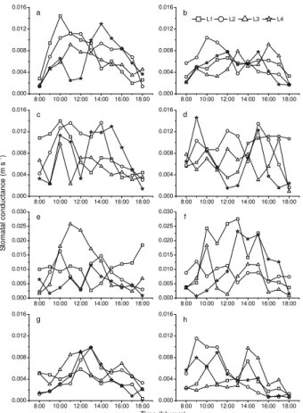
Diurnal variations in stomatal conductance was measured with a a Li-6400 for four in-dividual leaves distributing four levels in the maize canopy on selected days of growing

5

season, as presented in Fig. 1. The mean values of net radiation Rn,

photosynthet-ically active radiation PAR, air temperature at crop heightTa, vapour pressure deficit

Ds, soil water contentw2and green leaf area index LAI for the daytime (from 08:00 to

18:00 LT) of the observation days in the di_fferent stages of crop growing season are

listed in Table 1.

10

Diurnal variation in stomatal conductance has a common patterns for the different

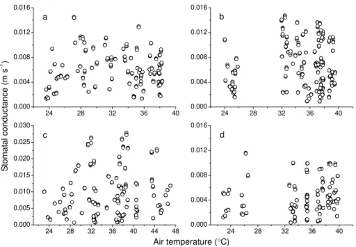
stages of maize growing season. The stomatal conductance varies with a lower value in the morning and afternoon, and a higher value in the midday, depending on solar radiation and vapour pressure deficit. The response of stomatal conductance to vapour pressure deficit, photosynthetically active radiation and air temperature is, respectively

15

showed in Figs. 2–4. This reflects a common characteristics in conductance for water to exchange between the plant and atmosphere at both the leaf and canopy scales. The diurnal variation in leaf stomatal conductance of maize in this study filed has the higher values in the morning than those in the afternoon, and lower values in midday (13:00 LT) than those before and after about 13:00 LT. The lower stomatal conductance

20

during the afternoon and midday should be attributed to the higher water vapor deficit (midday depression of photosynthesis). A lower stomatal conductance in the midday can be explained by a limitation of photosynthesis, due to the stomatal closure, to prevent the water loss from the most intensive solar radiation and higher temperature. However, the time for the lower values of stomatal conductance to occur varies with the

25

growing orientation, which influences the absorption of global radiation.

(14)

HESSD

7, 461–491, 2010

model

W. Zhao et al.

Title Page

Tables Figures

◭ ◮

Back Close

Full Screen / Esc

mean values of stomatal conductance were measured to be 5.90 mm s−1on DOY 130,

7.21 on DOY 162, 9.26 on DOY 195 and 4.29 on DOY 229, respectively. This indicates that the stomatal conductance increases with increasing PAR and decreases VPD.

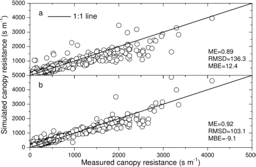
4.2 Test of the J-D and N-P approaches in the determination of the canopy

resistance

5

In order to test the J-D and N-P approaches applied to determine the bulk canopy resistance, the half-hourly bulk canopy resistance derived from P-M model based on the measured ET from the eddy covariance system was compared with that simulated by J-D (a) and N-P (b) approaches. Taking the P-M model derived bulk canopy resis-tance as the measured value, the statistical tests were performed for the comparison

10

by model efficiency (ME), root mean square deviation (RMSD) and mean bias error

(MBE) (Flerchinger et al., 2003; Ji et al., 2009).

For J-D approach, the values of ME, RMSD and MBE between the measured and

simulated bulk canopy resistance were 0.89, 136.3 s m−1and 12.4 s m−1, respectively

(Fig. 5a). Compared with J-D approach, N-P approach performances better in

simu-15

lating canopy bulk canopy resistance with the values of ME 0.92, RMSD 103.1 s m−1

and MBE −9.1 s m−1. From the MBE given in Fig. 5, it can be seen that the J-D

ap-proach overestimated the bulk canopy resistance. Therefore, the N-P apap-proach is more suitable than the J-D approach to simulate the bulk canopy resistance of the irrigated maize filed under the arid climatic condition.

20

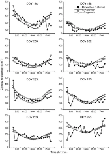
4.3 Diurnal variation in the bulk canopy resistance

In order to investigate the effect of irrigation, days were selected before and after

ir-rigation, then the daily variation of the bulk canopy resistance was simulated by the two approaches for the days and is shown in Fig. 6. During the entire maize growing season, eight times of surface irrigation (i.e., small level-basin irrigation) were totalized

25

(15)

HESSD

7, 461–491, 2010

model

W. Zhao et al.

Title Page

Tables Figures

◭ ◮

Back Close

Full Screen / Esc

variation in the bulk canopy resistance on days before and after irrigation were simu-lated on DOY 157, DOY 201, DOY 234 and DOY 254, respectively. The mean values of the meteorological and ecological elements in the daytime (from 8:00 to 18:00 LT)

on the selected days before and after irrigation applied during the different stages of

maize growth season are listed in Table 2.

5

Half-hourly values of bulk canopy resistance exhibited a reverse parabolic pattern,

reaching the maximum value near mid-day (13:00 LT) during the different stages of

maize growing season. The values were higher in the morning and afternoon, and lower at the midday, depending on solar radiation. The daily variation of resistance in-dicates that evapotranspiration increases with net radiation. It is found that, except the

10

condition of low soil water content, the bulk canopy resistance is larger in the morning than that in the afternoon (Fig. 6). This is due to both the increase of water vapour deficit and the more intensive solar radiation (or PAR) in the afternoon.

Figure 6 indicates that both J-D and N-P approaches overestimated the bulk canopy resistance in the morning and afternoon of the sunny day. Under the dry soil

condi-15

tion before irrigation, the J-D approach overestimated the bulk canopy resistance in the midday, while the N-P approach underestimated that. When soil was wet after irrigation, both approaches got the overestimated values. However, the bulk canopy resistance of maize filed simulated by N-P approach was better fitted with that derived from P-M model as compared to the J-D approach.

20

4.4 Simulation of evapotranspiration

Figure 7 presents the comparison between the measured half-hourly latent heat flux by eddy covariance system and the simulated ones by P-M model with J-D (Fig. 7a) and N-P (Fig. 7b) approaches during the maize growing season in 2008. In Fig. 7, all the measured and simulated latent heat fluxes are distributed around the one-to-one

25

line. The values of ME, RMSD and MBE were 0.67, 78.1 W m−2 and −40.3 W m−2

for J-D approach, and 0.80, 60.8 W m−2and 15.2 W m−2 for N-P approach. The

(16)

HESSD

7, 461–491, 2010

model

W. Zhao et al.

Title Page

Tables Figures

◭ ◮

Back Close

Full Screen / Esc

approaches were generally well fitted to the measured fluxes by the eddy covariance system. But, it is also important to note that the N-P approach performed better than the J-D approach.

4.5 Diurnal variation of latent heat flux

Figure 8 shows the diurnal variation in the half-hourly measured and simulated latent

5

heat flux corresponding to the data presented in Fig. 6. The latent heat fluxes reach the maximum value near mid-day. For both bulk canopy resistance approaches, the simulated and the measured daily variations of latent heat fluxes were rather well fitted. Nevertheless, the J-D approach slightly underestimated the latent heat flux during the maize growing season. The P-M model with N-P bulk canopy resistance approach

10

tended to overestimate the latent heat flux under the dry soil condition (on DOY 156, DOY 200, DOY 233 and DOY 253), and to underestimate slightly the latent heat flux under the wet soil condition. This should be attributed to the overestimations of the

bulk canopy resistance by J-D approach. However, the difference between the values

obtained with J-D and N-P approaches were generally small for both dry and wet soil

15

conditions (DOY 253 and DOY 255).

The maize field for this study was sufficiently supplied with water, and the soil water

content were generally above 0.27 (from the field measurement by the authors), below which transpiration is restricted by soil moisture. This indicates that the P-M model with J-D and N-P approaches can be applied in the relative homogenous and irrigated

20

agricultural fields as studied in this paper. On the other hand, Fig. 8 also indicates that the performance of P-M model with J-D bulk canopy approach was better than that with N-P approach when soil was dry before irrigation, and inversely is the case when soil was wet after irrigation.

Although the P-M model with J-D and N-P bulk canopy resistance approaches seems

25

(17)

HESSD

7, 461–491, 2010

model

W. Zhao et al.

Title Page

Tables Figures

◭ ◮

Back Close

Full Screen / Esc

was better than with J-D approach during the maize growing season in the oases at the middle reaches of the Heihe River basin, Northwest China.

It should be noted that the simplicities of the P-M model, such as the adequate fetch above canopy measurements, regarding canopy as a big leaf assumption, and using Monin-Obukhov similarity to estimate the aerodynamic resistance with the assumption

5

of neutral stability, affect the performance of P-M model. For instance, during early

growing season, crops are sparse and the big leaf assumption is not valid for them. The assumption of neutral stability in estimating the aerodynamic resistance is very

preliminary approximation. Further, the canopy variables are very difficult to obtain.

Among them, the determination of leaf stomatal resistance is the most difficult, which

10

is the most important parameter for J-D and N-P approaches. All these aspects need further investigations and studies.

5 Conclusions

The present study indicates that the J-D and N-P approaches can provide more realistic estimation of the bulk canopy resistance under well-watered and slightly soil moisture

15

stressed conditions at a half-hourly time step during the maize growth season. How-ever, the N-P approach seems to slightly underestimate the bulk canopy resistance. On the other hand, the J-D approach tends to overestimate these values. Meantime, it is worth noting that the performance of N-P approach was better than that of J-D approach in this study.

20

The P-M model simulation indicates that the P-M model with J-D approach slightly underestimated the latent heat flux during the maize growing season. In contrast, the P-M model with N-P approach tended to overestimate the latent heat flux under the dry soil condition, and underestimated slightly the latent heat flux under the wet soil condition. The P-M model with J-D and N-P approaches simulated latent heat well

25

(18)

HESSD

7, 461–491, 2010

model

W. Zhao et al.

Title Page

Tables Figures

◭ ◮

Back Close

Full Screen / Esc

approach is better than that with J-D approach to simulate latent heat flux at half-hourly time step during the growing season in the conditions of the relative homogenous and not drought-stressed maize field for the present study.

Further developments are necessary to make the model and approaches more ap-plicable, in particular enhancing the instrumentation under the various soil moisture

5

situations and climatic conditions during the different stages of maize growing season.

This is helpful in optimizing the parameterization of both J-D and N-P bulk canopy re-sistance approaches, and will contribute to improve the performance of P-M model to simulate evapotranspiration of cropped field in this study. Moreover, the aerodynamic resistance should be corrected for atmospheric stability to obtain better simulation of

10

evapotranspiration.

Acknowledgements. This research was supported by the National Natural Science Foundation of China (No. 40930634; 40801014), the Talent Training Program for Young Scientist in West China from the Chinese Academy of Sciences (No. 828981001), the Major State Basic Re-search Development Program of China (973 Program) (No. 2009CB421302). The data used in

15

the paper are provided by the CAS Action Plan for West Development Program (No. KZCX2-XB2-09) and Chinese State Key Basic Research Project (No. 2007CB714400).

References

Allen, R. G., Pruitt, W. O., Wright, J. L., Howell, T. A., Ventura, F., Snyder, R., Itenfisu, D., Steduto, P., Berengena, J., Yrisarry, J. B., Smith, M., Pereira, L. S., Raes, D, Perrier, A.,

20

Alves, I., Walter, I., and Elliott, R.: A recommendation on standardized surface resistance for hourly calculation of reference ET₀by the FAO56 Penman-Monteith method, Agr. Water Manage., 81, 1–22, 2006.

Baldocchi, D. and Meyers, T.: On using eco-physiological, micrometeorological and biogeo-chemical theory to evaluate carbon, dioxide, water vapor and trance gas fluxes over

vegeta-25

tion: a perspective, Agr. Forest Meteorol., 90, 1–25, 1998.

(19)

HESSD

7, 461–491, 2010

model

W. Zhao et al.

Title Page

Tables Figures

◭ ◮

Back Close

Full Screen / Esc

Interactive Discussion Progress in Photosynthesis Research: Proceedings of the Seventh International Congress

on Photosynthesis, edited by: Biggins, J., Martinus-Nijhoff Publishers, Dordrecht, The Netherlands, 221–224, 1987.

Brutsaert, W.: Evaporation into the Atmosphere: Theory, History, and Application, Kluwer, Boston, 299 pp., 1982.

5

Collatz, G. J. J., Ball, J. T., Grivet, C., and Berry, J. A.: Physiological and environmental reg-ulation of stomatal conductance, photosynthesis and transpiration: a model that includes a laminar boundary layer, Agr. Forest Meteorol., 92, 73–95, 1991.

Collatz, G. J. J., Ribas-Carbo, M., and Berry, J. A.: Coupled photosynthesis-stomatal conduc-tance model for leaves of C₄plants, Aust. J. Plant Physiol., 19, 519–538, 1992.

10

Falge, E., Baldocchi, D. D., Olson, R., Anthoni, P., Aubinet, M., Bernhofer, C., Burba, G., Ceule-mans, R., Clement, R., and Dolman, H.: Gap filling strategies for long term energy flux data sets, Agr. Forest Meteorol., 107, 71–77, 2001.

Jacobs, C. M. J. and De Bruin, H. A. R.: Predicting regional transpiration at elevated atmo-spheric CO₂: influence of the PBL-vegetation interaction, J. Appl. Meteorol. Clim., 36, 1663–

15

1675, 1997.

Jarvis, P. G.: The interpretation of the variations in leaf water potential and stomatal conduc-tance found in canopies in the field, Philos. T. Roy. Soc. B., 273, 593–610, 1976.

Ji, X. B., Kang, E. S., Chen, R. S., Zhao, W. Z., Zhang, Z. H., and Jin, B. W.: The impact of the development of water resources on environmental in arid inland river basin of Hexi region,

20

Northwestern China, Environ. Geol., 50, 793–801, 2006.

Ji, X. B., Kang, E. S., Chen, R. S., Zhao, W. Z., Zhang, Z. H., and Jin, B. W.: A mathematical model for simulating water balances in cropped field experiment under conventional flood irrigation in arid inland of Northwestern China, Agr. Water Manage., 87, 337–346, 2007. Ji, X. B., Kang, E. S., Zhao, W. Z., Zhang, Z. H., and Jin, B. W.: Simulation of heat and water

25

transfer in a surface irrigated, cropped sandy soil, Agr. Water Manage., 96, 1010–1020, 2009.

Jia, Y., Ding, X., Qin, C., and Wang, H.: Distributed modeling of landsurface water and energy budgets in the inland Heihe river basin of China, Hydrol. Earth Syst. Sci., 13, 1849–1866, 2009,

30

http://www.hydrol-earth-syst-sci.net/13/1849/2009/.

(20)

HESSD

7, 461–491, 2010

model

W. Zhao et al.

Title Page

Tables Figures

◭ ◮

Back Close

Full Screen / Esc

Interactive Discussion Kang, E. S., Lu, L., and Xu, Z. M.: Vegetation and carbon sequestration and their relation

to water resources in an inland river basin of Northwest China, J. Environ. Manage., 85, 702–710, 2007.

Kite, G.: Using a basin-scale hydrological model to estimate crop transpiration and soil evapo-ration, J. Hydrol., 229, 59–69, 2000.

5

Kolle, O. and Rebmann, C.: Eddysoft, Documentation of a Software Package to Acquire and Process Eddy Covariance Data, Jena, Technical Reports, Max-Planck-Institut f ¨ur Biogeo-chemie 10, 85–88, 2007.

Kristensen, L., Mann, J., Oncley, S. P., and Wyngaard, J. C.: How close is close enough when measuring scalar fluxes with displaced sensors, J. Atmos. Ocean. Tech., 14, 814–821, 1997.

10

Leuning, R.: A critical appraisal of a combined stomatal-photosynthesis model for C₃ plants, Plant Cell Environ., 18, 339–355, 1995.

Lecina, S., Mart´_ınez-Cob, A., P ´erez, P. J., Villalobos, F. J., and Baselga, J. J.: Fixed versus var-ialble bulk canopy resistance for referance evapotranspiration estimation using the Penman-Monteith equation under semiarid conditions, Agr. Water Manage., 60, 181–198, 2003.

15

Massman, W. J.: A simple method for estimating frequency response corrections for eddy covariance systems, Agr. Forest Meteorol., 104, 185–198, 2000.

McMillen, R. T.: An eddy correlation technique with extended applicability to non-simple terrain, Bound.-Lay. Meteorol., 43, 231–245, 1988.

Molina, J. M., Mart´ınez, V., Gonz ´alez-Real, M. M., and Baille, A.: A simulation model for

pre-20

dicting hourly pan evaporation from meteorological data, J. Hydrol., 318, 250–261, 2006. Monteith, J. L.: Evaporation and environment, in: Proceedings of the 19th Symposium of the

Society for Experimental Biology, Cambridge University Press, New York, USA, 205–233 pp., 1965.

Monteith, J. L. and Unsworth, M. H.: Principles of Environmental Physics, Edward Arnold Press,

25

London, 291 pp., 1990.

Niyogi, D. S. and Raman, S.: Comparison of four different stomatal resistance schemes using FIFE observations, J. Appl. Meteorol. Clim., 36, 903–917, 1997.

Noilhan, J. and Planton, S.: A simple parameterization of land surface processes for meteoro-logical Models, Mon. Weather Rev., 117, 536–549, 1989.

30

Penman, H. L.: Natural evaporation from open water, bare soil and grass, P. Roy. Soc. A, 193, 120–146, 1948.

(21)

HESSD

7, 461–491, 2010

model

W. Zhao et al.

Title Page

Tables Figures

◭ ◮

Back Close

Full Screen / Esc

Interactive Discussion using large-scale parameters, Mon. Weather Rev., 100, 81–92, 1972.

Rana, G., Katerji, N., and Mastrorilli, M.: Environmental and soil-plant parameters for modeling actual crop evapotranspiration under water stress conditions, Ecol. Model., 101, 363–371, 1997.

Ronda, R. J., de Bruin, H. A. R., and Holtslag, A. A. M.: Representation of the canopy

conduc-5

tance in modeling the surface energy budget for low vegetation, J. Appl. Meteorol. Clim., 40, 1431–1444, 2001.

Schmugge, T. J. and Andr ´e, J. C.: Land Surface Evaporation Measurement and Parameteriza-tion, Springer, New York, 116 pp., 1991.

Sellers, P. J., Randall, D. A., Collatz, G. J., Berry, J. A., Field, C. B., D azlich, D. A., Zhang, C.,

10

Collelo, G. D., and Bounoua, L.: A revised land surface parameterization (SiB2) for atmo-spheric GCMs. Part I: model formulation, J. Climate, 9, 676–705, 1996.

Shuttleworth, W. J. and Wallace, J. S.: Evaporation from sparse crops – an energy combination theory, Q. J. Roy. Meteor. Soc., 111, 839–855, 1985.

Tattari, S., Ikonen, J. P., and Sucksdorff, Y.: A comparison of evapotranspiration above a barley

15

field on quality tested Bowen ratio data and Deardorffmodeling, J. Hydrol., 170, 1–14, 1995. V ¨or ¨osmarty, C. J., Federer, C. A., and Schloss, A. L.: Potential evaporation functions

com-pared on US watersheds: possible implications for global-scale water balance and terrestrial ecosystem modeling, J. Hydrol., 207, 147–169, 1998.

Webb, E. K., Pearman, G. I., and Leuning, R.: Correction of flux measurements for density

20

effects due to heat and water vapor transfer, Q. J. Roy. Meteor. Soc., 106, 85–100, 1980. Widmoser, P.: A discussion on and alternative to the Penman-Monteith equation, Agr. Water

Manage., 96, 711–721, 2009.

Zhang, H. and Nobel, P. S.: Dependency of ci/ca and leaf transpiration e_fficiency on the vapour pressure deficit, Aust. J. Plant Physiol., 23, 561–568, 1996.

(22)

HESSD

7, 461–491, 2010

model

W. Zhao et al.

Title Page

Tables Figures

◭ ◮

Back Close

Full Screen / Esc

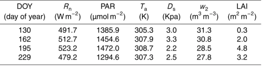
Table 1.Average daytime net radiation (Rn), photosynthetically active radiation (PAR), air

tem-perature (T_a), vapour pressure deficit (D_s), soil water content (w₂) and green leaf area index (LAI) of the observation days.

DOY Rn PAR Ta Ds w2 LAI

(day of year) (W m−2

) (µmol m−2

) (K) (Kpa) (m3m−3

) (m2m−2

)

(23)

HESSD

7, 461–491, 2010

model

W. Zhao et al.

Title Page

Tables Figures

◭ ◮

Back Close

Full Screen / Esc

Table 2. Average values of net radiation (Rn), photosynthetically active radiation (PAR), air

temperature (Ta), vapour pressure deficit (Ds), soil water content (w2), green leaf area index

(LAI), the CO₂concentration at the leaf surface (Cs) and wind speed at the reference level (u)

in the daytime on the selected days.

Rn PAR Ta Ds w2 LAI Cs u DOY

(W m−2) (µmol m−2s−1) (K) (Kpa) (m3m−3) (m2m−2) (mmol m−3) (m s−1)

156 187.7 561.2 294.8 1.6 26.4 1.6 12.1 3.1

158 382.2 1220.1 300.0 2.2 31.6 1.6 10.5 1.3

200 480.0 1410.5 301.7 2.5 26.2 4.8 12.4 1.3

202 291.6 896.3 299.5 1.7 30.9 4.8 12.4 1.2

233 464.0 1265.0 295.3 1.8 26.2 3.1 12.8 1.4

235 415.5 1028.1 297.1 2.2 32.2 3.1 12.7 1.5

253 428.1 1087.7 295.2 2.0 26.5 2.2 10.6 1.1

(24)

HESSD

7, 461–491, 2010

model

W. Zhao et al.

Title Page Abstract Introduction Conclusions References Tables Figures ◭ ◮ ◭ ◮ Back Close

Full Screen / Esc

Printer-friendly Version Interactive Discussion g f e d

8:00 10:00 12:00 14:00 16:00 18:00 0.000 0.005 0.010 0.015 0.020 0.025 0.030

8:00 10:00 12:00 14:00 16:00 18:00 0.000

0.004 0.008 0.012 0.016

8:00 10:00 12:00 14:00 16:00 18:00 0.000

0.004 0.008 0.012 0.016 8:00 10:00 12:00 14:00 16:00 18:00 0.000

0.004 0.008 0.012 0.016

8:00 10:00 12:00 14:00 16:00 18:00 0.000

0.004 0.008 0.012 0.016

L1 L2 L3 L4

8:00 10:00 12:00 14:00 16:00 18:00 0.000

0.004 0.008 0.012 0.016

8:00 10:00 12:00 14:00 16:00 18:00 0.000 0.004 0.008 0.012 0.016 b a c h S tomat a l c ondu ct a nc e (m s -1) Time (hh:mm) 1

Fig. 1. Diurnal variation in stomatal conductance in the maize canopy. The days are DOY 130

(a,b), DOY 162(c,d), DOY 195(e,f)and DOY 229(g,h). L1, L2, L3 and L4 refer to the levels at the top layer, above middle layer, below middle layer and bottom layer of the canopy. (a,c,e

(25)

HESSD

7, 461–491, 2010

model

W. Zhao et al.

Title Page

Tables Figures

◭ ◮

Back Close

Full Screen / Esc

2 4 6

0.000 0.004 0.008 0.012 0.016

0 2 4

0.000 0.004 0.008 0.012 0.016

6

0 2 4 6 8

0.000 0.005 0.010 0.015 0.020 0.025 0.030

0 2 4

0.000 0.004 0.008 0.012 0.016

6

Vapour pressure deficit (kPa)

S

tomat

a

l c

ondu

ct

a

nc

e (m

s

-1 )

a b

c d

Fig. 2. Response of stomatal resistance to vapour pressure deficit at the four levels in the

(26)

HESSD

7, 461–491, 2010

model

W. Zhao et al.

Title Page

Tables Figures

◭ ◮

Back Close

Full Screen / Esc

a b

c

0 500 1000 1500 2000 0.000

0.004 0.008 0.012 0.016

0 500 1000 1500 2000 0.000

0.004 0.008 0.012 0.016

0 500 1000 1500 2000 0.000

0.005 0.010 0.015 0.020 0.025 0.030

0 500 1000 1500 2000 0.000

0.004 0.008 0.012 0.016

Photosynthetically active radiation (µmol m-2 s-1)

S

tomat

a

l c

ond

u

c

ta

n

c

e (m

s

-1 )

d

Fig. 3.Response of stomatal resistance to photosynthetically active radiation at the four levels

(27)

HESSD

7, 461–491, 2010

model

W. Zhao et al.

Title Page

Tables Figures

◭ ◮

Back Close

Full Screen / Esc

d

24 28 32 36 40

0.000 0.004 0.008 0.012 0.016

24 28 32 36 40

0.000 0.004 0.008 0.012 0.016

24 28 32 36 40 44 48 0.000

0.005 0.010 0.015 0.020 0.025 0.030

24 28 32 36 40

0.000 0.004 0.008 0.012 0.016

S

tomat

a

l c

o

ndu

ct

a

n

c

e

(m

s

-1 )

Air temperature (°C)

a b

c

1

Fig. 4. Response of stomatal resistance to air temperature at the four levels in the maize

(28)

HESSD

7, 461–491, 2010

model

W. Zhao et al.

Title Page

Tables Figures

◭ ◮

Back Close

Full Screen / Esc

ME=0.92 RMSD=103.1 MBE=-9.1 a

0 1000 2000 3000 4000 5000

0 1000 2000 3000 4000 50000 1000 2000 3000 4000 5000

Measured canopy resistance (s m-1)

Simul

ated

c

a

nop

y

re

si

s

tan

ce

(

s

m

-1 )

b

1:1 line

ME=0.89 RMSD=136.3 MBE=12.4

Fig. 5. Comparison between measured bulk canopy resistance derived from P-M model and

(29)

HESSD

7, 461–491, 2010

model

W. Zhao et al.

Full Screen / Esc

Printer-friendly Version Interactive Discussion DOY 255 DOY 235 DOY 233 DOY 200

9:00 11:00 13:00 15:00 17:00

100 200 300 400 500

9:00 11:00 13:00 15:00 17:00

0 100 200 300 400 500

Derived from P-M model N-P approach J-D approach

9:00 11:00 13:00 15:00 17:00

0 100 200 300 400 500

9:00 11:00 13:00 15:00 17:00

0 100 200 300 400 500

9:00 11:00 13:00 15:00 17:00

0 100 200 300 400 500

9:00 11:00 13:00 15:00 17:00

0 100 200 300 400 500

9:00 11:00 13:00 15:00 17:00

0 100 200 300 400 500

9:00 11:00 13:00 15:00 17:00

0 100 200 300 400 500 DOY 158 DOY 156 DOY 202 DOY 253 Time (hh:mm) C a nopy resist an ce ( s m -1) 1

Fig. 6. Comparison of the measured and the simulated half-hourly bulk canopy resistance on

(30)

HESSD

7, 461–491, 2010

model

W. Zhao et al.

Title Page

Tables Figures

◭ ◮

Back Close

Full Screen / Esc

Interactive Discussion a

0 100 200 300 400 500 600 700

0 100 200 300 400 500 600 7000 100 200 300 400 500 600 700

Measured latent heat flux (W m-2)

Simul

at

ed

lat

e

nt heat

flux

(

W

m

-2 )

b

1:1 line

ME=0.67 RMSD=78.1 MBE=-40.3

ME=0.80 RMSD=60.8 MBE=15.2

1

Fig. 7. Comparison between the measured and the simulated half-hourly evapotranspiration

(31)

HESSD

7, 461–491, 2010

model

W. Zhao et al.

Full Screen / Esc

Printer-friendly Version Interactive Discussion DOY 255 DOY 253 DOY 233 DOY 202 DOY 200 DOY 156

9:00 11:00 13:00 15:00 17:00

0 100 200 300 400 500 600 Measured Simulated / N-P Simulated / J-D

9:00 11:00 13:00 15:00 17:00

0 100 200 300 400 500 600

9:00 11:00 13:00 15:00 17:00

0 100 200 300 400 500 600

9:00 11:00 13:00 15:00 17:00

0 100 200 300 400 500 600

9:00 11:00 13:00 15:00 17:00

0 100 200 300 400 500 600

9:00 11:00 13:00 15:00 17:00

0 100 200 300 400 500 600

9:00 11:00 13:00 15:00 17:00

0 100 200 300 400 500 600

9:00 11:00 13:00 15:00 17:00

0 100 200 300 400 500 600 Time (hh:mm) DOY 158 DOY 235 Late n t hea t fl ux ( W m -2) 1

Fig. 8.Measured and modeled courses of half-hourly latent heat flux on days before and after