E. N. Duarte
[email protected] Federal Institute of São Paulo Industrial Automation Department 12.929-600 Bragança Paulista, SP, BrazilS. A. G. Oliveira
[email protected] Federal University of Uberlandia – UFU Faculty of Mechanical Engineering 38400-902 Uberlândia, MG, BrazilR. Weyler
[email protected] Technical University of Catalonia Aeronautic Engineering 08222 Terrassa, SpainL. Neamtu
[email protected]BES La Salle International project manager 08022 Barcelona, Spain
A Hybrid Approach for Estimating the
Drawbead Restraining Force in Sheet
Metal Forming
In order to achieve better part quality in sheet metal forming the rate of the material flow into the die cavity must be efficiently controlled. This control is obtained using a restraining force supplied either by the blankholder tool, drawbeads or both. When the restraining force required is too high, the use of drawbeads is necessary, although excessive blank deformation may be produced. Some other disadvantages such as adjustment difficulties during die try-outs to determine the actual Drawbead Restraining Force (DBRF) may also be encountered. One way to solve these problems and to reduce the number of die try-outs – which are very much time consuming – is to introduce/define accurate enough drawbead concepts. The present study will make use of a method that has been developed using the similitude approach in order to understand the influence of the most important parameters on DBRF and to establish a pre-estimate DBRF theory. Data bases have been developed throughout Explicit Dynamic Finite Element Method (EDFEM) based simulations. The results are compared with experimental databases provided by Nine (1978) and with the analytical model of Stoughton (1988) results. The average of absolute error with respect to experimental data bases was around 6% and, for the studied cases, the maximum discrepancy was found to be below 11%. For the analytical and experimental cases, the average of absolute error was approximately 5% and, for the studied cases, the maximum error was below 7%. In terms of precision, the predictions derived from this approach are adequate when compared with analytical and experimental results. For this reason, the approach has been validated and accepted as a contribution to STAMPACK®, a commercial explicit dynamic finite element based system for forming processes numerical simulation.
Keywords: drawbead, restraining force, finite element method, sheet metal forming
Introduction
1
Improvement in the quality of parts obtained in sheet metal forming depends on how much adequate is the control of the material flow rate into the die cavity. This control is achieved by a restraining force supplied either by the blankholder tool, drawbeads device or both. According to Tufekci et al. (1994), when the required restraining force is too high the use of drawbeads is necessary. However, when the sheet passes through them, excessive deformations may be produced. Some other disadvantages, such as difficulties of adjustment during die try-outs in order to encounter the actual Drawbead Restraining Force (DBRF) may also be encountered. There are different kinds of causes which arise from these difficulties, for example: great variety of drawbead geometries, wide range of materials grades and several processes variables. In order to solve these problems and to reduce the number of die try-outs, which are very much time consuming, precise drawbeads concepts are necessary. For this reason a study concerning the design of drawbeads is needed in order to determine with accuracy enough the actual magnitude of this force.
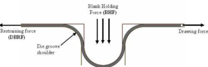
A conventional drawbead is a device which has a semi-cylindrical bead located over one binder face that fits into a die groove. The most widely used geometrical form of the drawbead cross section is circular, although rectangular, triangular, trapezoidal and unsymmetrical forms may also be found. In the current work, only the circular form is examined, (see Fig. 1), but this methodology can be easily extended to other geometries.
During the last thirty years, several authors have conducted research to better understand the forming processes and the devices used in die design, such as the drawbeads. Analytical, numerical and semi-empirical approaches have been developed. The first analytical
Paper accepted May, 2010. Technical Editor: Nestor A. Zouain Pereira
approach was developed by Swift (1948). His work was carried out considering the bending and unbending succession when the sheet passes through the drawbeads. The material was assumed to be isotropic with linear strain-hardening and strain rate-independent behavior. According to Wang (1982), Swift’s results are only applicable to a single bead and, so, he proposed a model considering a material following a strain hardening power law and anisotropy for a circular cross section bead. Nine (1978) performed experiments to study the influence of the bending deformation and friction on DBRF. His work also considered the bending and unbending succession as the sheet passes through the drawbeads. Drawing and clamping load were measured for steel and aluminum. His experimental data were discussed from the viewpoint of the materials effects, which must be taken into account in a mathematical model for drawbead forces. In the present study, Nine’s results were used as a part of the validation.
©
Figure 1. Drawbead stamping process for a circular cross section bead.
Cao and Teodosiu (1992), Chabrand and Dubois (1992) and Chabrand et al. (1992) developed models in FE to study the dynamic contact problem involving friction between the drawbeads and the sheet. Using 2D simulations, Carleer et al. (1995) established an approach by which the distributions of DBRF of the sheet are initially curve-fitted as a function of displacement so that these functions are applied as boundary conditions to produce similar effects in 3D modeling. This approach has been named the “equivalent drawbead method”.
Recently, there has been growing emphasis on Finite Element (FE) modeling in sheet metal forming. We have no doubt as to the potential of the numerical techniques. However, the three-dimensional (3D) FE simulation of complex parts forming is expensive in terms of computation. Thus, research aiming to find solutions for this problem and reducing these limitations to a more acceptable level are needed. In order to produce these results it will be necessary to reduce the required memory size and the time spent on each FE forming simulation. It is for this reason that two-dimensional (2D) FE approaches to simulate the drawbeads have been performed.
Nowadays, in practice there are industry problems with some boundary conditions or parameters range out of the approach the existent analytical models may offer. Therefore, this study was carried out aiming: to understand the influence of the most important parameters describing the DBRF behavior and to elaborate an analytical expression to pre-estimate the constraining force in a form more suitable for use in the implementation of a computer program.
This expression takes into account relevant parameters which can be divided into three main groups: geometry, material and processes parameters.
To this end, a hybrid approach has been formulated using a similitude approach (see Section 2 of this article) with data bases developed throughout explicit dynamic FE method based simulations. This procedure has been adopted after analyzing the agreement between the 2D FE drawbead simulations and Nine’s (1978) experimental results.
Nomenclature
a’ = element displacements
b = the number of considered basic dimensions B’ = bending matrix
C = constant value to be determined c = clearance
Dˆ = strength rate matrix of the flow model E = Young Modulus
F = general predictive equation F = component functions H = bead penetration K = constant hardening L = length
M = mass matrix of the structure M = mass associated with each point
n = the total number of quantities involved Rb = bead radius
Sy = conventional elastic limit
t = sheet thickness t = time
d( t )& = velocities vector
d( t )&& = acceleration vector
p[ d( t ),d( t )]& = internal forces
f [ d( t )] = external forces Cr& = damping component
d& = nodal translation velocities vector
d
&&
= nodal translation accelerations vectorGreek Symbols
cr
t
Δ = critical time t
Δ = time step employed in the integration
max
ω = maximum angular frequency
π
= Pi termμ
= friction coefficientSubscripts
S the number of Pi terms cr critical
max maximum b bead
Prediction Equations Using Similitude
The theory of similitude may be developed by dimensional analysis which involves consideration of the dimensions of the examined phenomenon. According to this theory, special attention is focused on the conditions that would permit the behavior of two separated physical systems to be treated similarly.
Accurate prediction equations may be established when the dimensional analysis is combined with experimental procedures. Aiming to develop a general prediction equation (GPE), a combination of the relations corresponding to each of the dimensionless groups may be tried as products or sums of expressions, named prediction equations. Based on dimensional analysis, it is possible to formulate an equation that involves an unknown function of dimensionless groups, which are known as Pi terms and may be written, generically, as follows:
1 2 3 4
π
=
F(
π π π
,
,
,...,
π
S)
(1)being s the number of dimensionless groups involved in the phenomenon and which may be obtained on the basis of the Buckingham Pi Theorem, as described by Murphy (1950). All Pi terms used in this paper will be described nearly.
The Buckingham Pi Theorem
The Buckingham Pi Theorem states that “the number of dimensionless and independent quantities required to express a relationship among the variables in any phenomenon is equal to the number of quantities involved minus the number of dimensions by which those quantities may be measured”, that is:
s= −n b (2)
quantity from an expression may be evaluated in terms of the dimensions F, L, and T, representing Force, Length and Time, respectively).
Let us now assume that if there are eight quantities and three dimensions involved, five Pi terms would be required, in which case we may write:
F( , , , )
π1= π π π π2 3 4 5 (3)
(see details in Murphy (1950)). It must be emphasized that the only restriction related to the Pi terms, according to Buckingham Pi Theorem, is that they must be independent and dimensionless.
Fitting Functions
The type of function which most adequately fits the phenomenon is a priori unknown. Therefore, this function must be established before formulating the general prediction equation (GPE). An analysis of the databases must be conducted by the researcher in order to determine the nature of the most suitable function. In order to determine this function, the dimensionless groups may be arranged so that all Pi terms remain constant except the one under evaluation. This procedure may be standardized and applied to each of the Pi terms. Thus, the relations identified for individual Pi terms may be combined in a general equation which represents the phenomenon. Frequently, this combination is not simple, although acceptable results may be obtained once the appropriate configuration has been established.
Combining the Functions
In order to develop the GPE, a combination of the relations corresponding to each of the Pi terms and π1 may be tried as products or sums of expressions, according Murphy (1950). At this stage, we will explain only the necessary and/or sufficient conditions needed to establish this combination.
Hypothetically, when there are three Pi terms involved in the description of a certain phenomenon, the function may be written as follows:
F( , )
π
1=π π
2 3 (4)Experiments – or simulations – would be performed varying
π2 and maintaining π3 constant, in which case an initial relationship between π1 and π2 could be obtained, as follows:
(
π
1)3= f (1π π
2, 3) (5)where the bar identifies a constant value that the researcher must define.
This procedure may also be standardized and applied to each of the Pi terms. Thus, another set of experiments would be performed – this time by keeping π2 and varying π 3 – for the second relationship to be established:
(π1)2=f (2 π π2, 3) (6)
These types of functions will be called component equations and may be combined by multiplication:
C ( ) ( )
π1= π13 π1 2 (7)
where C is a constant value to be determined.
In order to find the GPE, a multiplicative scheme may be assumed, in which case the component equations may be combined as follows:
F(π π2, 3)=f (1 π π2, 3) f (2 π π2, 3) (8)
If this is assumed to be true, then the first set of tests, with π3 constant, may be obtained as follows:
) ( )f ( f )
F(π2,π3 = 1π2,π3 2π2,π3 (8a) in which case the following may be written:
) ( f ) F( ) ( f 3 2 2 3 2 3 2
1 π π
π π π π , , , = (8b)
Performing the second set of tests withπ2kept constant in Eq. (8), we have, similarly:
) ( f ) F( ) ( f 3 2 1 3 2 3 2
2 π π
π π π π , , , = (8c)
Eq. (8b) and (8c) are substituted into Eq. (8) such as:
F( , )F( , )
F( , )
F( , )
π π π π
π π
π π
= 2 3 2 3
2 3
2 3 (8d)
Equation (8d) gives now the C value as 1F(π2,π3) to be used in Eq. (7) and also demonstrates that the two component equations must have the same form, according to Murphy (1950).
A validation procedure must be applied to the component equations, using a new data set. The same procedure must be repeated for all Pi terms in order to verify whether the general equation can be obtained as a product of the component equations. The following equation is therefore proposed:
F( , ) F( , ) F( , ) F( , )
π π π π
π π = π π
2 3 2 3
2 3 2 3
(9)
where the double bar indicates that a new set of data was used in the validation procedure with another constant value for π 2= π2.
Regardless the number of Pi terms this approach may be applied to phenomena involving more than three Pi terms, as discussed above.
It may be demonstrated that, if the component equations are combined by multiplying, the general form for the GPE, according to Murphy (1950), will be:
S S S
S
S S
F( , , ,..., )F( , , ,..., )F( , , ,..., )...
F( , , ,..., )
[ F( , , ,..., )]
π π π π π π π π π π π π
π π π π
π
π π π π −
=
3 4 2 4 2 3
2 3 4
2 3 4
2 3 4
1 2
(10) whereπ2, as well as the other pi terms kept constants, must be the same in each component group of data.
©
The Explicit Solution in FE Simulations
The general dynamic equation which describes the problem depicted in Fig. 1 may be written as:
M .d( t )&& +p[ d( t ),d( t )]& =f [ d( t )] (11)
where M is the mass matrix of the structure, d(t), d( t )& and d( t )&& are displacements, velocities and acceleration vectors, respectively;
p[ d( t ),d( t )]& represents the internal forces and f [ d( t )] the
external ones.
The differential Eq. (11) may be solved using implicit or explicit methods. The implicit solution, developed as an equilibrium problem, has often a lower computational time cost compared with the explicit one. However, in many cases when the objective is to verify the possibility of wrinkles arising and the historical information output, the explicit solution may be a more suitable option in sheet metal forming.
Memory requirements for both methods – implicit and explicit – are different: the explicit solution requires less than the implicit solution, according to NAFEMS (1992).
However, in the explicit solution case, the problem is not approached as an equilibrium problem. The configuration of the structure at the time
n n n
t+1= + Δt t+1 is determined from the known geometry of step n, using finite differences based time integration algorithm.
Explicit time integration of the Eq. (11) requires a critical time step to be respected when deforming the FEM mesh. According the STAMPACK® Theory Manual (2003), an expression used to estimate the critical time value is provided by:
2 t t
ω Δ ≤ Δ =
max
cr (12)
where max
ω is the maximum angular frequency of a discrete problem and Δtcr is the critical time. The safety coefficient applied to an estimating realized over the natural frequency is approximately 25%, according to the same reference. Δt is the time step employed in the integration of the dynamic equation and n is the number of steps used in this procedure. To illustrate a hypothetical case, an equation that describes a certain nodal translation may be obtained integrating the following expressions:
Step one:
n n n n
1
d = (f(d,t) - p(d,d) - Cr ) M
&& & & (13)
Step two:
1 1 1
2 2
1
. .( )
2 n n n
n n
d&+ =d&− + d&& Δt− + Δt (14)
Step three:
n+1 n 1 n
n+ 2
d = d + d& .Δt (15)
where d& is the nodal translation velocities vector, d&& is the nodal translation accelerations vector and Mis the mass associated with each point. The term Cr& represents the damping component.
Methodology
The principal advantage of dimensionless analysis is related to the reduction in the number of variables that influence the phenomenon. The key issue is to arrange the parameters in appropriate, dimensionless groups. As explained above, different sets of data (from every Pi term) are necessary to describe this process.
In previous studies, similitude was calculated from databases developed using experimental procedures. However, in the present research, not only experimental databases, but also numerical databases have been used to elaborate each component equation, according to either an exponential or a potential function. The experimental databases used by Nine (1978) were necessary to be referred during the final model validation.
Methods were designed with the objective of taking advantage of the promising results obtained using a 2D FEM based code to estimate the DBRF. At the same time, this approach will be used to eliminate the principal disadvantage of the explicit solution: the high computational time spent in order to achieve accurate simulations. For this purpose, an equation that estimates the DBRF is needed. This is going to be furthermore explained.
Modeling the Problem
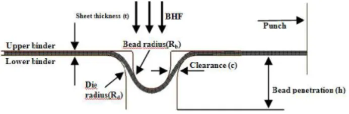
When a sheet is subjected to the force of the drawbead, a complex combination of geometrical and material factors arises from the deformation forces. Its deformation is complex because the bending of the sheet is inverted four times at punching. Tensile and compressive strains occur, simultaneously, on both sides of the sheet, varying from zero at the neutral axis, to maximum values on the sheet surface. One of the factors which affect the value of these forces is the magnitude of the local strain, Nine (1978). This is determined by the geometry of the drawbeads and the thickness of the sheet metal, (see Fig. 2).
Figure 2. The FE model of circular drawbeads.
The deformation forces are also affected by strain hardening, represented by a constitutive equation. Cyclical strain is considerably different from unidirectional increasing strain hardening. Clearance between the blankholder and the drawbeads has an important influence on the observed bending radius. If the observed radius is greater than that used in the reference shape, the bending strain will be less than calculated. It must be remembered that the magnitude of the plastic strain compared to elastic strain will determine the plasticity assumption, that is, when the phenomenon is inside the elastic zone, the small strain hypothesis can be assumed.
Finite Element Models for Achieving Simulation Databases
In order to calculate the most effective DBRF, two different 2D FE models have been designed. In the first case, as shown in Fig. 3, a sheet has been subjected to a circular drawbead between the upper binder and the die.
Figure 3 also demonstrates the blank holding force (BHF) direction, the punch stroke direction and the bead that fits into the die groove.
In order to verify the FE model response to the numerical parameters, studies about the number of elements was carried out. After this study, its mesh was structured with 240 quadrilateral elements, three of them along the sheet thickness.
Figure 3. Model 1 with suitable mesh for a circular drawbead.
Other numerical parameters, as critical time and damping coefficient, were also investigated during the FE model adjustment, with respect to the experimental data base. The optimum values encountered for them were equal to 0.00010 s and 5, respectively. See Duarte (2007), for more details.
The second model has been designed similarly to the first one, but without the drawbead, as shown in Fig. 4. The aim was to calculate only the contribution of the drawbead to the DBRF, neglecting the friction effect along the whole of its extension. This contribution is simulated in Model 2 and, subsequently, subtracted from the DBRF calculated in Model 1.
Figure 4. Model 2 with suitable mesh without the drawbead.
3-D FE simulations were also used in order to perform the adjustments of the FE model. At this stage, the validations were carried out using a new element named Basic Shell Triangle (BST), as depicted in Fig. 5. It was developed by Oñate and Zienkiewicz (1983) in order to improve its performance in terms of computational cost. For more details, see also Oñate (1997).
The BST formulation allows easily computational implementation, because only translations associated to each node are considered in the mass matrix. For this new formulation, the local velocities vector can be expressed as following:
a B
y x y x
′ ′ = ⎪ ⎭ ⎪ ⎬ ⎫
⎪ ⎩ ⎪ ⎨ ⎧ = ′
′ ′ ′ ′
γ ε ε ε
(16)
where B’ is the bending matrix; the nodal labels vector a’ brings the element displacements, as shown in Fig. 5. Using the virtual velocities principle, it was possible to find the local element stiffness matrix, as shown in Eq. (17):
∫ ′ ′ =
′
(e) A
T
dA B Dˆ B K
(17)
where Dˆ is the strength rate matrix of the flow model and B’ is the bending matrix, according to Oñate (1995).
u,v,w
Z'
y'
X'
n (c)
i
l
j
m Z
y
X
(e)
(b)
(a) k
Figure 5. Basic Triangle Shell (BST) element.
However, in the 2D FEM simulations of this research for achieving the numerical databases, the quadrilateral element used is a classic standard beam element. It was used to simulate the influence of the main parameters on the DBRF. The 2D model used to carry out these simulations is depicted in Fig. 6:
Figure 6. Details of Model 1 designed with quadrilateral elements of STAMPACK®.
In order to define the shape functions of this quadrilateral element – see Fig. 7 – it is necessary to use the beam formulation for the analysis of thin sheet metal forming, as described in details in Zienkiewicz (2004).
Figure 7. Quadrilateral sheet 2D element.
©
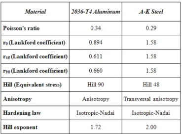
Table 1. Assumptions for material properties.
After validation procedures, the magnitude of the BHF has been obtained. This calculation included the examination of relative thickness recommended and a perfect fit of the upper bead, without clearances from the die, for both materials. The value obtained was approximately 25 kN.
The shoulders, the bead and the die radius were designed with values equal to 4.75 mm. The simulated values for stroke and velocity of the punch were 38 mm and 85 mm/s, respectively. This punch stroke was carefully calculated in order to ensure that a sheet element would pass along the full extension of the drawbead and simulate the complete process of bending, sliding and unbending the sheet.
Development of the Predictive General Equation (PGE)
To perform the PGE building process, twelve independent quantities were chosen to express the relation among nine dimensionless groups, as described in Section 2.1. Both of them (BHF and DBRF) are shown in Fig. 1. The remaining geometrical forms are available in Fig. 2 as follows: sheet thickness (t), die radius (Rd), bead radius (Rb), clearance (c) and bead penetration (h).
The material properties are taken into account by choosing those parameters assigned: Young Modulus (E), Conventional elastic limit (Sy), isotropic hardening constant (K) and isotropic hardening
exponent (n), as well as the friction coefficient (μ). After the selection of those parameters which had the most influence on the DBRF, nine Pi terms were elaborated so that the Pi theorem requirements were satisfied.
In order to reduce the number of necessary phenomenon observations the study variables were arranged in dimensionless groups. However, at least seven data points were identified for each pi term from the FE simulations. The value of each parameter was stipulated within a range determined according to the most usual values used in practical cases. π = DBRF/BHF, which is the ratio of restraining force to the blank holding force. This pi term is the dependent variable in the next relationship which involves the remaining pi terms:
π1=C. ( ). ( ). ( ). ( ). ( ) ( ). ( ). ( )f2π2 f3π3 f4π4 f5π5 f6π6 f7π7 f8π8 f9π9 (18) In Eq. (18), fi , i = 2, 3, ... , 9, are the functions used in fitting
the data achieved from FE simulations. The other pi terms are defined as follows: π2 = t/Rb is the ratio of sheet thickness (t) to
the bead radius (Rb), both in mm; π3 = μ is the friction coefficient
pi term; π4 = n is the exponent hardening coefficient; π5 = E/K is
the ratio of Young Modulus (E) to constant hardening (K), both in MPa; π6 = Sy/K correlates the conventional elastic limit (Sy) and the
constant hardening (K), both in MPa; π7 = h/Rb is the ratio of bead
height (h) and bead radius (Rb), both in mm; π8 = c/Rb correlates the
clearance (c) and the bead radius (Rb), in mm; π9 = Rd/Rb is the ratio
of the die radius (Rd) to the bead radius (Rb), both in mm.
According Murphy (1950), the constant C for nine pi terms may be written as:
1 C
Fπ π π π
=
⎡ ⎤
⎣ ⎦
7
2 3 4 9
( , , ,..., )
(19)
Proceeding with the calculations, the component equations must be obtained. As described above, the contribution of each parameter for the DBRF must be evaluated. This process has to be developed by fitting a function to the database developed based on FE simulations. At least, seven points for each Pi term have been simulated.
To ensure that only the contribution of the parameter under investigation was being evaluated, all simulations were conducted holding the remaining groups as dimensionless constants with pre estimated values. The chosen functions for fitting the databases were either the potential type as π1= 1.( )πi 2
c
c
,
or the exponential type as π = ( 4π)1 3
. . c i
c e . It must be remembered that these functions have been generated based on a multiplicative approach and for this reason it was advisable to keep them of the same nature, in order to satisfy the test outlined above. Before this procedure, however, component equations must be previously calculated. These fitted functions with their correlations for eight pairs of dimensionless groups are depicted in Figs. 8 to 15.
Regarding the applicability of the GPE obtained in this research, there are some limits to be observed in its employment: thin plates, where 0, 50≤ ≤t 2, 00 [mm] for the sheet thickness usually employed in stamping processes. In addition, predictions of GPE are more precise when made within the following parameters range:
4, 00≤ ≤h 12, 00 [mm] for height bead, 0, 00≤ ≤c 1, 50 [mm] for clearance, 75≤ ≤E 275 [GPa] for Young Modulus, 300≤K≤700 [MPa] for hardening constant and 75 650
y
S
≤ ≤ [MPa] for the conventional elastic limit. These parameters range have been chosen according to investigations about their usual values in sheet metal forming.
Figure 9. Friction component equation.
Figure 10. Hardening coefficient component equation.
Figure 11. Young modulus component equation.
Figure 12. Conventional elastic limit component equation.
Figure 13. Bead penetration component equation.
Figure 14. Clearance component equation.
Figure 15. Radii component equation.
©
Results and Discussion
In the present study, the GPE obtained by combining the best correlation component equations as a product has the following form:
5 2
b 3 4
Sy 7
m
b6 K 8 9
b b
t b
b
R b μ b n
2 3 4 5
b c R
b b
R R
6 7 8 9
b
E DBRF C BHF a e a e a e a
K
h
a e a a e a e R
⎛ ⎞
⎜ ⎟
⎜ ⎟
⎝ ⎠
⎛ ⎞ ⎜ ⎟
⎜ ⎟ ⋅ ⋅
⎝ ⎠
⎛ ⎞ ⎛ ⎞
⎜ ⎟ ⎜ ⎟
⎜ ⎟ ⎜ ⎟
⎝ ⎠ ⎝ ⎠
⎛ ⎞
= ⋅ ⋅ ⋅ ⋅ ⋅ ⋅ ⋅ ⋅ ⋅⎜ ⎟ ⋅
⎝ ⎠
⎛ ⎞
⋅ ⋅ ⋅ ⋅⎜ ⎟ ⋅ ⋅ ⋅ ⋅
⎝ ⎠
(20)
By using the numerical, geometrical and material properties parameters described in the previous sections, a closed equation was derived. It can be written using Eq. (20) and assigning to it ai and bi
constant values obtained from the component equations, in Figs. 8 to 15, which are:
4 6 8
2
2 4 6 8
3 5 7 9
3 5 7 9
a = 1,6109 a = 0,9344 a = 1,2534 a = 0,6347
b = 3,6628 b = -1,298 b = 0,5165 b = -0,5633 a = 1,0345 a = 0,8947 a = 0,9122 a = 2,8409
b = 1,2362 b = 0,0466 b = 0,4610 b = -0,9286 (21)
Subsequently, the magnitude of C must be evaluated. Using the conditions stipulated in this study, it was found that C is equal to 1.1738, thus concluding the entire process of obtaining the GPE. In practice, the final objective of the approach here applied was to derive optimum values for the constants C, ai and bi, in Eq. (20).
Testing with Experimental Data Bases
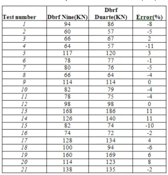
In addition to the procedures of validation and adjustment of the FE model, some tests were performed with the GPE obtained in order to investigate accuracy of its results. First, a comparison with experimental databases from Nine (1978) was examined. Table 2 brings out the comparison between Nine's results and the predictions evaluated with this current approach and their associated percentile errors.
Table 2. Tests with experimental databases of Nine (1978).
Table 3 shows the main parameters used in each experiment by Nine (1978). All experiments above listed were carried out with clearance equal to zero. For more details about methodology used in those experiments, see Nine (1978).
Table 3. Material, geometrical and process parameters from experimental databases of Nine (1978).
It is possible to be noted also that the module of average error was about 6% and, for those cases studied, the greater value of every error was never superior to 11%. From the view point of this approach, this accuracy would be improved if simulations used to fit the component equations were performed with more expensive computational costs.
Testing with an Analytical Solution
Using Levy’s model as a first approach (Levy (1983); Levy (1985)), Stoughton (1988) has developed an analytical model to pre-estimate the DBRF. The basic idea from his model was to integrate the deformation work through the sheet thickness and across the drawbead geometry, based on the virtual work principle.
Table 4. Parameters for five drawbeads. [Data available in Guo et al. (2000)].
Using the data from Table 4 and those ones described in Table 5, predictions for the DBRF were evaluated by using Stoughton and the GPE obtained in this study.
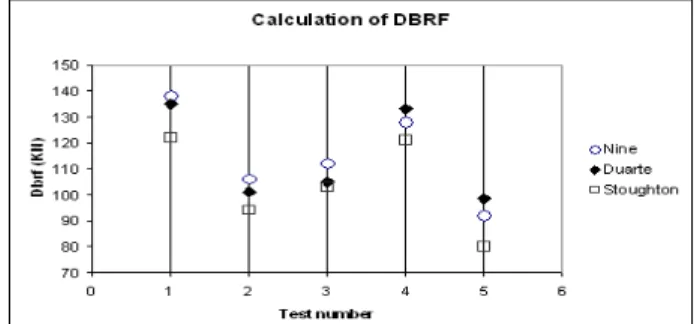
Table 5. A comparison with Stoughton and Nine's results. [Data available in Guo et al. (2000)].
It was possible to verify that the predictions made with this approach are very precise when compared with analytical and experimental results.
It was also possible to note that the module of average error was about 5% and, for the five cases studied, the maximum error was about 7%. These results are plotted in Fig. 16, to better visualization.
Figure 16. Comparison with analytical and experimental results available in Guo et al. (2000).
Conclusions
Two FEM models were designed with drawbead and without drawbead to simulate a sheet metal forming process considering the contributions of eight dimensionless groups on the DBRF – drawbead restraining force. In each case a function was fitted and used as a component equation for the methodology proposed: use of similitude in engineering with FEM based simulation data bases to determine a formulation in a closed form, in order to predict the DBRF.
Regarding the applicability of the GPE obtained in this research, there are some limits to be observed, that is: thin plates, where 0, 50≤ ≤t 2, 00 [mm] for the sheet thickness. In addition, predictions of GPE are more precise when made within the following parameters range: 4, 00≤ ≤h 12, 00 [mm] for height bead, 0, 00≤ ≤c 1, 50 [mm] for clearance, 75≤ ≤E 275 [GPa] for Young Modulus, 300≤K≤700 [MPa] for hardening constant and 75≤Sy≤650 [MPa] for the conventional elastic limit.
Predictions made with the General Prediction Equation (GPE) developed in this study were contrasted to 2D FE simulations carried out with STAMPACK®, with experimental data bases of Nine (1978) and with the analytical model of Stoughton (1988). The average of absolute error with respect to experimental data bases was about 6% and, for those cases studied, the maximum discrepancy was found to be less than 11%. For analytical and experimental investigations, the average of absolute error was about 5% and, for the five cases studied, the maximum error was about 7%.
Predictions of GPE, as it was developed in this study and within its applicability, may be considered accurate because the maximum error for these tests has been found to be less than 11% and the average of the absolute error was about 6%.
A program in FORTRAN® 90 was developed in order to determine Eq. (20) by calculating the constants C, ai and bi using the
methodology described above. Thus, Eq. (20) may be optimized in the future by achieving data from simulations with improved accuracy.
The methodology developed in this research, should permit formulation in a closed form using data obtained from simulations for drawbeads with other geometrical forms. This may be accomplished in the near future.
Acknowledgements
As a doctoral student of the Federal University of Uberlandia, E. N. Duarte wishes to acknowledge the support of CAPES – Coordenação de Aperfeiçoamento de Pessoal do Ensino Superior – of the Ministry of Education of Brazil. The authors also thank to G. Etlinger for the assistance in the edition of this paper, to CIMNE and Quantech ATZ in Barcelona, Spain, and the Instituto Fábrica do Milênio, in Brazil.
References
Cao, H.L., Teodosiu, C., 1992, “Numerical simulation of drawbeads for axisymmetric deep-drawing”. In: Numerical Methods in Industrial Forming Processes, Ed. Chenot, Wood and Zienkiewics, Balkerma, Rotterdam, pp. 439-449.
Carleer, B.D., Vreede, P.T., Drent, P., Louwes, M.F.M., Huètink, J., 1995, “Modeling drawbeads with finite elements and verification”, J. Mater. Process. Technol., Vol. 45, pp. 63-68.
Chabrand, P., Dubois, F., 1992, “Influence of the drawbead on the blankholder resulting forces”. In: Numerical Methods in Industrial Forming Processes, Ed. Chenot, Wood and Zienkiewics, Balkerma, Rotterdam, pp. 449-455.
Chabrand, P., Dubois, F., Gelin, J.C., 1996, “Modeling Drawbeads in Sheet Metal Forming”, Int. J. Mech. Sci., Vol. 38, No. 1, pp. 59-77.
Duarte, E.N., 2007, “Estudo analítico-numérico de freios de estampagem em chapas metálicas”, Doctoring Thesis, Federal University of Uberlandia, Uberlandia, Brazil. (In Portuguese)
Guo, Y.Q., Batoz, J.L., Naceur, H., Bouabdallah, S., Mercier, F., Barlet, O., 2000, “Recent developments on the analysis and optimum design of sheet metal forming parts using a simplified inverse approach”, J. Computers and Structures, Vol. 78, pp. 133-148.
Levy, B.S., 1983, “Development of a predictive model for draw bead restraining force utilizing work of nine and wang”, J. Applied Metalworking, Vol. 3, No.1, pp. 38-44.
Levy, B.S., 1985, “Modeling binder using parametric models based on mechanics considerations. In: Computer Modeling of Sheet Metal Forming Process; Theory, Verification and Application”, Eds. N.M Wang and S. C. Tang, Ann Arbor, MI, pp. 177-191.
Murphy, G., 1950, “Similitude in Engineering”. The Ronald Press Co., NY, USA, pp. 17-47.
NAFEMS, 1992, “Introduction to Nonlinear Finite Element Analysis”. Ed.: E. Hinton, 1st ed. East Kilbride, Glasgow.
©
Oñate, E., Zienkiewicz, O.C., 1983, “A viscous shell formulation for the analysis of thin sheet metal forming”, Int. J. Mech. Sci., Vol. 25, pp. 305-335.
Oñate, E., Cendoya, P., Miguel, J., 1977, “Nuevos elementos finitos para el análisis dinámico elastoplástico no lineal de estructuras laminares”, Monografia CIMNE No 36, 1997.
STAMPACK®, 2003, “Theory Manual”, Quantech ATZ S.A. Barcelona, Spain, version. 5.4.
Stoughton, T.B., 1988, “Model of drawbead forces in sheet metal forming”, Proc. 15th Biennial Congress of IDDRG, Dearborn, MI, pp. 205-215.
Swift, M.A., 1948, “Engineering”, pp. 166-333.
Tufekci, S.S., Wang, C.T., Kinzel, G.L., Altan, T., 1994, “Estimation and control of drawbead forces in sheet metal forming”, SAE Paper No. 940941.
Wang, N.M., 1982, “A mathematical model of drawbead forces in sheet metal forming”. J. Applied Metalworking, Vol. 2, No. 3, pp. 193-199.