SMEs probability of default: the case of the hospitality sector

153

SMEs probability of default: the case of the hospitality sector

Luís Pacheco

Portucalense University, Department of Economics, Management and Computer Sciences, Rua Dr. António Bernardino de Almeida, 541-619, 4200 – 072 Porto, Portugal, luisp@upt.pt

Abstract

In this paper we analyze a set of financial ratios from hospitality sector SMEs in order to ascertain which factors determine a greater probability of default. We choose the hospitality sector due to its importance in the Portuguese economy and has been particularly affected by the recent economic downturn and austerity measures and because, to the best of our knowledge, this sector has never been the object of such a study. Usually the literature seeks to find a set of variables which are significant in the estimation of default and multiple discriminant analysis and logit methodology are the main avenues of research on this area. Our data was collected from SABI and we followed logit methodology. Our results recommend that in ascertaining the creditworthiness of borrowers only debt and equity variables appear to be relevant to explaining failure, and overreliance on profit as an indication of good financial performance should be limited. The main reason for our rather poor results could be from problems with the data quality, possibly since the accounts published by firms aren’t reliable and tend to present negative results.

Keywords: Financial management, hospitality sector, SME, Logit models, default modeling.

Resumo

Neste artigo analisamos um conjunto de rácios financeiros de PME do sector hoteleiro, com o objetivo de descobrir quais os factores que determinam uma maior probabilidade de falência. Escolhemos o sector hoteleiro dada a sua importância na economia portuguesa e pelo facto de ter sido particularmente atingido pelo recente período de crise económica e pelas medidas de austeridade implementadas em Portugal. Além disso, o sector nunca terá sido alvo de um estudo deste género. Habitualmente, a literatura procura encontrar um conjunto de variáveis significativas na estimação da falência, sendo a análise múltipla discriminante e a metodologia logit os principais caminhos seguidos em termos de investigação. Os dados utilizados foram recolhidos na SABI e foi adotada a metodologia logit. Os resultados recomendam que, na aferição da qualidade de crédito dos devedores, apenas as variáveis associadas à dívida e ao capital parecem ser relevantes para explicar a falência, devendo o excesso de importância conferido aos lucros como indicador de um bom desempenho financeiro ser limitado. A principal razão para a pouca robustez dos resultados encontrados poderá ficar a dever-se à qualidade dos dados, na medida em que as contas publicadas pelas empresas sofrem de enviesamentos e aquelas tendem a apresentar resultados negativos.

Palavras-chave: Gestão financeira, sector hoteleiro, PME, Modelos logit, modelização da falência.

1. Introduction

Small and medium enterprises (SMEs) are commonly referred to as the backbone of the economy, the Portuguese case being no exception. One of the main problems reported by Portuguese SMEs is how to finance their activity, being largely dependent on banks. Also, following Basel regulations, banks need to estimate probabilities of default in order to compute minimum capital requirements. Based on these premises, the main goal of this paper is to analyze a set of financial ratios linked to the SMEs of a specific sector and ascertain which are the most predictive variables affecting individual probability of default. Therefore, considering the Portuguese hospitality sector – one of the main sectors in terms of number of firms, sales and employment – from a sample of 999 enterprises we analyze if a predefined set of factors determine a greater probability of failure.

We don’t intend to discuss the credit risk determinants and the capacity of different financial and economic ratios to forecast firm failure as there is abundant literature on that; Altman and Narayan (1997), Bonfim (2007) and Altman and Sabato (2007) being good surveys. Our main objective is to present a scoring model which is suitable to period updating and uses a set of easily available financial indicators.

The next section presents a review of the relevant literature on this subject, highlighting the main differences between Multiple Discriminant Analysis (MDA) and Logistic Regression Analysis (logit) approaches, providing a survey of the most relevant literature about failure prediction methodologies. The third section discusses the importance of SMEs in the overall economy and reasons to study the hospitality sector and section 4 presents the data, the methodology to be used and the results. The final section presents a discussion about the results and some concluding remarks about this issue.

2. Review of the relevant literature

It is well established that the effective use of screening technology greatly reduces information asymmetry between borrowers and lenders, thereby enhancing the efficiency of the finance intermediation process (Psillaki, Tsolas & Margaritis, 2010). From a credit risk perspective, SMEs are different from large corporations for many reasons. For instance, they are riskier but have a lower asset correlation with each other than large businesses do, so applying a default prediction model developed on large corporate data to SMEs will result in lower predictive power and likely a poorer performance of the entire corporate portfolio than with separate models for SMEs and large corporations (Altman & Sabato, 2007). A wide range of models has been developed for the estimation of firm

154

default probability. These models can be classified according to the type of data required. The models for pricing risky debt are based on market data, following the Merton model, and are therefore not suitable for small and unquoted enterprises. Statistical models, such as those based on discriminant analysis and binary choice models, mainly use financial-accounting ratios which are available for all enterprises regardless of their size.

During recent decades several authors have contributed to the copious literature about default prediction. The starting point was the seminal papers from Beaver (1966) and Altman (1968), who used a set of financial ratios to predict business failures. The multiple discriminant analysis (MDA) technique developed by Altman (1968) fueled the works of many authors, such as Deakin (1972), Edminster (1972), Blum (1974), Eisenbeis (1977), Taffler & Tisshaw (1977), Altman, Haldeman & Narayan (1977), Gombola, Haskins, Ketz & Williams (1987) and Lussier (1995), among others, finding that a firm is more likely to fail if it is unprofitable, highly leveraged, and suffers cash-flow difficulties. As pointed out by Altman & Sabato (2007), most of these studies violate two basic assumptions of multiple discriminant analysis – the normality of the independent variables and the equality between the variance-covariance matrices of the failing and non-failing group. Moreover, because the standardized coefficients don’t indicate the relative importance of different variables, some authors use a logit model, beginning with Ohlson (1980), which doesn’t require such restrictive assumptions. With logistic regression we can analyze a large number of relevant financial measures in order to select the most predictive ones. These variables are then used as predictors of the default event. After the paper by Ohlson (1980), which analyzed a dataset of U.S. firms over the years of 1970-1976 and estimated a logit model with nine financial ratios as regressors, most academic literature also used logit models to predict default [see inter alia Zavgren (1985), Gentry, Newbold & Whitford (1985), Keasey & Watson (1987), Aziz, Emanuel & Lawson (1988), Platt & Platt (1990), Mossman, Bell, Swartz & Turtle (1998), Becchetti & Sierra (2003)]. Focusing on SMEs, Altman & Sabato (2005) analyzed U.S., Australian and Italian SMEs separately, and Altman & Sabato (2007) used a dataset of U.S. SMEs. Lo (1986) shows that despite the theoretical difference between multivariate discriminant analysis and logistical regression the statistical results are quite similar in terms of classification accuracy and Lennox (1999) argues that a well-specified logit model can identify failing companies more accurately than discriminant analysis. Although not highlighted here, other statistical methods for building quantitative credit assessment models are; probit models, decision trees, artificial neural networks and genetic algorithms [see Wilson, Chong & Peel (1995) and Back, Laitinen, Sere & Van Wezel (1996)]. In recent times more quantitatively demanding and robust nonparametic approaches such as data envelopment analysis (Psillaki et al., 2010) and case based reasoning (Li & Sun, 2011) assess credit risk and support the credit decision process.

From a statistical point of view logit regression seems to fit the characteristics of the default prediction problem well,

where the dependent variable is binary and the groups are discrete, non-overlapping and identifiable. The logit model yields a score between zero and one which conveniently gives the probability of default. Lastly, the estimated coefficients can be interpreted separately, showing the importance of each of the independent variables in explaining the estimated probability of default.

Together with the statistical method to be used, the selection of appropriate and informative balance sheet variables is the other main issue to be tackled. Despite some differences among the papers cited above a convergence emerges on some types of financial indicators, which can be grouped into five categories: leverage, liquidity, profitability, coverage and activity (Altman & Sabato, 2007). Our analysis could naturally be improved by the use of qualitative and macroeconomic variables as predictors of failure [as demonstrated by Grunet, Norden & Weber (2005) and Altman, Sabato & Wilson (2010)]. However, the SABI database does not provide a large set of qualitative variables and many studies use a sample period that is too short to allow the incorporation of these macroeconomic effects into the model.

3. SMEs and probability of default 3.1 Relative importance of SMEs

One characteristic that has emerged as a factor in evaluating default risk is firm size. Since Ohlson (1980), several studies indicate that the size of a firm has a significant impact on its credit risk exposure, meaning that the probability of default is higher among small-sized firms and much lower in medium and large-sized ones, since the latter tend to be more highly diversified and are less vulnerable to sector-specific shocks.

In Portugal, according to the Commission Recommendation 2003/361/EC of 6 May (Decreto Lei nº. 372/2007) concerning the definition of micro, small and medium-sized enterprises:

1. The category of micro, small and medium-sized

enterprises (SMEs) is made up of firms which employ fewer than 250 persons and which have an annual turnover not exceeding EUR 50 million, and/or an annual balance sheet total not exceeding EUR 43 million.

2. Within the SME category, a small enterprise is defined as

a firm which employs fewer than 50 persons and whose annual turnover and/or annual balance sheet total does not exceed EUR 10 million.

3. Within the SME category, a microenterprise is defined as

a firm which employs fewer than 10 persons and whose annual turnover and/or annual balance sheet total does not exceed EUR 2 million.

SMEs have retained their position as the backbone of the European economy, with some 20.7 million firms accounting for more than 98 per cent of all enterprises, of which the lion’s share (92.2 per cent) are firms with fewer than ten employees. In 2012 it was estimated that European Union SMEs accounted for 67 per cent of total employment and 58 per cent of gross value added (GVA). However, the

155

current difficult economic environment continues to impose severe challenges on them.

According to INE (2014), in 2012, 99.9% of the Portuguese enterprises were SMEs, of which 96% were micro enterprises. Also, SMEs employed 78% of the employees in the private sector, accounting for 58% of the total turnover and with an average of 2.58 persons per firm.

3.2 Why study the hospitality sector?

For this type of research it is better to study a particular sector in order to control possible idiosyncrasies of different industries. With respect to Portuguese firms there are few papers published using firm-level financial data to predict probabilities of default, although some authors have developed sector-specific studies, using either multiple discriminant analysis (MDA) or logit models [some examples are Santos (2000) and Leal & Machado dos Santos (2007)]. The Portuguese hospitality sector has already been studied in terms of management accounting and control systems (Faria, Trigueiros & Ferreira, 2012), performance evaluation (Nunes & Machado, 2014) or quality certification (Soares, 2014) but to the best of our knowledge the Portuguese hospitality sector firms’ probability of default has never been studied. For instance, Martinho & Antunes (2012) perform a similar analysis for Portuguese firms, applying dummy variables to account for differences among sectors, in which the dummy for the “hospitality sector” is not significant. This scarcity is also a motive for the present research.

The Hospitality sector (CAE 55 and 56 – “Alojamento,

Restauração e similares”) represents 7.8% of the total

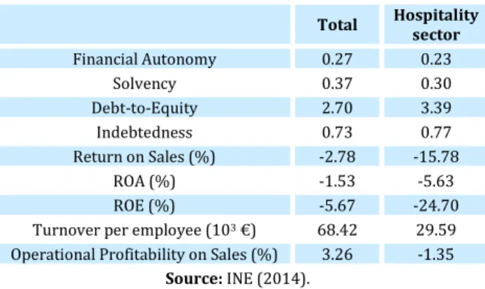
number of firms (83.103), of which 99.9% are SMEs, and of those 95.6% are micro and only 0.4% are medium enterprises. SMEs employ 88.6% of the sector total. Table 1 presents a comparison of some main financial and economic indicators for the total numbers of Portuguese SMEs and the particular case of the hospitality sector:

Table 1 - Average financial and economic indicators for SMEs

Total Hospitality _sector

Financial Autonomy 0.27 0.23 Solvency 0.37 0.30 Debt-to-Equity 2.70 3.39 Indebtedness 0.73 0.77 Return on Sales (%) -2.78 -15.78 ROA (%) -1.53 -5.63 ROE (%) -5.67 -24.70

Turnover per employee (103 _{€) 68.42 29.59} Operational Profitability on Sales (%) 3.26 -1.35

Source: INE (2014).

A simple analysis of these numbers shows a struggling sector, with higher levels of debt and lower profitability. Notice that the hospitality sector, in comparison to total SMEs, presents weaker values for all the ratios, in particular in terms of turnover per employee and profitability. In relation to demographic data, according to INE (2014), in 2012 the sector witnessed the birth of 10,582 new enterprises, which contrasts with 5,701 SME deaths registered in 2011. The birth rate in the sector is in line

with the national global average. Considering micro enterprises, the birth and death rates are both higher than the national average. These facts make the sector decidedly responsible for the creation, and also the destruction, of employment opportunities.

4. Data and methodology

4.1 Data

Our study involves a sample of 999 firms (CAE 55 and 56) taken in May 2014 from SABI, a financial database powered by Bureau van Dijk, of which 941 were “active” and 58 were considered “inactive” (these 58 occurrences were registered between 2004 and 2014). So, due to data availability, “default” means the end of the firm’s activity, that is, the status where the firm needs to liquidate its assets for the benefit of its creditors. This definition of failure includes voluntary liquidation and dissolution where there may be no risk of default, but we are unable to distinguish between voluntary and compulsory failures. We use only public data, while banks usually build their models on private data (e.g., default on single bank loans) taken from credit registers. The accounts analyzed for the companies are the last set of accounts and the n-2 and n-4 accounts. For the “inactive” firms we consider the accounts filed in the year preceding insolvency. From that first sample we choose only those SMEs with the following criteria:

 Having between 10 and 250 workers;  Having total assets lower than 43 M€;  Having a turnover lower than 50 M€ .

Note that we exclude firms with less than 10 employees because micro sizes tend to present gaps in terms of data and potential anomalous values. One of the primary issues of credit scoring research has been to determine which balance sheet variables significantly influence the probability of default (Marshall et al., 2010). In relation to the ratios to consider, in the literature there is a large number of possible candidate ratios identified as useful for predicting failure. For instance, Chen & Shimerda (1981) showed that of more than 100 financial ratios, almost 50 percent of them were found useful in empirical works. Here we follow Martinho & Antunes (2012), applying a set of six ratios defined as in Table 2 (with the corresponding expected signs):

Table 2 - Variables

Variables Definition Expected _sign

ROA Return on Assets –

TUR Earnings in percentage of total assets – FIND financial debt in percentage of total _assets + NFIND non-financial debt in percentage of _{total assets} + LIQ Cash and equivalents in percentage of _{total assets} – CAP Equity in percentage of total assets –

Source: Author.

Since these ratios are commonly used in the literature, we consider them to be a good starting point for explaining failures in the Portuguese hospitality sector.

156

After considering the criteria that define a SME, computing the six indicators for the three periods and considering only the cases with non-missing data, we ended up with 460 “active” and 25 “inactive” SMEs, representing a total turnover of 1,250 M€ (15% of the sector total) and distributed between medium and small enterprises, as can be seen in Table 3:

Table 3 - Distribution of “active” and “inactive” firms in terms of size

Medium Small Total

“Active” SMEs 180 280 460

“Inactive” SMEs 11 14 25

Source: Author.

Notice that we have a total of 485 firms of which 25 failed, which corresponds to roughly 5% – a number that

is more or less in line with the demographic average for the sector.

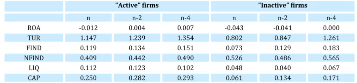
Before building and estimating the model we analyze the average values for the different indicators and for the two groups of firms. Tables 4 and 5 present descriptive statistics of the independent variables used in estimating the logit regression model as well as their distribution. As can be seen in Table 4, the “inactive” SMEs present a greater deterioration in the ratios compared with the “active” SMEs. This downgrading is clear as we approach the moment of failure, in particular for the ROA, TUR and CAP variables. Nevertheless, the “active” firms share part of that deterioration, perhaps suggesting the presence of macro drivers. Table 5 presents some information about the distribution of the financial ratios in the most recent year for which we have data.

Table 4 - Average values for the ratios in the two groups of firms

“Active” firms “Inactive” firms

n n-2 n-4 n n-2 n-4 ROA -0.012 0.004 0.007 -0.043 -0.041 0.000 TUR 1.147 1.239 1.354 0.802 0.847 1.261 FIND 0.119 0.134 0.151 0.073 0.129 0.183 NFIND 0.409 0.442 0.490 0.526 0.486 0.565 LIQ 0.112 0.123 0.102 0.048 0.040 0.067 CAP 0.250 0.282 0.293 0.061 0.134 0.171 Source: Author.

Table 5 - Distribution of the ratios in the two groups of firms

“Active” firms “Inactive” firms

ROA s.d. 0.147 0.108 p10 -0.105 -0.121 p50 0.003 -0.009 p90 0.106 0.015 TUR s.d. 1.216 0.818 p10 0.139 0.060 p50 0.779 0.665 p90 2.566 1.338 FIND s.d. 0.140 0.085 p10 0.010 0.003 p50 0.080 0.039 p90 0.249 0.159 NFIND s.d. 0.244 0.368 p10 0.134 0.220 p50 0.372 0.439 p90 0.731 0.881 LIQ s.d. 0.169 0.093 p10 0.001 0.000 p50 0.031 0.007 p90 0.390 0.178 CAP s.d. 0.409 0.457 p10 -0.018 -0.312 p50 0.302 0.087 p90 0.635 0.506 Source: Author.

Note: s.d. is the standard deviation. p10, p50 and p90 represent the 10th_{, 50}th

and 90th percentile, respectively.

The information presented in these two tables confirms economic intuition. “Active” firms typically present higher capital and liquidity ratios, lower levels of debt (except financial debt), and a greater capacity to generate earnings and returns (Table 4). For instance, ROA for “inactive” firms is -4.3%, whereas for “active” firms is -1.2%. Those differences are also observable in Table 5 which presents the standard deviation, the median and the tails of the distribution (percentiles 50, 10 and 90). As expected, the differences increase as we approach the tails of the distribution related to a negative performance. Also, the standard deviation shows a high dispersion for the different ratios. Such high variability can be due to the different ages of the firms in the sample as well as their different levels of financial health. Notice that, despite this apparent conclusion, an “inactive” firm could have better financial ratios than an “active” firm, which highlights the probability for a scoring model to over or underestimate the default probability of a particular firm (Martinho & Antunes, 2012, p. 120). Notice that simple mean comparison is not exhaustive in itself since it provides little information on cause and effect implying that ratios may have little or no ability to predict failure, in spite of differences in their means (Beaver, 1966).

The variables without a lower bound of zero (ROA and CAP) failed the normality tests for skewness and kurtosis, implying that MDA would unlikely provide satisfactory results. To further clean up the data some authors winsorize the variables, setting those observations above (below) the 99th ₍₁st_{) percentile at the value of the 99}th ₍₁st₎

percentile. Nevertheless, we confirmed that such an operation didn´t significantly change the results.

157

4.2 Methodology and results

The lack of a theory about firm bankruptcy makes prediction accuracy dependent on the best possible selection of variables included in the prediction models and also on the statistical method that is used (see Back et al., 1996).

Knowing that the process that leads a firm to bankruptcy is connected to a downgrading of its economic and financial indicators, the literature commonly uses ratios in the models, since liquidity, profitability, activity, solvency and indebtedness ratios, together with non-financial variables such as dimension and age prove to be significant in estimating the probability of default. Due to the analysed period of bankruptcy we do not incorporate macroeconomic variables typical of Macroeconomic-based models and Hybrid-models. Therefore,

the results of the model should not be sensitive to systematic macroeconomic changes not captured by the regressors used. As stated above, in this paper we follow recent work from Martinho & Antunes (2012) which uses a discrete variable model based on a logistic function:

zt = Pr ( yt = 1  xt-1 ) = _{𝟏+𝐞(−β.𝐱𝐭−𝟏)}𝟏 (1)

where yt is equal to 1 for the “inactive” firm and 0 for the

“active” firm. The z-score zt is the probability of default during

period t, conditional on the six variables presented in the previous section and which enter in xt. This specification has

the advantage of giving the probability of default directly. The model was estimated for the last year of available data and the results for the estimation are presented in Table 6.

Table 6 - Results

I II

coef. z-stat. prob. coef. z-stat. prob.

C -1.57 ** -2.29 0.02 -1.74 *** -4.82 0.00 ROA 1.74 0.96 0.34 … … … TUR -0.20 -0.66 0.51 -0.34 -1.35 0.18 FIND -6.66 ** -2.30 0.02 -6.67 ** -2.34 0.02 NFIND -0.05 -0.06 0.95 … … … LIQ -2.47 -0.93 0.35 … … … CAP -1.71 ** -2.51 0.01 -1.44 *** -3.38 0.00

p-value LR statistic statistic 0.01 0.00

McFadden R2 _{0.09 0.08}

Source: Author. Note: ***, ** and * denotes statistical significance at, respectively, 1%, 5% and 10%.

Table 6 presents the results of two alternative regressions: one with all six variables and the other without ROA, NFIND and LIQ. As is usual in binary models with micro data, the pseudo-R2 _{is low, around 9%. That means that the variability in default}

observed in the data is only partially explained by the variability of the financial ratios. Not all of the slopes (signs) are the expected ones. For instance, in regression I the signs for ROA, FIND and NFIND are puzzling, and ROA, TUR, NFIND and LIQ are not statistically significant. The results for the debt variables could be explained by the fact that, surprisingly and as we saw in Table 4, “active” firms show higher levels of financial debt to assets than “inactive” firms. Additionally, the fact that 203 firms present a negative ROA could explain the wrong sign. We note that Mata, Antunes & Portugal (2010) discuss some mechanisms that justify how the probability of default depends on the level of debt, and Appiah & Abor (2009)

raised concerns on the “over reliance” on profitability as a measure of solvency. In regression II, the sign for FIND continues to be wrong, although all the variables are statistically significant with the exception of TUR.

The high variability in the financial ratios is likely to play a strong role in these results, so following Altman & Rijker (2004) we use a logarithmic transformation for all of the six variables in order to reduce the range of possible values and increase the importance of the information given by each one of them. The variables ROA, LIQ and CAP are transformed as follows:

ROA  - Ln (1-ROA); LIQ  - Ln (1-LIQ); CAP  - Ln (1-CAP) and the other three variables have the standard log transformation. We ran two regressions after these transformations and present the results in Table 7.

Table 7 - Results (logged variables)

III IV

coef. z-stat. prob. coef. z-stat. prob.

C -3.42*** -6.30 0.00 -3.56*** -8.76 0.00 LROA 0.56 0.31 0.76 … … … LTUR -0.16 -0.77 0.44 -0.27 -1.58 0.12 LFIND -0.27*** -2.75 0.00 -0.27*** -2.71 0.01 LNFIND -0.09 -0.26 0.79 … … … LLIQ -2.05 -0.99 0.32 … … … LCAP -1.26** -1.96 0.05 -1.25*** -2.72 0.01

p-value LR statistic statistic 0.01 0.00

McFadden R2 _{0.08 0.08}

Source: Author. Note: ***, ** and * denotes statistical significance at 1%, 5% and 10%.

158

The results for regressions III and IV show a pseudo-R2

around 8%. Here the slopes for TUR, LIQ and CAP are correct but some of the variables aren’t statistically significant. Regression IV uses the variables TUR, financial debt and CAP, although TUR continues to be non-significant. In sum, only the FIND and CAP variables seem to be in some way relevant to explaining the failure.

The following table summarizes the average z-score estimated with the different models, its standard deviation and the average values for “active” and “inactive” firms. As we can see in Table 8 comparing the two types of firms, the average z-score is always higher for the “inactive” ones.

Table 8 - Average z-scores and standard deviation

I II III IV

Average z-score 0.052 0.052 0.052 0.052 Standard deviation 0.046 0.044 0.046 0.046 "Inactive" firms z-score 0.079 0.074 0.084 0.083 "Active" firms z-score 0.050 0.050 0.050 0.050

Source: Author.

We now analyze the accuracy of the different models. The performance of the default model can be measured in different ways and an exhaustive presentation of the available validation techniques can be found in BCBS (2005). A firm is considered “inactive” if, after allocating the explanatory variables to the estimated coefficients, the value of the dependent variable is greater than the cut-off-point, and otherwise is considered as “active” if that value is lower or equal. So, the number of predicted bankruptcies depends on the chosen cut-off. For example, if the cut-off point is equal to 0.10, a firm for which the expected probability of bankruptcy exceeds 10% is predicted to go bankrupt, whereas a firm for which the expected probability of bankruptcy is less than 10% is predicted to survive. Not knowing the costs of Type I and Type II errors the cut-off-point was fixed at the average z-score for “inactive” firms (Type I error means that a firm is considered as “inactive” when in fact is “active” – a false positive – and Type II error is the opposite – a false negative). Although that may not be the optimal value, the purpose of this work is to compare the prediction accuracy of the different regressions and not to find the best cut-off strategy. Notice that using a value equal to the average “inactive” z-score means that when the estimated value of the dependent variable is greater than that the firm is considered as “inactive”. Table 9 presents the error rates for the four different regressions. It should be noted that they are apparent error rates that should be treated with caution, since they are the result of the application of the model.

Table 9 - Misclassification rates and accuracy ratios

Type I error Type II error Accuracy ratio

I 18.7% 44.0% 68.7%

II 18.3% 48.0% 66.9%

III 12.6% 48.0% 69.7%

IV 13.9% 60.0% 63.0%

Source: Author.

Table 9 presents the following: the first column shows the Type I error rate, that is, the percentage of “active” firms classified as “inactive”; the second column shows the Type II error rate, that is, the percentage of “inactive” firms classified as “active” and the third column shows an index which measures the accuracy of each model in correctly classifying “inactive” and “active” firms (computed as the complement of the simple average of the Type I and Type II error rates). As can be seen in the table, the model accuracy tends to be rather low, albeit classifying the majority of the different firms correctly (better than a random process). The average accuracy ratio is above 67 percent and we see a higher prevalence of Type II errors, with the models classifying better “active” than “inactive” firms and there seems to exist no significant difference in terms of accuracy between the models.

5. Discussion and conclusions

The main goal of this paper was to analyze a set of financial ratios linked to Portuguese hospitality sector SMEs and find out which are the most predictive in affecting the probability of default. We followed Martinho & Antunes (2012) and used six common ratios which yielded weak results highlighting some limitations of models with financial ratios as predictors of default events. Our results recommend that to ascertain the credit-worthiness of borrowers, only the FIND and CAP variables seem to be relevant for explaining failure and the overreliance on profit as an indication of good financial performance should be limited.

The main reason behind our rather poor results could be problems with the quality of data since the accounts published by firms are possibly not reliable and tend to present negative results (notice that ROA is negative in 42% of the sample). These limitations call for further research within this sector, where we should find some solutions,

inter alia, (i) perform a stepwise variable selection process

in order to search for other significant ratios, more appropriate to the hospitality sector (e.g., earning and revenue per available room); (ii) introduce qualitative variables (e.g., consider problems in terms of access to credit and capture the role played by firm-bank relationships); (iii) increase the number of observations, distinguishing the sample between micro, small and medium firms (for instance, in terms of number of workers or sales) and between the hotel and restaurant sectors; and (iv) consider other factors, such as age, the economic conjuncture analysis, the quality of management and the organizational characteristics of the firms.

We expect further research to highlight the importance of a specific group of financial ratios in predicting insolvency in the hospitality sector, offering a clearer view for this important sector about which data should trigger alert signals for managers, entrepreneurs and other stakeholders, in particular the financing institutions that have to assess and monitor credit risks.

References

Altman, E. (1968). Financial ratios discriminant analysis and the prediction of corporate bankruptcy. Journal of Finance, 23(4), 589-609.

159 Altman, E. & Narayan, P. (1997). An international survey of business failure classification models. Financial Markets,

Institutions & Instruments, 6(2), 1-57.

Altman, E. & Rijken, H. (2004). How rating agencies achieve rating stability. Journal of Banking and Finance, 28(11), 2679-2714. Altman, E. & Sabato, G. (2005). Effects of the new Basel capital accord on bank capital requirements for SMEs. Journal of Financial

Services Research, 28, 15-42.

Altman, E. & Sabato, G. (2007). Modeling credit risk for SMEs: Evidence from the US market. Abacus, 43(3), 332-357.

Altman, E., Haldeman, R.G. & Narayan, P. (1977). Zeta-analysis: A new model to identify bankruptcy on corporations. Journal of

Banking and Finance, 1(1), 29-54.

Altman, E., Sabato, G. & Wilson, N. (2010). The value of non-financial information in small and medium-sized enterprise risk management. Journal of Credit Risk, 6(2), 95-127.

Appiah, K.O. & Abor, J. (2009). Predicting corporate failure: Some empirical evidence from the UK. Benchmarking: an International

Journal, 16(3), 432-444.

Aziz, A., Emanuel, D.C. & Lawson, G.H. (1988). Bankruptcy prediction – An investigation of cash flow based models. Journal of

Management Studies, 25(5), 419-437.

Basel Committee on Banking Supervision (BCBS) (2005). Studies on the validation of internal rating systems. Working Paper, 14, February, Basel: Bank for International Settlements.

Back, B., Laitinen, T., Sere, K. & Van Wezel, M. (1996). Choosing bankruptcy predictors using discriminant analysis, logit analysis and genetic algorithms. Turku Centre for Computer Science.

Technical Report, 40.

Beaver, W.H. (1966). Financial ratios as predictors of failure.

Journal of Accounting Research, 4, 71-111.

Becchetti, L. & Sierra, J. (2003). Bankruptcy risk and productive efficiency in manufacturing firms. Journal of Banking and Finance, 27(11), 2099-2120.

Blum, M. (1974). Failing company discriminant analysis. Journal of

Accounting Research, 12(1), 1-25.

Bonfim, D. (2007). Credit risk drivers: Evaluating the contribution of firm level information and macroeconomic dynamics. Journal of

Banking and Finance, 33(2), 281-299.

Chen, K.H. & Shimerda, T.A. (1981). An empirical analysis of useful financial ratios. Financial Management, 10(1), 51-60.

Deakin, E. (1972). A discriminant analysis of predictors of business failure. Journal of Accounting Research, 10(1), 167-179.

Edminster, R. (1972). An empirical test of financial ratio analysis for small business failure prediction. Journal of Financial and

Quantitative Analysis, 7(2), 1477-1493.

Eisenbeis, R. (1977). Pitfalls in the application of discriminant analysis in business, finance and economics. Journal of Finance, 32(3), 875–900.

Faria, A.R., Trigueiros, D. & Ferreira, L. (2012). Práticas de custeio e controlo de gestão no sector hoteleiro do Algarve. Tourism &

Management Studies, 8, 100-107.

Gentry, J.A., Newbold, P. & Whitford, D.T. (1985). Classifying bankrupt firms with funds flow components. Journal of Accounting

Research, 23(1), 146-160.

Gombola, M., Haskins, M., Ketz, J. & Williams, D. (1987). Cash flow in bankruptcy prediction. Financial Management, 16(4), 55-65. Grunet, J., Norden, L. & Weber, M. (2005). The role of non-financial factors in internal credit ratings. Journal of Banking and Finance, 29(2), 509-531.

INE (2014). Empresas em Portugal – 2012. Lisboa: Instituto Nacional de Estatística.

Keasey, K. & Watson, R. (1987). Non financial symptoms and the prediction of small company failure: A test of Argenti’s hypotheses.

Journal of Business Finance and Accounting, 14(3), 335-354.

Leal, C. & Machado dos Santos, C. (2007). Insolvency prediction in the Portuguese textile industry. European Journal of Finance and

Banking Research, 1(1), 16-28.

Lennox, C. (1999). Identifying failing companies: a reevaluation of the Logit, Probit and DA approaches. Journal of Economics and

Business, 51, 347-364.

Li, H. & Sun, J. (2011). Principal component case-based reasoning ensemble for business failure prediction. Information and

Management, 48, 220-227.

Lo, A. (1986). Logit versus discriminant analysis: A specification test and application to corporate bankruptcies. Journal of

Econometrics, 31(2), 151-178.

Lussier, R.N. (1995). A non-financial business success versus failure prediction model for young firms. Journal of Small Business

Management, 33(1), 8-20.

Marshall, A., Tang, L. & Milne, A. (2010). Variable reduction, sample selection bias and bank retail credit scoring. Journal of Empirical

Finance, 17(3), 501-512.

Martinho, R. & Antunes, A. (2012). Um modelo de scoring para as empresas portuguesas. Relatório de Estabilidade Financeira. November, Lisboa: Banco de Portugal.

Mata, J., Antunes, A. & Portugal, P. (2010). Borrowing patterns, bankruptcy and voluntary liquidation. working paper, Lisboa: Banco de Portugal.

Mossman, Ch.E., Bell, G., Swartz, L. & Turtle, H. (1998). An empirical comparison of bankruptcy models. The Financial Review, 33(2), 35-54. Nunes, C.R. & Machado, M. (2014). Performance evaluation methods in the hotel industry. Tourism & Management Studies, 10(1), 24-30.

Ohlson, J.A. (1980). Financial ratios and the probabilistic prediction of bankruptcy. Journal of Accounting Research, 18(1), 109-131. Platt, H.D. & Platt, M.B. (1990). Development of a class of stable predictive variables: the case of bankruptcy prediction. Journal of

Business, Finance and Accounting, 17(1), 31-51.

Psillaki, M., Tsolas, L.E. & Margaritis, D. (2010). Evaluation of credit risk based on firm performance. European Journal of Operational

Research, 201(3), 873-881.

Santos, P. (2000). Falência empresarial. Modelo discriminante e logístico de previsão aplicado às PMEs do sector têxtil e do vestuário. Unpublished master thesis. Universidade Aberta. Soares, J.M. (2014). Estudo da relevância da norma ISO 9001 no desempenho das empresas portuguesas do sector da hotelaria.

Tourism & Management Studies, 10(2), 57-66.

Taffler, R.J. & Tisshaw, H. (1977). Going, going, gone – four factors which predict. Accountancy, 88(1003), 50-54.

Wilson, N., Chong, K.S. & Peel, M.J. (1995). Neural network simulation and the prediction of corporate outcomes: Some empirical findings. International Journal of Economics of Business, 2(1), 31-50.

Zavgren, C.V. (1985). Assessing the vulnerability to failure of American industrial firms: A logistic analysis. Journal of Business

Finance and Accounting, 12(1), 19-45.

Article history:

Received: 20 May 2014 Accepted: 28 October 2014