REM WORKING PAPER SERIES
Quantitative Easing and Sovereign Yield Spreads: Euro-Area
Time-Varying Evidence
António Afonso and João Jalles
REM Working Paper 020-2017
December 2017
REM – Research in Economics and Mathematics
Rua Miguel Lúpi 20, 1249-078 Lisboa,
Portugal
ISSN 2184-108X
Any opinions expressed are those of the authors and not those of REM. Short, up to two paragraphs can be cited provided that full credit is given to the authors.
1
Quantitative Easing and Sovereign Yield Spreads:
Euro-Area Time-Varying Evidence
*
António Afonso
$João Tovar Jalles
#December 2017
Abstract
We assess the determinants of sovereign bond yield spreads in the period 1999-2016, considering non-conventional monetary policy measures in the Euro area. We use a 2-step approach: i) confirm (by means of model selection methods) and estimate (by means of panel techniques) the determinants of sovereign bond yield spreads; ii) compute bivariate time-varying coefficient (TVC) models of each determinant on government bond spreads and analyse the temporal dynamics of resulting estimates. Our results show that the baseline determinants of sovereign bond yield spreads in the Euro area are the bid-ask spread, the VIX, fiscal developments and rating developments, REER, and economic growth. In recent years, additional relevant determinants became the QE measures implemented by the ECB in the aftermath of the economic and financial crisis. From the TVC analysis, the Covered Bond Purchase Programme contributed to reduce yield spreads in all Euro area countries in the analysis, particularly in the crisis period, 2011-2013. In addition, longer-term refinancing operations contributed to reduce yield spreads in most countries. JEL: C23, E52, E62, G10, H63
Keywords: sovereign bonds, fiscal policy, non-conventional monetary policy, time-varying coefficients, model selection, panel data
* We are grateful to Mina Kazemi for excellent research assistance. The opinions expressed herein are those of the authors and do
not necessarily reflect those of the authors’ employers.
$ ISEG/UL - University of Lisbon, Department of Economics; REM – Research in Economics and Mathematics,
UECE – Research Unit on Complexity and Economics. R. Miguel Lupi 20, 1249-078 Lisbon, Portugal. UECE is supported by FCT (Fundação para a Ciência e a Tecnologia, Portugal), email: [email protected].
# Centre for Globalization and Governance, Nova School of Business and Economics, Campus Campolide, Lisbon,
1099-032 Portugal. REM – Research in Economics and Mathematics, UECE – Research Unit on Complexity and Economics. R. Miguel Lupi 20, 1249-078 Lisbon, Portugal. email: [email protected].
2
1. Introduction
There seems to be widespread understanding that an under-pricing of sovereign risk in the Economic and Monetary Union (EMU) occurred before the 2008-2009 economic and financial crisis, while an overpricing of it followed during the subsequent sovereign debt crisis. Such developments were caused both by the fluctuations in the risk appetite and by Euro area country-specific concerns regarding underlying economic fundamentals.
In this paper, we assess the determinants of sovereign bond yield spreads using the data between 1999 and 2016 while taking into account the existence of so-called non-conventional monetary policy measures in the Euro area, which followed the aftermath of the global financial crisis (GFC). For instance, in the Euro area, we can recall the announcement of the Outright Monetary Transactions (OMT) programme in July 2012 and the Quantitative Easing (QE) measures (January 2015), both of which involve purchases on behalf of the European Central Bank (ECB) of national government bonds in secondary markets. Moreover, it is then important to consider additional developments notably the Covered Bond Purchase Programmes (CBPP), Securities Market Programme (SMP), the Asset-Backed Securities Purchase Programme (ABSPP), the Public Sector Purchase Programme (PSPP), and the Corporate Sector Purchase Programme (CSPP). Such QE measures implemented by the ECB might have had an effect on
country specific Euro area yield spreads.1
In fact, the OMT programme has been credited with stabilizing European sovereign bond markets but has also been criticised on the grounds of re-introducing moral hazard considerations and market complacency towards weak national fundamentals. Similar objections have been raised against the, more general, QE programme as well. If these objections were well-founded, then in
3
an analysis of yield spread determinants, the response of spreads to such determinants would be found to be small (or statistically insignificant) following the announcement of the OMT and QE programmes. Such a scenario could have far-reaching repercussions related to national governments’ determination to promote (structural) reforms. On the other hand, if the announcement of the OMT and QE programmes were not followed by fundamental changes in the response of yield spreads to their determinants, then market-imposed discipline would not have been affected.
Our analysis aims to investigate these hypotheses, for which so far no empirical evidence has been presented. We use a panel of ten Euro-area countries (Austria, Belgium, Finland, France, Greece, Ireland, Italy, Netherlands, Portugal and Spain) with monthly data between January 1999 and July 2016.
We conduct our analysis both in a country-by-country and panel setups. On the former, we rely on a time-varying coefficients model initially developed by Schlicht (1985, 1988) and which is statistically superior to the one-sided Kalman-Bucy filter. In practice, we use a 2-step approach: i) confirm (by means of model selection methods) and estimate (by means of panel techniques) the determinants of sovereign bond yield spreads; ii) compute bivariate time-varying coefficient (TVC) models of each determinant on government bond spreads and analyse the temporal dynamics of resulting estimates.
Our main results show that the baseline determinants of sovereign bond yield spreads in the euro area are: the bid-ask spread (liquidity measure), the VIX (international risk measure), fiscal developments (debt ratios and budget balance ratios), rating developments (credit risk), Real Effective Exchange Rate (REER), and economic growth. Moreover, in recent years additional
4
relevant determinants were the QE measures implemented by the ECB in the aftermath of the economic and financial crisis.
In addition, several factors increased its influence on yield spreads after the 2009 crisis, notably the expected debt ratio difference, sovereign ratings, and the LTRO and CBPP1measures. From the TVC analysis, the CBPP1 non-standard measure has contributed to bring down sovereign yield spreads in all euro area countries in the analysis, particularly in the crisis period, 2011-2013. In addition, an example of a more standard measure, the longer-term refinancing operations (LTRO), also contributed to reduce yield spreads in most countries.
The remainder of the paper is organized as follows. Section 2 provides a review of the relevant literature. Section 3 outlines our econometric methodology. Section 4 discusses the data. Section 5 presents our empirical results. The last section concludes.
2. Literature Review
Existing studies on EMU government bond yields model them as a function of three main variables (Manganelli and Wolswijk, 2009; Favero et al., 2010; Arghyrou and Kontonikas, 2012): an international risk factor, credit risk and liquidity risk. Most of the evidence suggests that markets attach additional risks to loosening fiscal stances (Afonso and Rault, 2015) and shifts in fiscal policy expectations (Elmendorf and Mankiw, 1999), notably its impact on the overall yield curve (Afonso and Martins, 2012). Regarding the effects of QE on sovereign yield spreads in the euro area, the literature is rather scarce. That said, Krishnamurthy and Vissing-Jorgensen (2011) study the effect of QE on US sovereign and corporate yields and Joyce et al (2011) examine a similar issue in the U.K, where central bank asset purchases have reduced long-term government bond
5
yields. Furthermore, Fawley and Neely (2013) compare QE programs across the US, the UK, Japan and the Euro area.
Previous literature explained spreads on the transfer of global financial risk to sovereign bonds through banking bailout schemes (Acharya et al., 2014); changing private expectations regarding the probability of default risk and/or a country’s exit from the euro (Arghyrou and Tsoukalas, 2011) leading to a marked shift in market pricing behaviour from a ‘convergence-trade’ model before August 2007 to one driven by macro-fundamentals and international risk thereafter (Arghyrou and Kontonikas, 2012; Afonso et al, 2015); increased attention to fiscal developments (Afonso, 2010); contagion effects (De Santis, 2012; Arghyrou and Kontonikas, 2012; Afonso et al, 2014); and sovereign credit ratings events (Afonso et al., 2012).
The majority of the early studies on the European debt crisis capture the structural instability in the relationship between spreads and their determinants by imposing on the data exogenous break points and estimating sub-sample regressions differentiating between a pre-crisis and a crisis period (see e.g. Barrios et al., 2009; Arghyrou and Kontonikas, 2012; Caggiano and Greco, 2012).
Aßmann and Boysen-Hogrefe (2012), studied the determinants of government 10-years bond spreads of 10 Euro area countries, using weekly data between 2001 and2010, and found using a time-varying coefficient model, that the budget balance and the outstanding amount of sovereign debt securities gained importance when the financial crisis begun.
Bernoth and Erdogan (2012) using a semiparametric time-varying coefficients panel data model to examine whether euro area spreads were linked to a shift in macroeconomic fundamentals or to increased pricing of international risk. They showed that since the onset of the financial crisis the market reaction to fiscal imbalances increased considerably.
6
Boysen-Hogrefe (2013), applied a dynamic factor model with time-varying factor loadings and time-varying idiosyncratic variances to analyse the co-movements of sovereign bond returns in 11 Euro area countries. Their results indicate that there are highly synchronized co-movements between euro zone bond returns in the core countries, while bond markets in the periphery countries seem to have decoupled.
D’Agostino and Ehrmann (2014), using a time-varying parameter stochastic volatility model for G7 countries, observed considerable time variation in the role of the various bond spreads determinants. They also found out that macro fundamentals, general risk aversion and liquidity risks were not priced in the first years of the monetary union.
Georgoutsos and Migiakis (2013) applied a Markov switching model to sovereign yield spreads in 10 EMU countries and found that market and economic sentiment conditions have significant impacts on the movement of sovereign bond spreads while the assumption that fiscal variables are the main determinants of sovereign spreads is rejected.
Delatte et al. (2014), estimated the government bond spreads of peripheral European countries by applying panel smooth threshold regression model. Their estimations confirm the previous finding of Aizenman et al. (2013) and Afonso et al. (2015) regarding the necessity of the changing in sensitivity of bond yields to fundamentals in order to explain yields during the crisis period. However, their results do not confirm the previous studies in finding an extra premium on fiscal imbalances for Italy, Spain and Portugal. According to their results competitiveness, international risk and liquidity risk (to a lesser extent) gained an extra importance by investors. Klose and Weigert (2014) found that redenomination risk has played a role in the determination of sovereign yields, and that this risk is related to the expected valuations of newly introduced currencies: those of Portugal, Ireland, Spain and Italy are expected to depreciate, while newly
7
introduced currencies of other countries are expected to appreciate following a break-up of the EMU. This aspect that part of the increase in bond yields represents redenomination risk that one or more countries will drop out of the European Monetary Union and reintroduce their own national currencies has also been analysed by Di Cesare et al. (2012).
Other papers have also provided evidence that structural instability is a more complex process. Costantini et al. (2014), analyzed the determinants of sovereign yield spreads in 9 EMU countries by applying a panel co-integration approach allowing for structural breaks. According to their results, fiscal imbalances and liquidity risks are the main determinants of sovereign bond spreads in the long run. They found evidence for a level break in the co-integrating relationship during the sovereign debt crisis. Their results suggest that cumulated inflation differentials play a significant role in sovereign spreads of peripheral EMU countries but not in sovereign spreads of core EMU countries.
Afonso et al. (2014) identified two breaks in the process of spreads’ determination, respectively occurring in summer 2007 and spring 2009. The results indicate the existence of divergence between core and periphery countries since early 2009 with the risk of the periphery relative to the core increasing rapidly.
Gómez-Puig et al. (2014) relying on panel data techniques, found that a part of the increase in the sovereign spreads in the core EMU countries can be explained by the changes in regional macroeconomic fundamentals and to local, regional and global market sentiments.
Gajewski (2014) studied the mechanisms of pricing the EMU countries’ sovereign bonds in financial markets using the Augmented Mean Group estimator. According to the results, financial markets became more myopic after the crisis and both fundamental macroeconomic and
8
fiscal variables started to impact more sovereign bond spreads. The results also show the higher importance of fiscal balance compared to government debt
Pozzi and Sadaba (2015) focused on five Euro area countries and by applying a dynamic factor model with Markov switching parameters, found a permanent regime shift in risk pricing in the first half of 2008, notably in terms of pure country-specific risk.
Afonso and Jalles (2016) studied economic volatility by assessing the determinants of sovereign bond yield spreads in 10 Euro area countries computing bivariate time-varying coefficients of each determinant. Better budgetary positions or higher than expected GDP growth have negative impacts on the yield spreads while higher VIX, bid-ask spread and debt-to-GDP ratio have positive impacts on the yield spreads.
Paniagua et al. (2016) estimated a time-varying multi-parameter model by using the Kalman filter for the determinants of sovereign debt spreads in a panel of 11 EMU countries. They indicate that fiscal indebtedness, the shift in the global risk aversion and the worsening of the other fundamentals had significant impact on the evolution of long-term spreads in peripheral EMU countries.
Finally, Silvapulle et al. (2016) identified the presence of contagion in the long-term sovereign bond yield spreads of five peripheral EU countries by applying a semiparametric copula methodology. Their findings show the existence of contagion effects and indicate that the increased volatilities of sovereign bond yields of the sample countries are due to the international transmission of financial shocks and the market expectation of global volatility exposure.
9
3. Empirical Methodology
There are several variables that positively affect an increase in government bond yield spreads relatively to Germany’s, while others decrease it. The sensitivity of these variables might not be static over time, since countries underwent several structural (fiscal, regulatory and other) reforms over the period under scrutiny.
We take the following 2-step approach: i) confirm (by means of model selection approaches) and estimate (by means of panel data analyses) that the usual suspects (determinants) affect government bond yield spreads are indeed appropriate and significant for our sample of countries and time span (from 1999:01-2016:07); ii) compute bivariate time-varying coefficient models of each (key) determinant on government bond spreads and analyse the temporal dynamics of resulting estimates.
3.1 Model Selection
We begin our analysis, following the literature, by taking a model selection analysis of our (large) set of potential determinants of government bond spreads. It is well known that the inclusion of particular control variables in any regression can wipe out (or change the signs to) a given bivariate relationship (Easterly and Rebelo, 1993). Thus, it is necessary to consider which information to include in such regressions as control variables. We begin by dealing directly with model uncertainty on the determinants of government bond spreads. The motivation for the use of techniques dealing with uncertainty rests on the raising concern over the robustness of the candidate variables in any cross-section regression used to explain different success patterns in real income growth. The model uncertainty about the composition of a regression can be addressed by a number of alternative econometric methodologies. We employ the widely used Bayesian
10
Model Averaging (BMA) and the more recent Weighted-Average Least Squares (WALS) proposed by Magnus et al. (2010).
Essentially BMA treats parameters and models as random variables and attempts to summarise the uncertainty about the model in terms of a probability distribution over the space of possible models. More specifically, it is used to average the posterior distribution for the parameters under all possible models, where the weights are the posterior model probabilities. To evaluate the posterior model probability the BMA uses the Bayesian Information Criteria (BIC) to approximate the Bayes factors that are needed to compute the posterior model probability, as discussed in more detail in Raftery (1995), Sala-i-Martin et al. (2004) and Malik and Temple (2009). As an example, when the interest is one of the regression parameters being present, positive or negative, what we need to do is to sum up the posterior model probabilities for all models in which the parameter is non-zero, positive or negative. In Section 4, the output of the BMA analysis includes the posterior inclusion probabilities (PIP) for variables. The posterior inclusion probability for any particular variable is the sum of the posterior model probabilities for all the models including that variable. The higher the posterior probability for a particular variable the more robust that determinant for government bond spreads appears to be.
The WALS is claimed to be theoretically and practically superior to the BMA and presents two major advantages over it: its computational burden is trivial and it is based on a transparent definition of prior ignorance (Magnus et al., 2010). The statistical framework is a classical linear regression model with two subsets of explanatory variables. The focus regressors contain explanatory variables that one wants in the model because of theoretical or economic reasons about the phenomenon under investigation. The auxiliary regressors contain additional explanatory variables of which one is less certain. The problem of model uncertainty arises because different
11
subsets of auxiliary regressors could be excluded from the model to improve, in the mean squared error sense, the unrestricted ordinary least-squares estimator of the focus parameters. This model-averaging technique provides a coherent method of inference on the regression parameters of interest by taking explicit account of the uncertainty due to both the estimation and the model selection steps. WALS relies on preliminary orthogonal transformations of the auxiliary regressors and their parameters, which greatly reduce the computational burden of this model-averaging estimator and allow for exploiting prior distributions corresponding to a more transparent concept of ignorance about the role of the auxiliary regressors. This Bayesian estimator uses conventional non-informative priors on the focus parameters and the error variance, and a distribution with zero mean for the independent and identically distributed elements of the t-ratios associated with linear
combinations of the auxiliary parameters.2
In both the BMA and WALS, we consider a fixed building block of potential determinants (refer to section 4.1 on the data) and then five inter-changeable thematic building blocks, namely: economic fundamentals, ratings and outlooks, fiscal determinants, refinancing operations and
purchase programmes. We test each building block individually and then jointly.3
3.2 Panel Data Analysis
Once the model selection analysis is done, we move to our first step in directly estimating the determinants of sovereign bond yield spreads for the panel of 10 Euro area countries. Our main regression equation is:
= + + + (1)
2 The prior distribution of the t-ratios can be either a neutral Laplace distribution (Magnus et al., 2010) or a neutral
Subbotin distribution (Einmahl et al., 2011).
3 Akitoby and Stratmann (2008), Manganelli and Wolswijk (2009), Schucknecht et al. (2009) provide the underlying
theoretical framework that allows us to justify the relevance of particular determinants and their expected signs used in the empirical section.
12
where denotes the bond yield spread relative to Germany’s, is a vector of
determinants. As in the case of the model selection analysis, we consider a fixed building block (refer to section 4.1 on the data) and then the abovementioned 5 inter-changeable thematic building blocks. The coefficient measures the degree of sensitivity of sovereign spreads to a given
determinant. , denote country and time effects, respectively. The former capture unobserved
heterogeneity across countries, and time-unvarying factors such as geographical variables; the
latter aim to control for global shocks. Finally, is a disturbance term satisfying usual
assumptions of zero mean and constant variance.
Equation (1) is first estimated by Ordinary Least Squares with robust standard errors clustered at the country level. We consider specifications with and without country and/or time effects for robustness. Then, due to potential endogeneity concerns of some of our variables in the vector, we rely on a Two-Stage-Least-Squares estimator to re-run equation (1). We employ lags of the dependent variable and regressors are the instruments. We use the Hansen J statistic - test of overidentification - to test the validity of the overidentifying restrictions. With the Kleibergen-Paap LM statistic - underidentification test - we test whether our instruments are relevant.
3.3 Country Specific Time-Varying Coefficients Model
In the second step, we generalize equation (1) above by introducing the assumption that the regression coefficients may vary over time. We estimate a time-varying coefficient model for each country i at the time:
= + + (2)
where the coefficient is now assumed to change slowly and unsystematically over time and
t-13
1 (i.e. the coefficient is assumed to be a random walk). The change of the coefficient is given by
, which is assumed to be normally distributed with expectation zero and variance :
= + . (3)
Equations (2) and (3) are jointly estimated using the Varying-Coefficient Model proposed
by Schlicht (1985, 1988). Here, the variances are computed using a method-of-moments
estimator, which coincides with the maximum-likelihood estimator for large samples (Schlicht, 1985, 1988). The model described in equations (2) and (3) generalizes the classical regression model (equation 1), which is obtained as a special case when the variance of the disturbances in the coefficients approaches to zero.
This approach has multiple advantages compared to other approaches used to compute time-varying coefficients such as rolling windows and Gaussian methods (Aghion and Marinescu, 2008). First, it allows using all observations in the sample to estimate the degree of responsiveness of each determinant in each year – a construction not possible in the rolling windows method. Second, changes in the degree of responsiveness of sovereign bond yield spreads in a given year come from innovations in the same year, rather than from shocks occurring in neighbouring years. Third, it translates the fact that changes in policy are slow and are dependent of the immediate past.
4. Data Issues
4.1 Baseline data set
Our empirical analysis relies on a panel of ten Euro area countries (Austria, Belgium, Finland, France, Greece, Ireland, Italy, Netherlands, Portugal and Spain) using monthly data between January 1999 and July 2016. Following existing literature, we will model spreads on a
14
fixed block of determinants that deal with international risk conditions, liquidity risk and credit risk. First, international financial risk will be proxied by the S&P 500 implied stock market volatility index (VIX), a common proxy for global financial instability (Mody, 2009). We expect a higher (lower) value for the global risk factor to cause an increase (reduction) in government bond spreads. Second, the 10-year government bond bid-ask spread will serve as our measure of bond market illiquidity, with a higher value of this spread indicating a fall in liquidity leading to an increase in government bond yield spreads. Credit risk will be captured using a number of macro/fiscal indicators. Third, a real exchange rate appreciation is expected to increase spreads as justified by Arghyrou and Tsoukalas (2011) and Arghyrou and Kontonikas (2012).
In addition, to capture the effects of economic growth, we use the annual growth rate of industrial production (relative to that of Germany), capturing the argument of Alesina et al. (1992) according to which sovereign debt becomes riskier during periods of economic slack. Moreover, as far as fiscal determinants are concerned, we expect a higher (lower) value for the expected government budget balance (or public debt ratio) to reduce (increase) sovereign bond spreads. Furthermore, we collected sovereign ratings information (specifically rating notations and outlooks) directly from the three main rating agencies (Standard & Poors, Moody’s and Fitch). We transformed the rating information into discrete variables with a linear scale to group the ratings into 17 categories, where we attribute the level 17 to triple A and where we put together the few observations below B-, which all receive a level of one in that same scale. The notations at and below BB+ and Ba1 are usually associated with speculative investments. One expects rating upgrades (downgrades) to decrease (increase) sovereign bond spreads. Finally, we also include
15
lagged spreads to account for spreads’ persistence (see Gerlach et al., 2010; Arghyrou and
Kontonikas, 2012).4
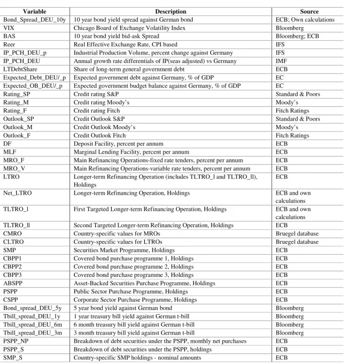
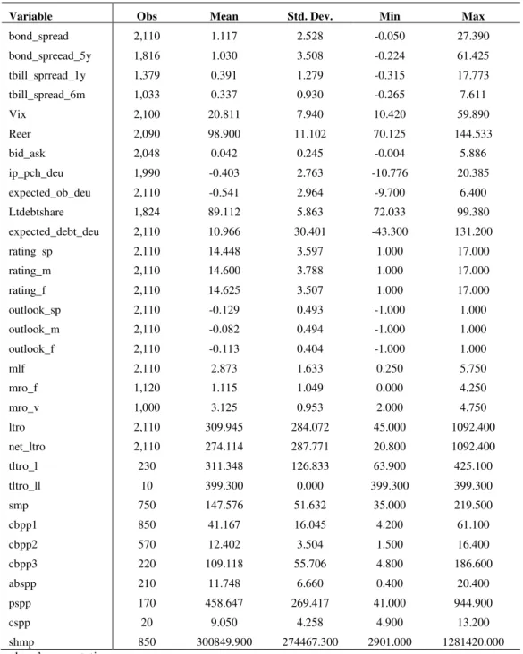
Table 1 presents the summary statistics for the relevant variables while data definitions and sources are explained in more detail in the Appendix.
[Table 1]
4.2 The Quantitative Easing Data
One of the main purposes of the paper is to check the potential effects of the ECB interventions on government bond yield spreads in the euro area. Therefore, we have collected data related to the ECB intervention through various strands of QE. In practice, the ECB classifies its policy measures as standard and non-standard measures. The description of these measures is detailed in below.
4.2.1 Standard measures
The open market operations of the Eurosystem consist of the main refinancing operations (MROs) and longer-term refinancing operations (LTROs). MROs are set by the governing council of the ECB and provides a bulk of liquidity to the banking system. We denoted the main refinancing operations fixed rate by MRO_F. It is obtained from the ECB and is available from 1 January 1999 until 16 March 2016, except for the period from 28 June 2000 to 15 October 2008. In this period the ECB set the main refinancing operations variable rate which we denoted by MRO_V. The interest rate levels are in percentage per annum.
CMRO is the monthly country-specific values for the MROs, these values are in Euro millions, data is obtained from the Bruegel database and it is available from January 2003. Two core countries, France and the Netherlands are not covered.
16
LTROs provide additional longer-term refinancing to the financial sector. We denoted the holdings of the Longer-term Refinancing Operations by LTRO, it includes LTROs, TLTRO_I and TLTRO_II. It is collected from the weekly financial statement of the ECB using the values at the end of each month. These values are in Euro billions. Net-LTRO is the accumulated values of the LTRO that excludes TLTROs (Net_LTRO = LTRO – TLTRO_I – TLTRO_II). From September 1, 2014 the accumulated values are based on our calculations using the values reported by the ECB in the weekly financial statement.
CLTRO is the monthly country-specific values for the LTROs, these values are in Euro millions. Data is obtained from the Bruegel database and it is available from January 2003. Two countries, France and the Netherlands are not covered.
4.2.2 Non-standard measures
The targeted longer term refinancing operations (TLTROs) provide financing to credit institutions for periods of up to four years. The accumulated amounts of the first series of the targeted longer term refinancing operations which we denoted by TLTRO_I are based on our own calculations using the reported settled values in the weekly financial statement of the ECB. The second series of the targeted longer-term refinancing operations started in June 2016 and is denoted by TLTRO_II. Data is available from July 2016 and it is collected from the weekly financial statement of the ECB.
The expanded asset purchase programme (APP) includes all the purchase programmes under which private and public sector securities are purchased to address the risks of a too prolonged period of low inflation. This programme consists of three terminated and four ongoing purchase programmes.
17
Securities Market Programme (SMP) was started on 10May 2010 and was terminated on
6 September 2012. The existing securities will be held to maturity. Daily data is available from 17 May 2010 on the ECB database. Here we used the SMP holdings at the end of each month. These values are in Euro billions. Variable SMP_S is the country specific nominal holdings under SMP. Values are reported for the peripheral countries (Italy, Greece, Ireland, Portugal and Spain) at the end of each year and are in Euro billions.
Covered Bond Purchase Programme (denoted by CBPP1) started on 2 July 2009 and terminated on 30 June 2010 when it reached a nominal amount of €60 billion. The assets bought
under this programme will be held to maturity. Daily data is available from the 9July 2009. We
used the holdings at the end of each month. These values are in Euro billions.
Covered bond Purchase Programme 2 (CBPP2) started on November 2011 and ended on 31 December 2012 when it reached the amount of €16.4 billion. The assets bought under this programme will be held to maturity. Daily data is available from 11 November 2011, we used the holdings at the end of each month. These values are in Euro billions.
4.2.2.2 Ongoing programmes
Covered Bond Purchase Programme 3 (CBPP3) started on 20 October 2014. As ECB mentions, this measure “helps to enhance the functioning of the monetary policy transmission mechanism, supports financing conditions in the euro area, facilitates credit provision to the real economy and generates positive spillovers to other markets”. Daily data is available from 24 October 2014. We used the holdings at the end of each month. The values are in Euro billions.
Asset-Backed Securities Purchase Programme (ABSPP) started on 21 November 2014. Daily data is available from 28 November 2014. We used the holdings at the end of each month. These values are in Euro billions.
18
Public Sector Purchase Programme (PSPP) started on March 2015. Daily data is available from 13 March 2015. We used the holdings at the end of each month. These values are in Euro billions. PSPP_N is the country-specific monthly net purchases under PSPP. Monthly data is available on the ECB and it covers all the sample countries except Greece. The values are in Euro millions. Variable PSPP_S is the country-specific PSPP holdings at the end of the sample period. It covers all the sample countries except Greece. Values are in Euro millions.
Corporate Sector Purchase Programme (CSPP) started on 8 June 2016. Daily data is available from 10 June 2016. We used the holdings at the end of each month. These values are in Euro billions.
5. Empirical Results
5.1. Selection of key yield spread determinants
In order to be able to estimate a so-called baseline specification, we first report the results of the Bayesian Model Averaging (BMA) and of the Weighted-Average Least Squares (WALS) procedures to select the core variables. Results are displayed in Tables 2.a-2c, which are organized in a similar way. First, we show the output of BMA, which provides information about estimated coefficients, their t-ratios and posterior inclusion probabilities - PIP (the posterior probability that a variable is included in the model – ranging from zero to one). Then, our validation of the estimation results using the WALS instead is carried out by implementing the original procedure without any preliminary scaling of focus and auxiliary regressors. While the output of WALS is similar to that of BMA, the main difference is that former does not allow for computing the posterior inclusion probabilities. Estimation results for the focus and the auxiliary parameters are displayed in the upper and the lower panels of each table. We run two alternative setups for
19
robustness purposes. Setup 1 considers the expected overall balance (relative to Germany), long-term debt share and expected public debt (relative to Germany) as part of the focus regressors. Setup 2 considers those three variables as auxiliary regressors, leaving only the constant term as the focus regressor.
We can draw some initial conclusions. Starting with Table 2a, we observe that the fiscal variables appear consistently as key determinants of the yield spreads. As expected, higher (lower) differences of the expected debt (budget balance) vis-à-vis the expected respective variables for Germany, increase (decrease) the sovereign yield spreads (Table 2a). Moreover, liquidity and risk factors, proxied respectively by the bid-ask spread and by the VIX indicator are also responsible for the upward movements in the yield spreads.
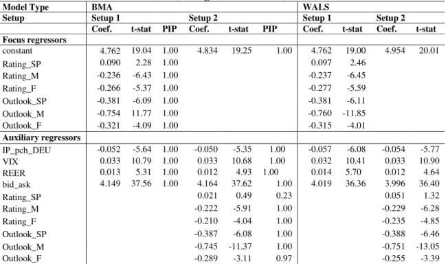
In addition, looking at Table 2.b, the improvement of sovereign rating notations and outlook conditions contribute to decrease the yield spreads. This initial result is in line with our a priori conjecture and with the existing results in the literature, as discussed in Section 2.
In terms of the so-called non-conventional monetary policy measures, our first indication points to the relevance of the holdings at the end of the month in the SMP in reducing the yield spreads (Table 2c). We have used the QE variables in levels in both the BMA and WALS exercises. Overall, the output of BMA is similar to that of WALS, which is reassuring. Next, we run our main panel regressions.
[Tables 2a, b, c]
5.2. Panel analysis
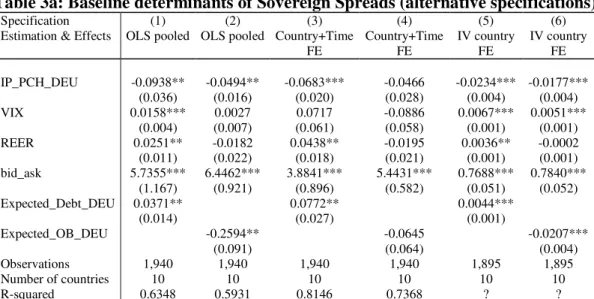
For the baseline specification, we used industrial production indices in terms of their differences vis-à-vis Germany, fiscal policy variables differences towards Germany as well, and liquidity, international risk, real effective exchange rate data. In Table 3a, we can confirm for the
20
10 Euro area economies in our sample that all variables, when statistically significant, have the expected effect on the yield spreads, in line with previous studies.
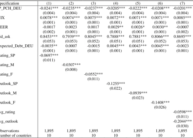
Furthermore, better ratings and outlooks (irrespectively of the agency) also decrease the sovereign yield spreads (Table 3b).
[Tables 3a and 3b]
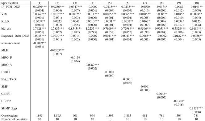
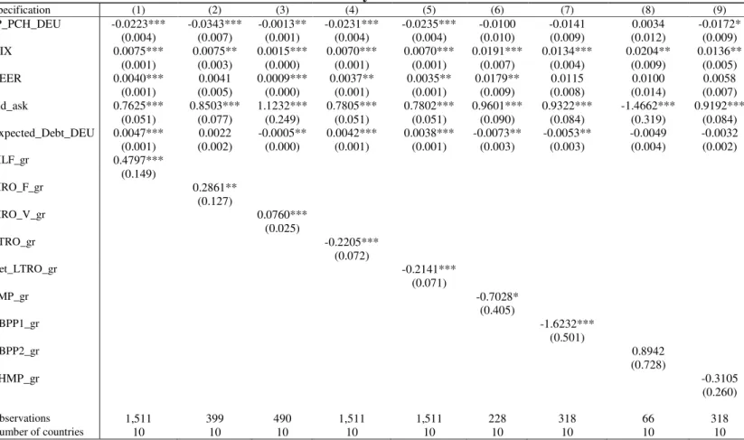
Turning to some of the non-conventional measures of the ECB, we can conclude from Tables 4a, 4b (notably when using growth rates), that these interventions (although not all measures are statistically significant) contributed to reduce the average euro area sovereign yield spreads, which was, to some extent, an objective of such measures.
[Table 4a, 4b]
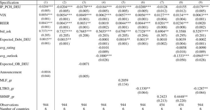
Our results are robust to several sensitivity exercises and robustness checks. First, we looked more closely at the impact of the Global Financial Crisis by splitting the baseline regressions into before and after (2009:01). In Table 5, we see that, for instance, the market pricing of sovereign ratings and outlooks is essentially done after the crisis, being less relevant before that period. In addition, a measure such as the LTRO, aimed at liquidity-providing long-term refinancing operations, only contributes to the reduction of yield spreads after the crisis.
Another important evidence of the relevance of crisis is the fact that the international risk factor, the VIX, is price around 7 to 8 times more after the crisis. In the same vein, the level of liquidity also becomes a key determinant after the crisis, being either essentially not statistically significant before or priced at a lower magnitude.
[Table 5]
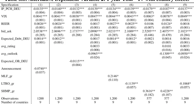
Second, we replaced our main dependent variable for the yield spreads by other maturities of government bond spreads (5-years) or T-bill spreads (12 and 6 months) – alternative dependent variable 1, 2 and 3, respectively. In fact, some of the non-conventional measures of the ECB may
21
have had an effect on the intermediate bond maturities as well. Our results displayed in Tables 6a, 6b, 6c, show that most notably for the one year and 6-month maturities the LTRO reduced those sovereign spreads.
On the other hand, we see that while rating notations are statistically significant for the 5-year yield spreads, rating outlooks become more relevant for the shorter bonds’ maturities (1 5-year and 6 months). Finally, the other baseline yield spread determinants keep their relevance for these shorter maturities as well. 5
[Tables 6.a, 6.b and 6.c]
5.3. Time-Varying Coefficients Model
We estimated the Time-Varying Coefficients (TVC) models for a set of relevant core determinants. Figure 1 illustrates the time varying characteristics of several determinants of the sovereign yield spreads.
[Figure 1]
For instance, we can observe that in the interquartile charts, increases in the VIX indicator have an upward effect on the sovereign yield spreads, but the magnitude of the effect changes through time. In fact, that effect rises during the 2010-2012 period, and then becomes more mitigated as the economic and financial crisis tends to be less acute, notably after 2013. A somewhat similar result is present in terms of the bid-ask spread, where liquidity issues where more prominent in terms of the size of the effect in the period 2010-2014. In addition, the impact
5 We also assessed the relevance of the announcement dates of the QE-measures, notably since for some cases, such
as the case of the OMT, there were no securities bought at all. The results were not too robust overall, although some evidence is captured for the OMT announcement date (2 August 2012).
22
on yield spreads stemming from the REER also spikes up in the period 2011-2012, with a real exchange rate appreciation increase the spreads. Regarding the economic conditions, this determinant of the yields spreads is clearly more relevant and more heavily priced in the markets in the period 2009-2013, when the crisis hit the euro area harder.
Focussing on the country specific results, we report in Figures 2 to 11, the TVC of the estimations for the expected government debt difference vis-à-vis Germany, the average ratings of the three main rating agencies, and two measures of monetary policy, CBPP1 and LTRO.
[Figures 2-11]
From those sets of TVC country specific results, we can draw several conclusions. The increase in the expected government debt ratio, versus the German one, is more strongly relevant as an upward determinant of yield spreads in the crisis period, peaking in 2012. This is true for all the euro area countries in our sample except in the cases of Austria and Finland (sovereigns that actually maintained a stronger rating in that period).
Considering now the market pricing of the sovereign ratings, we observe an increase in the effect on yield spreads in the period 2011-2012, when several downgrades occurred for most countries.
Turning to the QE measures, the CBPP1 non-standard measure has contributed to bring down sovereign yield spreads in all euro area countries in the analysis. Moreover, that downward effect has been very pronounced particularly in the crisis period, 2011-2013. In addition, and if we look at an example of a more standard measure, the LTRO, we can conclude that this measure also contributed to reduce yield spreads in most countries as well.
23
6. Conclusion
We have assessed the determinants of sovereign bond yield spreads in the period 1999:01-2016:07, taking into account the so-called non-conventional monetary policy measures in the euro area. Such QE measures implemented by the ECB might have had an effect on country specific Euro area yield spreads.
Regarding the so-called Quantitative Easing measures, purchases on behalf of the ECB of national government bonds, we have considered Covered Bond Purchase Programmes (CBPP), Securities Market Programme (SMP), Asset-Backed Securities Purchase Programme (ABSPP), Public Sector Purchase Programme (PSPP), and Corporate Sector Purchase Programme (CSPP).
From a methodological point of view, we have implemented a two-step approach. First, we have confirmed, by means of model selection methods, and estimated (by means of panel analysis) the determinants of sovereign bond yield spreads. Second, we have computed bivariate time-varying coefficient models of each determinant on government bond yield spreads and analysed the temporal dynamics of the resulting estimates for such coefficients.
The main results are as follows. i) Industrial production (difference vis-à-vis Germany), fiscal policy variables differences towards Germany as well, and liquidity, international risk, real effective exchange rate data when statistically significant, have the expected effect on the yield spreads. ii) Better ratings and outlooks, from all three main rating agencies also decrease the sovereign yield spreads. iii) Some non-conventional measures of the ECB contributed to reduce the average euro area sovereign yield spreads. iv) Market pricing of sovereign ratings and outlooks is essentially done after the crisis v) the international risk factor (VIX) is price around 7 to 8 times more after the crisis. vi) Liquidity is also a key determinant after the crisis.
24
Regarding the second step we find that: viii) the Time-Varying Coefficients models shows the VIX effect having a higher magnitude through the period 2010-2012. ix) Liquidity issues where more prominent in terms of the size of the effect in the period 2010-2014. x) The impact on yield spreads stemming from the REER also spikes up in the period 2011-2012. xi) Industrial production is more heavily priced in the markets in the period 2009-2013. xii) The increase in the expected government debt ratio, versus the German one, peaks in 2012 for all the euro area countries except in the cases of Austria and Finland. xiii) Market pricing of the sovereign ratings increased in period 2011-2012. xiv) The CBPP1 contributed to bring down sovereign yield spreads in all euro area countries particularly in the period 2011-2013. xv) The LTRO contributed to reduce yield spreads in most countries as well.
From a policy perspective, it is unclear for how long the ECB will continue to implement its QE measures, which might be seen as a risk for the more fiscally and financially vulnerable euro area economies.
25
References
1. Acharya, V., Drechsler, I., & Schnabl, P. (2014). A pyrrhic victory? Bank bailouts and sovereign credit risk. Journal of Finance, 69 (6), 2689-2739.
2. Afonso, A., Arghyrou, M., Bagdatoglou, G., & Kontonikas, A. (2015). “On the time-varying
relationship between EMU sovereign spreads and their determinants”. Economic Modelling,
44, 363-371.
3. Afonso, A., Arghyrou, M., & Kontonikas, A. (2014). “Pricing sovereign bond risk in the European Monetary Union area: an empirical investigation”. International Journal of Finance
& Economics, 19 (1), 49-56.
4. Afonso, A., Furceri, D., & Gomes, P. (2012). “Sovereign credit ratings and financial markets
linkages: application to European data”, Journal of International Money and Finance, 31 (3), 606-638.
5. Afonso, A., & Jalles, J. T. (2016). “Economic Volatility and Sovereign Yields' Determinants:
A Time-Varying Approach”. ISEG Economics Department WP 04/2016/DE/UECE.
6. Afonso, A., & Martins, M. M. (2012). Level, slope, curvature of the sovereign yield curve, and
fiscal behaviour. Journal of Banking & Finance, 36(6), 1789-1807.
7. Afonso, A., & Rault, C. (2015). “Short and Long-run Behaviour of Long-term Sovereign Bond
Yields”, Applied Economics, 47 (37), 3971-3993.”,
8. Akitoby B, & Stratmann T (2008). “Fiscal policy and financial markets”. Economic Journal,
118, 1971-1985.
9. Alesina, A., De Broeck, M., Prati, A., & Tabellini, G. (1992). Default risk on government debt
26
10. Aghion, P., & Marinescu, I. (2008). Cyclical Budgetary Policy and Economic Growth:
What Do We Learn from OECD Panel Data?. NBER Macroeconomics annual 2007, 22, 251-297.
11. Aizenman, J., Hutchison, M., & Jinjarak, Y. (2013). What is the risk of European sovereign
debt defaults? Fiscal space, CDS spreads and market pricing of risk. Journal of International
Money and Finance, 34, 37-59.
12. Arghyrou, M. G., & Kontonikas, A. (2012). The EMU sovereign-debt crisis:
Fundamentals, expectations and contagion. Journal of International Financial Markets,
Institutions and Money, 22(4), 658-677.
13. Arghyrou, M. G., & Tsoukalas, J. D. (2011). The Greek debt crisis: Likely causes,
mechanics and outcomes. The World Economy, 34(2), 173-191.
14. Aßmann, C., & Boysen-Hogrefe, J. (2012). “Determinants of government bond spreads in
the euro area: in good times as in bad”. Empirica, 39 (3), 341-356.
15. Barrios, S., Iversen, P., Lewandowska, M., & Setzer, R. (2009). Determinants of intra-euro
area government bond spreads during the financial crisis (No. 388). Directorate General Economic and Financial Affairs (DG ECFIN), European Commission.
16. Bernoth, K., & Erdogan, B. (2012). “Sovereign bond yield spreads: A time-varying
coefficient approach”. Journal of International Money and Finance, 31 (3), 639-656.
17. Boysen-Hogrefe, J. (2013). “A dynamic factor model with time-varying loadings for euro
area bond markets during the debt crisis”. Economics Letters, 118 (1), 50-54.
18. Caggiano, G., & Greco, L. (2012). Fiscal and financial determinants of Eurozone sovereign
27
19. Costantini, M., Fragetta, M. & Melina, G. (2014). “Determinants of sovereign bond yield
spreads in the EMU: An optimal currency area perspective”. European Economic Review, 70, 337-349.
20. D’Agostino, A., & Ehrmann, M. (2014). “The pricing of G7 sovereign bond spreads–The
times, they are A-changing”. Journal of Banking and Finance, 47, 155-176.
21. Delatte, A., Fouquau, J. & Portes, R. (2014). “Regime-Dependent Sovereign Risk Pricing
during the Euro Crisis”. ESRB Working Paper, No.9.
22. De Santis, R.A., (2012). The euro area sovereign debt crisis: save haven, credit rating
agencies and the spread of the fever from Greece, Ireland and Portugal. ECB Working Paper
1419.
23. Di Cesare, A., G. Grande, M. Manna, & M. Taboga (2012), “Recent Estimates of Sovereign
Risk Premia for Euro-Area Countries”. Questioni di Economia e Finanza Occasional Papers. Bank of Italy, Economic Research and International Relations Area.
24. Easterly, W., & Rebelo, S. (1993). Fiscal policy and economic growth. Journal of monetary
economics, 32(3), 417-458.
25. Einmahl, J. H., Kumar, K., & Magnus, J. R. (2011). On the choice of prior in Bayesian
model averaging. CentER Working Paper No. 2011-003.
26. Elmendorf, D. W., & Mankiw, N. G. (1999). Government debt. Handbook of
macroeconomics, 1, 1615-1669.
27. Favero, C., Pagano, M., & Von Thadden, E. (2010). How Does Liquidity Affect
Government Bond Yields? Journal of Financial and Quantitative Analysis, 45(1), 107-134.
28. Fawley, B., Neely, C. (2013). “Four stories of quantitative easing”. Federal Reserve Bank
28
29. Gajewski, P. (2014). “Sovereign spreads and financial market behavior before and during
the crisis”. Lodz Economics Working Papers, 4/2014. University of Lodz, Faculty of Economics and Sociology
30. Georgoutsos, D., & Migiakis, P. (2013). “Heterogeneity of the determinants of euro-area
sovereign bond spreads; what does it tell us about financial stability?” Journal of Banking and
Finance, 37 (11), 4650-4664.
31. Gerlach, S., Schulz, A., & Wolff, G.B. (2010). Banking and sovereign risk in the euro area.
CEPR Discussion Paper No. 7833.
32. Gómez-Puig, M., Sosvilla-Rivero, S. & Ramos-Herrera, M.C. (2014). “An update on EMU
sovereign yield spread drivers in times of crisis: A panel data analysis”. North American
Journal of Economics and Finance, 30, 133-153.
33. Joyce, M., Lasaosa, A., Stevens, I., Tong, M. (2011). “The financial market impact of
quantitative easing in the United Kingdom”. International Journal of Central Banking, 7(3), 113-161.
34. Krishnamurthy, A., Vissing-Jorgensen, A. (2011). “The effects of quantitative easing on
interest rates: channels and implications for policy”. NBER WP 17555.
35. Klose, J. & Weigert, B. (2014). “Sovereign Yield Spreads During the Euro Crisis:
Fundamental Factors Versus Redenomination Risk”, International Finance, 17(1), 25-50.
36. Magnus, J. R., Powell, O., & Prüfer, P. (2010). A comparison of two model averaging
techniques with an application to growth empirics. Journal of econometrics, 154(2), 139-153.
37. Malik, A., & Temple, J. R. (2009). The geography of output volatility. Journal of
29
38. Manganelli, S., & Wolswijk, G. (2009). What drives spreads in the euro area government
bond market?. Economic Policy, 24(58), 191-240.
39. Mody, A. (2009). From Bear Stearns to Anglo Irish: how eurozone sovereign spreads
related to financial sector vulnerability. International Monetary Fund Working Paper 09/108.
40. Paniagua, J., Sapena, J., & Tamarit, C. (2016). “Sovereign debt spreads in EMU: The
time-varying role of fundamentals and market distrust”. Journal of Financial Stability.
41. Pozzi, L., & Sadaba, B. (2015). “Detecting regime shifts in euro area government bond risk
pricing: the impact of the financial crisis”. Mimeo.
42. Raftery, A. E. (1995). Bayesian model selection in social research. Sociological
methodology, 111-163.
43. Sala-i-Martin, X., Doppelhofer, G., & Miller, R.I. (2004). Determinants of long-term
growth: a Bayesian averaging of classical estimates (BACE). American Economic Review,
94(4), 813-835.
44. Schuknecht, L., J. von Hagen & G. Wolswijk (2009). "Government Risk Premiums in the
Bond Market: EMU and Canada", European Journal of Political Economy, 25, 371-384.
45. Schlicht, E. (1985). Isolation and Aggregation in Economics, Berlin-Heidelberg- New
York- Tokyo: Springer-Verlag.
46. Schlicht, E. (1988). Variance Estimation in a Random Coefficients Model. Paper presented
at the Econometric Society European Meeting Munich 1989.
47. Silvapulle, P., Fenech, J., Thomas, A. & Brooks, R. (2016). “Determinants of sovereign
bond yield spreads and contagion in the peripheral EU countries”. Economic Modelling, 58, 83-92.
30
APPENDIX
Table A1. Data Description and Sources
Variable Description Source
Bond_Spread_DEU_10y 10 year bond yield spread against German bond ECB; Own calculations VIX Chicago Board of Exchange Volatility Index Bloomberg
BAS 10 year bond yield bid-ask Spread Bloomberg; ECB Reer Real Effective Exchange Rate, CPI based IFS
IP_PCH_DEU_p Industrial Production Volume, percent change against Germany IFS IP_PCH_DEU Annual growth rate differentials of IP(seas adjusted) vs Germany IMF LTDebtShare Share of long-term general government debt ECB Expected_Debt_DEU/_p Expected government debt against Germany, % of GDP EC Expected_OB_DEU/_p Expected government budget balance against Germany, % of GDP EC
Rating_SP Credit rating S&P Standard & Poors
Rating_M Credit rating Moody’s Moody’s
Rating_F Credit rating Fitch Fitch Ratings
Outlook_SP Credit Outlook S&P Standard & Poors
Outlook_M Credit Outlook Moody’s Moody’s
Outlook_F Credit Outlook Fitch Fitch Ratings DF Deposit Facility, percent per annum ECB MLF Marginal Lending Facility, percent per annum ECB MRO_F Main Refinancing Operations-fixed rate tenders, percent per annum ECB MRO_V Main Refinancing Operations-variable rate tenders, percent per annum ECB LTRO Longer-term Refinancing Operation (includes TLTRO_l and TLTRO_ll),
Holdings
ECB
Net_LTRO Longer-term Refinancing Operation, Holdings ECB and own calculations TLTRO_l First Targeted Longer-term Refinancing Operation, Holdings ECB and own
calculations TLTRO_ll Second Targeted Longer-term Refinancing Operation, Holdings ECB
CMRO Country-specific values for MROs Bruegel database CLTRO Country-specific values for LTROs Bruegel database SMP Securities Market Programme, Holdings ECB
CBPP1 Covered bond purchase programme 1, Holdings ECB CBPP2 Covered bond purchase programme 2, Holdings ECB CBPP3 Covered bond purchase programme 3, Holdings ECB ABSPP Asset-Backed Securities Purchase Programme, Holdings ECB PSPP Public Sector Purchase Programme, Holdings ECB CSPP Corporate Sector Purchase Programme, Holdings ECB Bond_spread_DEU_5y 5 year bond yield against German bond Bloomberg Tbill_spread_DEU_1y 1 year treasury bill yield against German t-bill Bloomberg Tbill_spread_DEU_6m 6 month treasury bill yield against German t-bill Bloomberg Tbill_spread_DEU_3m 3 month treasury bill yield against German t-bill Bloomberg PSPP_NP Breakdown of debt securities under the PSPP, monthly net purchases ECB PSPP_S Breakdown of debt securities under the PSPP, holdings ECB SMP_S Country-specific SMP holdings - nominal amounts ECB
Notes: Expected budget balances and government debt are the differences vis-à-vis Germany of the European Commission vintage forecasts, taking the same value in the months between each forecast vintage. The volumes securities purchases are for the overall euro area.
31
Table 1. Summary Statistics
Variable Obs Mean Std. Dev. Min Max
bond_spread 2,110 1.117 2.528 -0.050 27.390 bond_spreead_5y 1,816 1.030 3.508 -0.224 61.425 tbill_sprread_1y 1,379 0.391 1.279 -0.315 17.773 tbill_spread_6m 1,033 0.337 0.930 -0.265 7.611 Vix 2,100 20.811 7.940 10.420 59.890 Reer 2,090 98.900 11.102 70.125 144.533 bid_ask 2,048 0.042 0.245 -0.004 5.886 ip_pch_deu 1,990 -0.403 2.763 -10.776 20.385 expected_ob_deu 2,110 -0.541 2.964 -9.700 6.400 Ltdebtshare 1,824 89.112 5.863 72.033 99.380 expected_debt_deu 2,110 10.966 30.401 -43.300 131.200 rating_sp 2,110 14.448 3.597 1.000 17.000 rating_m 2,110 14.600 3.788 1.000 17.000 rating_f 2,110 14.625 3.507 1.000 17.000 outlook_sp 2,110 -0.129 0.493 -1.000 1.000 outlook_m 2,110 -0.082 0.494 -1.000 1.000 outlook_f 2,110 -0.113 0.404 -1.000 1.000 mlf 2,110 2.873 1.633 0.250 5.750 mro_f 1,120 1.115 1.049 0.000 4.250 mro_v 1,000 3.125 0.953 2.000 4.750 ltro 2,110 309.945 284.072 45.000 1092.400 net_ltro 2,110 274.114 287.771 20.800 1092.400 tltro_l 230 311.348 126.833 63.900 425.100 tltro_ll 10 399.300 0.000 399.300 399.300 smp 750 147.576 51.632 35.000 219.500 cbpp1 850 41.167 16.045 4.200 61.100 cbpp2 570 12.402 3.504 1.500 16.400 cbpp3 220 109.118 55.706 4.800 186.600 abspp 210 11.748 6.660 0.400 20.400 pspp 170 458.647 269.417 41.000 944.900 cspp 20 9.050 4.258 4.900 13.200 shmp 850 300849.900 274467.300 2901.000 1281420.000
32
Table 2.a Bayesian Model Averaging and Weighted-Average Least Squares (economic and fiscal fundamentals)
Model Type BMA WALS
Setup Setup 1 Setup 2 Setup 1 Setup 2
Coef. t-stat PIP Coef. t-stat PIP Coef. t-stat Coef. t-stat Focus regressors constant -2.138 -2.83 1.00 -2.000 -2.16 1.00 -3.499 -4.09 -3.482 -4.09 Expected_OB_DEU -0.176 -10.89 1.00 -0.175 -10.77 Ltdebtshare 0.025 3.61 1.00 0.027 4.02 Expected_debt_DEU 0.026 17.03 1.00 0.028 17.04 Auxiliary regressors IP_pch_DEU -0.090 -4.73 1.00 -0.089 1.44 0.74 -0.091 -4.92 -0.083 -4.61 VIX 0.012 1.52 0.77 0.011 1.44 0.74 0.018 3.67 0.013 2.90 REER 0.001 0.26 0.09 0.001 0.26 0.09 0.012 1.98 0.007 1.34 bid_ask 5.498 35.97 1.00 5.501 35.90 1.00 5.285 34.70 5.304 35.01 Expected_OB_DEU -0.175 -10.77 1.00 -0.181 -11.42 Ltdebtshare 0.023 2.66 0.94 0.032 4.79 Expected_debt_DEU 0.026 16.93 1.00 0.026 16.48
Note: BMA stands for Bayesian Model Averaging; WALS stands for Weighted Average Least Squares. BMA’s output includes coefficient estimates, their t-statistics and the PIP (probability of inclusion). WALS’ output includes coefficient estimates and their t-statistics. Setup 1 considers the expected overall balance (relative to Germany), long-term debt share and expected public debt (relative to Germany) as part of the focus regressors. Setup 2 considers those three variables as auxiliary regressors, leaving only the constant term as the focus regressor. Refer to the main text for further details.
Table 2.b Bayesian Model Averaging and Weighted-Average Least Squares (ratings and outlooks)
Model Type BMA WALS
Setup Setup 1 Setup 2 Setup 1 Setup 2
Coef. t-stat PIP Coef. t-stat PIP Coef. t-stat Coef. t-stat Focus regressors constant 4.762 19.04 1.00 4.834 19.25 1.00 4.762 19.00 4.954 20.01 Rating_SP 0.090 2.28 1.00 0.097 2.46 Rating_M -0.236 -6.43 1.00 -0.237 -6.45 Rating_F -0.266 -5.37 1.00 -0.277 -5.59 Outlook_SP -0.381 -6.09 1.00 -0.381 -6.11 Outlook_M -0.754 11.77 1.00 -0.760 -11.85 Outlook_F -0.321 -4.09 1.00 -0.315 -4.01 Auxiliary regressors IP_pch_DEU -0.052 -5.64 1.00 -0.050 -5.35 1.00 -0.057 -6.08 -0.054 -5.77 VIX 0.033 10.79 1.00 0.033 10.68 1.00 0.032 10.41 0.033 10.90 REER 0.013 5.31 1.00 0.012 4.93 1.00 0.014 5.70 0.012 4.64 bid_ask 4.149 37.56 1.00 4.164 37.62 1.00 4.019 36.36 3.996 36.40 Rating_SP 0.021 0.49 0.23 0.051 1.32 Rating_M -0.222 -5.91 1.00 -0.229 -6.28 Rating_F -0.210 -4.04 1.00 -0.235 -4.85 Outlook_SP -0.387 -6.08 1.00 -0.388 -6.46 Outlook_M -0.745 -11.37 1.00 -0.751 -13.05 Outlook_F -0.289 -3.11 0.97 -0.255 -3.39
Note: BMA stands for Bayesian Model Averaging; WALS stands for Weighted Average Least Squares. BMA’s output includes coefficient estimates, their t-statistics and the PIP (probability of inclusion). WALS’ output includes coefficient estimates and their t-statistics. Setup 1 considers the expected overall balance (relative to Germany), long-term debt share and expected public debt (relative to Germany) as part of the focus regressors. Setup 2 considers those three variables as auxiliary regressors, leaving only the constant term as the focus regressor. Refer to the main text for further details.
33
Table 2.c Bayesian Model Averaging and Weighted-Average Least Squares (QE: refinancing operations and purchase programmes)
Model Type BMA WALS
Setup Setup 1 Setup 2 Setup 1 Setup 2
Coef. t-stat PIP Coef. t-stat PIP Coef. t-stat Coef. t-stat Focus regressors constant 30.265 5.99 1.00 27.03 11.36 1.00 30.25 6.03 28.087 6.50 MLF -0.887 -0.47 1.00 -1.407 -0.74 MRO_F 2.246 1.02 1.00 3.155 1.40 LTRO 0.001 1.78 1.00 0.001 1.85 CBPP1 0.021 0.59 1.00 0.023 0.64 SMP 0.002 0.94 1.00 0.002 0.82 SHMP (log) -0.252 -0.77 1.00 -0.209 -0.64 Auxiliary regressors IP_pch_DEU -0.205 -6.71 1.00 -0.200 -6.43 1.00 -0.197 -6.67 -0.191 -6.28 VIX -0.005 -0.36 0.15 -0.005 -0.36 0.15 -0.023 -1.20 -0.019 -1.12 REER -0.284 -15.99 1.00 -0.283 -15.7 1.00 -0.286 -17.24 -0.271 -15.39 bid_ask 5.39 24.00 1.00 5.421 24.30 1.00 5.157 24.50 5.261 23.88 MLF 0.371 0.60 0.32 -0.823 -0.52 MRO_F 0.386 0.49 0.26 2.349 1.25 LTRO 0.001 1.02 0.58 0.001 1.79 CBPP1 0.028 0.96 0.51 0.017 0.57 SMP 0.001 0.56 0.29 0.002 0.97 SHMP (log) -0.019 -0.17 0.09 -0.140 -0.52
Note: BMA stands for Bayesian Model Averaging; WALS stands for Weighted Average Least Squares. BMA’s output includes coefficient estimates, their t-statistics and the PIP (probability of inclusion). WALS’ output includes coefficient estimates and their t-statistics. Setup 1 considers the expected overall balance (relative to Germany), long-term debt share and expected public debt (relative to Germany) as part of the focus regressors. Setup 2 considers those three variables as auxiliary regressors, leaving only the constant term as the focus regressor. Refer to the main text for further details.
Table 3a: Baseline determinants of Sovereign Spreads (alternative specifications)
Specification (1) (2) (3) (4) (5) (6)
Estimation & Effects OLS pooled OLS pooled Country+Time FE Country+Time FE IV country FE IV country FE IP_PCH_DEU -0.0938** -0.0494** -0.0683*** -0.0466 -0.0234*** -0.0177*** (0.036) (0.016) (0.020) (0.028) (0.004) (0.004) VIX 0.0158*** 0.0027 0.0717 -0.0886 0.0067*** 0.0051*** (0.004) (0.007) (0.061) (0.058) (0.001) (0.001) REER 0.0251** -0.0182 0.0438** -0.0195 0.0036** -0.0002 (0.011) (0.022) (0.018) (0.021) (0.001) (0.001) bid_ask 5.7355*** 6.4462*** 3.8841*** 5.4431*** 0.7688*** 0.7840*** (1.167) (0.921) (0.896) (0.582) (0.051) (0.052) Expected_Debt_DEU 0.0371** 0.0772** 0.0044*** (0.014) (0.027) (0.001) Expected_OB_DEU -0.2594** -0.0645 -0.0207*** (0.091) (0.064) (0.004) Observations 1,940 1,940 1,940 1,940 1,895 1,895 Number of countries 10 10 10 10 10 10 R-squared 0.6348 0.5931 0.8146 0.7368 ? ?
Note: Dependent variable is the 10-year bond yield spread (relative to Germany). Estimations by OLS and IV as indicated in the second row. Robust standard errors clustered at the country level are in parenthesis below each coefficient estimate. When applicable country and time effects were estimated but omitted for reasons of parsimony. A constant term was also estimated but omitted. *, **, *** denote statistical significance at the 10, 5, and 1 percent level, respectively.
34
Table 3b: Ratings and Outlooks determinants - IV with country effects
Specification (1) (2) (3) (4) (5) (6) (7) IP_PCH_DEU -0.0241*** -0.0235*** -0.0237*** -0.0205*** -0.0222*** -0.0208*** -0.0201*** (0.004) (0.004) (0.004) (0.004) (0.004) (0.004) (0.004) VIX 0.0078*** 0.0074*** 0.0075*** 0.0072*** 0.0071*** 0.0071*** 0.0085*** (0.001) (0.001) (0.001) (0.001) (0.001) (0.001) (0.001) REER -0.0017 0.0023 0.0017 0.0029** 0.0026* 0.0030** -0.0007 (0.002) (0.001) (0.001) (0.001) (0.001) (0.001) (0.002) bid_ask 0.8453*** 0.7939*** 0.8045*** 0.7888*** 0.7881*** 0.8066*** 0.8695*** (0.053) (0.053) (0.052) (0.051) (0.051) (0.052) (0.053) Expected_Debt_DEU -0.0035** 0.0007 -0.0015 0.0045*** 0.0043*** 0.0045*** -0.0023 (0.001) (0.001) (0.001) (0.001) (0.001) (0.001) (0.001) Rating_SP -0.0697*** (0.011) Rating_M -0.0307*** (0.008) Rating_F -0.0552*** (0.011) Outlook_SP -0.1255*** (0.022) Outlook_M -0.0939*** (0.023) Outlook_F -0.1408*** (0.026) avg_rating -0.0598*** (0.011) avg_outlook -0.2044*** (0.030) Observations 1,895 1,895 1,895 1,895 1,895 1,895 1,895 Number of countries 10 10 10 10 10 10 10
Note: Dependent variable is the 10-year bond yield spread (relative to Germany). Estimations by Two Stage Least Squares with lags of the dependent variable and regressors used as instruments. Robust standard errors clustered at the country level are in parenthesis below each coefficient estimate. Country effects were estimated but omitted for reasons of parsimony. A constant term was also estimated but omitted. *, **, *** denote statistical significance at the 10, 5, and 1 percent level, respectively.
35
Table 4.a: Refinancing and purchase programme determinants (in levels) - IV with country effects Specification (1) (2) (3) (4) (5) (6) (7) (8) (9) (10) IP_PCH_DEU -0.0230*** -0.0236*** -0.0347*** -0.0009 -0.0235*** -0.0233*** -0.0090 -0.0174* 0.0087 -0.0191** (0.004) (0.004) (0.007) (0.001) (0.004) (0.004) (0.010) (0.009) (0.012) (0.009) VIX 0.0067*** 0.0073*** 0.0082** 0.0011*** 0.0065*** 0.0065*** 0.0105** 0.0085** 0.0185* 0.0098** (0.001) (0.001) (0.003) (0.000) (0.001) (0.001) (0.005) (0.004) (0.010) (0.004) REER 0.0037** 0.0023 0.0042 0.0010*** 0.0031** 0.0032** 0.0163* 0.0046 0.0334* 0.0125 (0.001) (0.002) (0.005) (0.000) (0.001) (0.001) (0.009) (0.007) (0.017) (0.008) bid_ask 0.7621*** 0.7837*** 0.8543*** 1.2235*** 0.7809*** 0.7798*** 0.9596*** 0.9051*** 0.5828*** 0.9189*** (0.051) (0.052) (0.077) (0.245) (0.052) (0.052) (0.090) (0.084) (0.206) (0.083) Expected_Debt_DEU 0.0045*** 0.0030*** 0.0014 -0.0002 0.0041*** 0.0043*** -0.0068** -0.0002 -0.0122*** -0.0056** (0.001) (0.001) (0.002) (0.000) (0.001) (0.001) (0.003) (0.003) (0.004) (0.003) announcement -0.1089** (0.051) MLF -0.0203*** (0.007) MRO_F -0.0139 (0.034) MRO_V 0.0089*** (0.002) LTRO 0.0001 (0.000) Net_LTRO 0.0001 (0.000) SMP -0.0001 (0.001) CBPP1 0.0043* (0.002) CBPP2 -0.0301* (0.016) SHMP (log) 0.1122*** (0.038) Observations 1895 1,895 901 944 1,895 1,895 681 781 504 781 Number of countries 10 10 10 10 10 10 10 10 10 10
Note: Dependent variable is the 10-year bond yield spread (relative to Germany). Estimations by Two Stage Least Squares with lags of the dependent variable and regressors used as instruments. Robust standard errors clustered at the country level are in parenthesis below each coefficient estimate. Country effects were estimated but omitted for reasons of parsimony. A constant term was also estimated but omitted. *, **, *** denote statistical significance at the 10, 5, and 1 percent level, respectively.
36
Table 4.b: Refinancing and purchase programme determinants (in growth rates) - IV with country effects Specification (1) (2) (3) (4) (5) (6) (7) (8) (9) IP_PCH_DEU -0.0223*** -0.0343*** -0.0013** -0.0231*** -0.0235*** -0.0100 -0.0141 0.0034 -0.0172* (0.004) (0.007) (0.001) (0.004) (0.004) (0.010) (0.009) (0.012) (0.009) VIX 0.0075*** 0.0075** 0.0015*** 0.0070*** 0.0070*** 0.0191*** 0.0134*** 0.0204** 0.0136** (0.001) (0.003) (0.000) (0.001) (0.001) (0.007) (0.004) (0.009) (0.005) REER 0.0040*** 0.0041 0.0009*** 0.0037** 0.0035** 0.0179** 0.0115 0.0100 0.0058 (0.001) (0.005) (0.000) (0.001) (0.001) (0.009) (0.008) (0.014) (0.007) bid_ask 0.7625*** 0.8503*** 1.1232*** 0.7805*** 0.7802*** 0.9601*** 0.9322*** -1.4662*** 0.9192*** (0.051) (0.077) (0.249) (0.051) (0.051) (0.090) (0.084) (0.319) (0.084) Expected_Debt_DEU 0.0047*** 0.0022 -0.0005** 0.0042*** 0.0038*** -0.0073** -0.0053** -0.0049 -0.0032 (0.001) (0.002) (0.000) (0.001) (0.001) (0.003) (0.003) (0.004) (0.002) MLF_gr 0.4797*** (0.149) MRO_F_gr 0.2861** (0.127) MRO_V_gr 0.0760*** (0.025) LTRO_gr -0.2205*** (0.072) Net_LTRO_gr -0.2141*** (0.071) SMP_gr -0.7028* (0.405) CBPP1_gr -1.6232*** (0.501) CBPP2_gr 0.8942 (0.728) SHMP_gr -0.3105 (0.260) Observations 1,511 399 490 1,511 1,511 228 318 66 318 Number of countries 10 10 10 10 10 10 10 10 10
Note: Dependent variable is the 10-year bond yield spread (relative to Germany). Estimations by Two Stage Least Squares with lags of the dependent variable and regressors used as instruments. Robust standard errors clustered at the country level are in parenthesis below each coefficient estimate. Country effects were estimated but omitted for reasons of parsimony. A constant term was also estimated but omitted. *, **, *** denote statistical significance at the 10, 5, and 1 percent level, respectively.