Obstacle detection and collision avoidance method based on optical systems

Engenharia

Obstacle Detection and Collision Avoidance

Method Based on Optical Systems

(Versão final após defesa)

Ana Beatriz Botelho da Silva

Dissertação para obtenção do Grau de Mestre em

Engenharia Aeronáutica

(ciclo de estudos integrado)

Orientador: Prof. Doutor Kouamana Bousson

Dedication

I dedicate this work to two special people who, although they are no longer present, continue to be the main foundations of my life, my biggest examples. My grandfather, Joaquim, who with his hard work and will to succeed in life taught me to pursue my dreams without ever losing sight of reality. And my grandmother, Hortensia, who showed me that patience and kindness are two virtues we should aspire to live by. Together, they guide me to be who I am. They showed me that there is no perfection in life just as there are no easy roads without obstacles. However, it is up to each of us to go beyond them.

Acknowledgements

Although this dissertation was mainly developed in Portugal, it started in another European country, more specifically, in Poland. Between these two countries is, approximately, a trip of two thousand and five hundred kilometres by plane, which takes around three and a half hours. So, I would like to begin by thanking a Polish professor who not only helped me decide on the subject of my dissertation but was also by my side during the first steps, professor Paweł Rzucidłofrom Rzeszow University of Technology.

I would also like to thank all the professors of the department of Aerospace Sciences, who taught and guided me during these five years in Aeronautical Engineering. Especially professor Kouamana Bousson who agreed to be my supervisor and helped me overcome all the difficulties and new challenges.

To those friends, who I've known since childhood, thank you for the friendship that even with the distance was never lost. As for my classmates, thank you for all the moments that have become good memories.

To a special person from Terceira, who know me since I was born and was always available to help.

To my best friend and companion, thank you for your patience, company and help during this last journey.

In terms of family, I would start by thanking my sister and brother-in-law for always being by my side in this and all the journeys of my life, especially to my sister, who was there for me through good and bad moments since I was a small child who barely knew how to walk but dreamed of flying. To the most important people in my life, my parents, thank you for your patience, for listening to me, for teaching me and for encouraging me to fight for my dreams.

Abstract

The development of a new collision avoidance method, which can detect and calculate the necessary changes to prevent imminent accident, is the focal interest of this work. In aviation, the risk of collision is a delicate and important subject, which merits the right approach. With the continuing growth of air traffic and the introduction of RPASs (Remotely Piloted Aircraft System), it is necessary to find better solutions and develop new systems to keep the control of the airspace. In this work, the main objective is to obtain a complete and functional computational algorithm, which could be included in an obstacle detection and avoidance system. Its unique feature of optical detection makes it mostly appropriated for RPASs. The application of Optical Techniques is mostly used in aircrafts to detect objects under them [1] or even to prevent a collision with terrain [2]. Some technologies also use optic flow sensors to detect and prevent collisions [3, 4]. In this case, the optical system will be used to detect obstacles in front of the aircraft.

The detection of an obstacle will be performed by the two infrared cameras strategically positioned in the aircraft. The objectives to accomplish with this method are: capable of dealing with collision detection characteristics; in case of detecting a possible threat of collision, describing the safe zone as the area outside a conflict cone; assessing if the threat of collision previously detected is real; in case the danger is real, changing the aircraft’s trajectory by altering one or more flight characteristics. To achieve the most efficient method possible some theoretical methods were explored, like the Convex Hull Method, which is a simple geometrical method, and a variation method based on differential equations.

With the aim of testing the algorithm in different situations, a total of six possible cases were generated. All the results showed coherence and efficiency, which confirms the success of this computational algorithm as a detection and collision avoidance method.

Keywords

Aeronautic, Air Traffic, Collision Avoidance System, Optical Detection, Computational Algorithm

Resumo

O desenvolvimento de um novo sistema de prevenção de colisões, que consiga detetar e calcular as mudanças necessárias para prevenir um acidente iminente, é o interesse focal deste trabalho. Na aviação, o risco de colisão é um assunto delicado e importante, o qual merece a correta abordagem. Com o crescimento continuo do trafego aéreo e a introdução dos RPASs (Remotely Piloted Aircraft System), é necessário procurar melhores soluções e desenvolver novos sistemas para manter o controlo do espaço aéreo. Neste trabalho, o principal objetivo é obter um algoritmo computacional completo e funcional, o qual poderá ser incluído num sistema de deteção e evasão de obstáculos. A sua característica única de deteção ótica torna--o principalmente apropriado para RPASs.

A aplicação de Técnicas Óticas é principalmente utilizada nas aeronaves para deteção de objetos debaixo destas [1] ou mesmo para prevenir uma colisão com o terreno [2]. Algumas tecnologias utilizam sensores de fluxo ótico para detetar e prevenir colisões [3, 4]. Neste caso, o sistema ótico será utilizado para detetar obstáculos à frente da aeronave.

Os objetivos a realizar com este sistema são: capaz de lidar com as características de deteção de colisão; em caso de detetar uma possível ameaça de colisão, descrever a zona segura como a área fora do cone de conflito; avaliar se a ameaça de colisão é real; no caso do perigo ser real, mudar a trajetória da aeronave alterando uma ou mais característica de voo. Para obter o sistema mais eficiente possível alguns métodos teóricos foram explorados, como o método do ‘Convex Hull’, o qual é um simples método geométrico, e um método de variação com base nas equações diferenciais.

Com o objetivo de testar o sistema em diferentes situações, um total de seis casos possíveis foram gerados. Todos os resultados mostraram coerência e eficácia, o que confirma o sucesso do algoritmo computacional como um sistema de deteção e evasão de colisões.

Palavras-chave

Aeronáutica, Trafego Aéreo, Sistema de Prevenção de Colisões, Deteção Ótica, Algoritmo computacional

Index

Chapter 1

Introduction 1

1.1 Objectives 3

1.2 Theoretical method: Convex Hull 4

1.2.1 Jarvis March Algorithm 4

1.2.2 Graham Scan Algorithm 5

1.2.3 Chan’s Algorithm 6

1.3 Theoretical method: Variation of a parameter 7

1.4 Brief Introduction of the Method to Develop 7

1.5 Dissertation Plan 8

Chapter 2

Development of a Collision Avoidance Method 9

2.1 General Algorithm 9

2.2 Step 1: Conflict Assessment 11

2.2.1 Components of the distance vector 13

2.2.2 Vertical and Lateral Distance 19

2.3 Step 2: Convex Hull Algorithm 20

2.3.1 Implementation Algorithm 20

2.4 Step 3: Conflict Zone 20

2.4.1 Establish the Sphere 20

2.4.2 The Final Conflict Zone 21

2.5 Step 4: Assessment of Reality 22

2.6 Step 5: Correction Method 24

2.6.1 Heading Correction 24

2.6.1 Altitude Correction 26

2.7 Step 6: Variation of a specific parameter 30

2.7.1 Heading Variation over time 30

2.7.2 Altitude Variation over time 31

Chapter 3

Simulation and Results 32

3.1 Situation I 33 3.1.1 Data 33 3.1.2 Results 34 3.1.3 Discussion of Results 40 3.1 Situation II 42 3.2.1 Data 42

3.2.2 Results 43 3.2.3 Discussion of Results 49 3.1 Situation III 51 3.3.1 Data 51 3.3.2 Results 52 3.3.3 Discussion of Results 58 3.1Situation IV 60 3.4.1 Data 60 3.4.2 Results 61 3.4.3 Discussion of Results 67 3.1 Situation V 69 3.5.1 Data 69 3.5.2 Results 69 3.5.3 Discussion of Results 70 3.1 Situation VI 70 3.6.1 Data 71 3.6.2 Results 71 3.6.3 Discussion of Results 78 Chapter 4 Conclusions 80 References 82 Appendix

List of Figures

Figure 1.1- An illustration of one example of convex hull in a ‘xy’ plan. 4 Figure 1.2 - A scheme illustrating the position of the cameras in the aircraft. 8

Figure 2.1- Illustration of an example of the left and right camera images with the respective

angles. 12

Figure 2.2- A three-dimension (x,y,z) scheme to demonstrate visually an example of the distances VD and LD. The blue circle represents the aircraft and the star is a representation of an obstacle. 12 Figure 2.3- A two-dimension (x,y) scheme illustrating an example of the parameters ‘DL’ and

‘DR’. 13

Figure 2.4- Scheme illustrating the first zone: the point detected is in the grey zone; which

implies that the value of gamma is smaller than zero and delta is greater than zero. 14 Figure 2.5- Scheme illustrating the second zone: the point detected is in the grey line; which

implies that the value of gamma is equal to zero and delta is greater than zero. 15 Figure 2.6- Scheme illustrating the third zone: the point detected is in the grey line; which

implies that the value of gamma is smaller than zero and delta is equal to zero. 16 Figure 2.7- Scheme illustrating the fourth zone: the point detected is in the grey zone; which

implies that the values of gamma and delta are greater than zero. 17

Figure 2.8- Scheme illustrating the fifth zone: the point detected is in the grey zone; which

implies that the values of gamma and delta are smaller than zero. 18

Figure 2.9- An example of a two-dimension (x,y) representation of the specific area to avoid. The blue circle represents the aircraft and the star is a representation of an obstacle. 22 Figure 2.10- An illustration of the possibilities in the assessment of reality process. 23 Figure 2.11- This figure is an illustration of the existing possibilities in the process of calculating

the new value for the aircraft’s heading. 26

Figure 2.12- This figure is an illustration of the three possible scenarios in the process of

calculating the new value for the aircraft’s altitude. 29

Figure 2.13- An illustration of the two possibilities in the process of calculating the new value for

the altitude when the ‘z’ coordinates of the central point is greater than zero. 29 Figure 2.14- An illustration of the two possibilities in the process of calculating the new value for

the altitude when the ‘z’ coordinates of the central point is smaller than zero. 30 Figure 3.1 - Two dimensions (x,z) representation of the points in the space from first situation. 34 Figure 3.2 - Two dimensions (x,z) representation of the convex hull, more specifically the convex

polygon from first situation. 35

Figure 3.3 - Two dimensions (x,z) representation of the area that the aircraft must avoid in the

first situation. 35

Figure 3.4 - Two dimensions (x,y) representation of the area that the aircraft must avoid in the

first situation. 36

Figure 3.5 - Illustration of ‘Assessment of Reality’ - representation of the initial heading (first

situation - first set). 37

Figure 3.6. - Representation of the new heading (first situation with the first set). 38 Figure 3.7 - Study of the behaviour of the aircraft’s heading over time (first situation - first set). 38 Figure 3.8 - Study of the behaviour of the aircraft’s altitude over time (first situation - first set). 38 Figure 3.9 - Illustration of the process of ‘Assessment of Reality’ - representation of the line of

the initial heading (first situation - second set). 39

Figure 3.10 - Illustration of the process of ‘Assessment of Reality’ - representation of the line of

the initial heading (first situation - third set). 39

Figure 3.11 - Illustration of the process of ‘Assessment of Reality’ - representation of the line of

the initial heading (first situation - fourth set). 40

Figure 3.12 - Two dimensions (x,z) representation of the points in the space from second

Figure 3.13 - Two dimensions (x,z) representation of the convex hull, more specifically the

convex polygon from second situation. 44

Figure 3.14 - Two dimensions (x,z) representation of the area that the aircraft must avoid in the

second situation. 44

Figure 3.15 - Two dimensions (x,y) representation of the area that the aircraft must avoid in the

second situation. 45

Figure 3.16. - Illustration of the process of ‘Assessment of Reality’ - representation of the line of

the initial heading (second situation - first set). 46

Figure 3.17 - Illustration of the process of ‘Assessment of Reality’ - representation of the line of

the initial heading (second situation - second set). 46

Figure 3.18. - Illustration of the process of ‘Assessment of Reality’ - representation of the line of

the initial heading (second situation - third set). 47

Figure 3.19 - Illustration of ‘Assessment of Reality’ - representation of the initial heading (second

situation - fourth set). 48

Figure 3.20 - Representation of the new heading (second situation - fourth set). 48 Figure 3.21 - Study of the behaviour of the aircraft’s heading over time (second situation - fourth

set). 49

Figure 3.22 - Study of the behaviour of the aircraft’s altitude over time (second situation - fourth

set). 49

Figure 3.23 - Two dimensions (x,z) representation of the points in the space from third situation. 52 Figure 3.24 - Two dimensions (x,z) representation of the convex hull, more specifically the

convex polygon from third situation. 53

Figure 3.25 - Two dimensions (x,z) representation of the area that the aircraft must avoid in the

third situation. 53

Figure 3.26 - Two dimensions (x,y) representation of the area that the aircraft must avoid in the

third situation. 54

Figure 3.27 - Illustration of the process of ‘Assessment of Reality’ - representation of the line of

the initial heading (third situation - first set). 55

Figure 3.28 - Illustration of ‘Assessment of Reality’ - representation of the initial heading (third

situation - second set). 55

Figure 3.29 - Representation of the new heading (third situation - second set). 56 Figure 3.30 - Study of the behaviour of the aircraft’s heading over time (third situation - second

set). 56

Figure 3.31 - Study of the behaviour of the aircraft’s altitude over time (third situation - second

set). 57

Figure 3.32 - Illustration of the process of ‘Assessment of Reality’ - representation of the line of

the initial heading (third situation - third set). 57

Figure 3.33 - Illustration of the process of ‘Assessment of Reality’ - representation of the line of

the initial heading (third situation - fourth set). 58

Figure 3.34 - Two dimensions (x,z) representation of the points in the space from fourth

situation. 61

Figure 3.35 - Two dimensions (x,z) representation of the convex hull, more specifically the

convex polygon from fourth situation. 62

Figure 3.36 - Two dimensions (x,z) representation of the area that the aircraft must avoid in the

fourth situation. 62

Figure 3.37 - Two dimensions (x,y) representation of the area that the aircraft must avoid in the

fourth situation. 63

Figure 3.38 - Illustration of the process of ‘Assessment of Reality’ - representation of the line of

the initial heading (fourth situation - first set). 64

Figure 3.39 - Illustration of the process of ‘Assessment of Reality’ - representation of the line of

the initial heading (fourth situation - second set). 64

Figure 3.40 - Illustration of ‘Assessment of Reality’ - representation of the initial heading (fourth

situation - third set). 65

Figure 3.42 - Study of the behaviour of the aircraft’s heading over time (fourth situation - third

set). 66

Figure 3.43 - Study of the behaviour of the aircraft’s altitude over time (fourth situation - third

set). 66

Figure 3.44 - Illustration of the process of ‘Assessment of Reality’ - representation of the line of

the initial heading (fourth situation - fourth set). 67

Figure 3.45 - Two dimensions (x,z) representation of the points in the space from fifth situation. 68 Figure 3.46 - Two dimensions (x,z) representation of the points in the space from sixth situation. 72 Figure 3.47 - Two dimensions (x,z) representation of the convex hull, more specifically the

convex polygon from sixth situation. 72

Figure 3.48 - Two dimensions (x,z) representation of the area that the aircraft must avoid in the

sixth situation. 73

Figure 3.49 - Two dimensions (x,y) representation of the area that the aircraft must avoid in the

sixth situation. 73

Figure 3.50 - Illustration of the process of ‘Assessment of Reality’ - representation of the line of

the initial heading (sixth situation - first set). 74

Figure 3.51 - Illustration of the process of ‘Assessment of Reality’ - representation of the line of

the initial heading (sixth situation - second set). 75

Figure 3.52 - Illustration of ‘Assessment of Reality’ - representation of the initial heading (sixth

situation - third set). 75

Figure 3.53 - Representation of the new heading (sixth situation - third set). 76 Figure 3.54 - Study of the behaviour of the aircraft’s heading over time (sixth situation - third

set). 76

Figure 3.55 - Study of the behaviour of the aircraft’s altitude over time (sixth situation - third

set). 77

Figure 3.56 - Illustration of the process of ‘Assessment of Reality’ - representation of the line of

List of Tables

Table 3.1 - First set of heading and altitude. 32

Table 3.2 - Second set of heading and altitude. 32

Table 3.3 - Third set of heading and altitude. 33

Table 3.4 - Fourth set of heading and altitude. 33

Table 3.5 - Initial data for the first simulation. 33

Table 3.6 - Points coordinates from first situation. 34

Table 3.7 - Vertical and Lateral distances from first situation. 34 Table 3.8 – The values of eta1 and eta2 from first situation. 36 Table 3.9 – The value of the minimum radius from first situation. 36 Table 3.10 - Initial and final values of Heading and Altitude (first situation - first set). 37 Table 3.11 - Initial and final values of Heading and Altitude (first situation - second set). 39 Table 3.12 - Initial and final values of Heading and Altitude (first situation - third set). 40 Table 3.13 - Initial and final values of Heading and Altitude (first situation - fourth set). 40

Table 3.14 - Initial data for the second simulation. 42

Table 3.15 - Points coordinates from second situation. 43

Table 3.16 - Vertical and Lateral distances from second situation. 43 Table 3.17 – The values of eta1 and eta2 from second situation. 45 Table 3.18 – The value of the minimum radius from second situation. 45 Table 3.19 - Initial and final values of Heading and Altitude (second situation - first set). 46 Table 3.20 - Initial and final values of Heading and Altitude (second situation - second set). 47 Table 3.21 - Initial and final values of Heading and Altitude (second situation - third set). 47 Table 3.22 - Initial and final values of Heading and Altitude (second situation - fourth set). 48

Table 3.23 - Initial data for the third simulation. 51

Table 3.24 - Points coordinates from third situation. 52

Table 3.25 - Vertical and Lateral distances from third situation. 52 Table 3.26 – The values of eta1 and eta2 from third situation. 54 Table 3.27 – The value of the minimum radius from third situation. 54

Table 3.28 - Initial and final values of Heading and Altitude (third situation - first set). 55 Table 3.29 - Initial and final values of Heading and Altitude (third situation - second set). 56 Table 3.30 - Initial and final values of Heading and Altitude (third situation - third set). 57 Table 3.31 - Initial and final values of Heading and Altitude (third situation - fourth set). 58

Table 3.32 - Initial data for the fourth simulation. 60

Table 3.33 - Points coordinates from fourth situation. 61

Table 3.34 - Vertical and Lateral distances from fourth situation. 61 Table 3.35 – The values of eta1 and eta2 from fourth situation. 63 Table 3.36 – The value of the minimum radius from fourth situation. 63 Table 3.37 - Initial and final values of Heading and Altitude (fourth situation - first set). 64 Table 3.38 - Initial and final values of Heading and Altitude (fourth situation - second set). 65 Table 3.39 - Initial and final values of Heading and Altitude (fourth situation - third set). 66 Table 3.40 - Initial and final values of Heading and Altitude (fourth situation - fourth set). 67

Table 3.41 - Initial data for the fifth simulation. 69

Table 3.42 - Points coordinates from fifth situation. 69

Table 3.43 - Vertical and Lateral distances from fifth situation. 70

Table 3.44 - Initial data for the sixth simulation. 71

Table 3.45 - Points coordinates from sixth situation. 71

Table 3.46 - Vertical and Lateral distances from sixth situation. 71

Table 3.47 – The values of eta1 and eta2 from sixth situation. 74

Table 3.48 – The value of the minimum radius from sixth situation. 74 Table 3.49 - Initial and final values of Heading and Altitude (sixth situation - first set). 74 Table 3.50 - Initial and final values of Heading and Altitude (sixth situation - second set). 75 Table 3.51 - Initial and final values of Heading and Altitude (sixth situation - third set). 76 Table 3.52 - Initial and final values of Heading and Altitude (sixth situation - fourth set). 77

List of acronyms

TCAS Traffic Collision Avoidance System RPAS Remotely Piloted Aircraft System VD Vertical Distance

LD Lateral Distance

MVD Minimum Vertical Distance

Chapter 1

Introduction

The concept of globalization, which is related with two other important concepts: borderless countries and global village, is one of the reasons for a world in which all countries are increasingly connected. Globalization is a worldwide movement, which incorporates in many aspects all countries, all people and all cultures. Nowadays, these concepts influence everything around us, including us, so it has become more than a concept, it has become the new reality. Many economical and commercial sectors, like the Aeronautical and Aerospace sector, are important vehicles to globalization.

The Aviation sector had a huge impact from the beginning. It revolutionized the idea of traveling, people no longer needed cars and boats because they could cross oceans and continents by air. This new form of transport means you can travel in comfort, both short or long distances, in a much shorter period of time than ever before. The transportation of cargo and merchandise from all around the world is also easier and more efficient. Aviation, one of the most important globalization vehicles, is experiencing a growing demand.

The prospects for future decades are for a continuing growth of air traffic. More aircraft operating at the same time requires a higher level of control and of precision and efficiency. An aircraft is a complex machine and if there are risks while operating an aircraft in airspace with reasonable air traffic, in condensed air traffic those risks are much higher. However, one of many strands of this sector’s development is ‘Safety and Security’. Those two words are often connected but they are two different concepts with distinct meanings in aviation. Safety is associated with the defence and safeguarding against any accident or mistake/defect during all the most important phases of an aircraft (design, construction, maintenance and operation). On the other hand, security is all the existing procedures to avoid any type of malevolent actions, like terrorism, targeting the airplane and its occupants, crew and passengers. This strand goal is to minimise all risks associated with air transport. One specific risk is collision, between two or more aircraft or between an aircraft and an object. The minimum vertical distance between aircraft is three hundred meters [5]. In terms of the minimum lateral distance, it depends on the specific situation.

Collision is an important risk and a delicate subject, which merits the correct approach to find the most efficient solution. The investigation and development of new anti-collision systems is an ongoing process, actually there are several research activities in collision avoidance, each one with their own approach but all with the same main goal: finding the most efficient and innovative solution to this specific problem. One anti-collision system created, tested,

improved and marketed is TCAS (Traffic Collision Avoidance System), which is currently installed in innumerable aircrafts. It is an anti-collision system based on monitoring the airspace around the aircraft looking for other aircrafts equipped with a transponder, and then informs the pilots of a possible threat [6]. This system only provides local separation. However, for areas with high density of air traffic this approach is considered by several people as not the most efficient. So, in opposition to the local separation there is the concept of global collision avoidance which considers global traffic in a specific area and not only pairs of aircrafts. Some research activities focus their attention on this last concept and combine the collision avoidance problem with the future possibility of free-flight [7]. Free-flight represents an increase in the autonomy of the aircraft, which means that each aircraft has the capacity to choose its own trajectory but at the same time must ensure its own security. It’s possible this idea will be implemented in the future if we think about the increasing air traffic, mentioned before, and all the complications involved, such as the high workload to Air Traffic Controllers. However, this concept involves an increase in the pilot’s responsibility and it is essential to support them with innovative systems and new interface designs [8].

The current problem is not only about the growing air traffic of conventional aircraft but also the introduction of new technologies like RPAS (Remotely Piloted Aircraft System) in the airspace, causing an even more complex situation in terms of air traffic. Different RPASs, with different autonomies, ranges and technologies, have become available on the market. Yet, unlike traditional aircraft, most RPASs are not equipped with any anti-collision system and with an increasing search for this equipment the number of incidents may grow. So, it is essential to find new solutions to maintain the smooth operation of air traffic. This matter is beginning to be addressed in several countries and by international associations, which means that appropriate regulations are being established and creative campaigns are beginning to be disclosed. However, there is still a lot of work ahead in order to develop and improve this area. One future possibility is to introduce an anti-collision system in each RPAS. However, it is important to understand that RPASs can serve different purposes, from a simple hobby to military uses, so, the anti-collision system must be in accordance with the needs and specifications of each RPAS. In terms of military uses, the privacy and autonomy of RPASs is a focal feature. Different studies related with obstacle avoidance systems in RPASs have been developed and show possible solutions to different problems. From exploring the possibility of using optical systems to maintain ground separation in order to prevent a collision with terrain [1], to studies with the idea of optimization by applying and comparing more than one optimisation algorithm [9]. There is also the idea of applying the Markov Decision Processes in terms of collision avoidance for RPASs [10].

In general terms, when developing a collision avoidance system, it is necessary to pay attention to all the details involved in the process and it is fundamental to assure that the new system meets not only the mission requirements but also the existing regulations regarding safety

issues, for that the designing method should be consistent and efficient [11]. A complete anti-collision method should not only detect the danger of anti-collision but, it should also be capable of preventing a possible collision. Still, we can divide an anti-collision system in two parts by logical order: the first one detects the danger and automatically determines the area that the aircraft must avoid; the second part assesses if the path of the aircraft is within the conflict area and, if it is, makes the necessary changes.

1.1 Objectives

This work focuses on the delicate subject of collision and the necessity of creating new approaches to preventing this specific risk. The main objective is to develop a collision avoidance method, based on optical detection, with the capacity to be used in real life situations.

To achieve a functional algorithm, several steps must be completed and any problems and difficulties that arise have to be overcome. Each step is an objective to accomplish.

The first step is to calculate the points’ coordinates and the distance vectors between the aircraft and each point from the cameras’ images, which will allow for determining the minimum value of vertical and lateral distances. Through these values, it is possible to assess whether there is a threat of collision or not.

In case the possibility of collision is affirmative the next step is to determine the detailed area in two dimensions that the aircraft must avoid in order to prevent an imminent collision. For this process, a method was chosen that is capable of determining based on the point coordinates an approximation to the real format of the obstacle to avoid. A simple geometrical method named as Convex Hull Method [12] was selected and will be explored in detail in the section 1.2.

A third objective is to assess the reality of each case and to conclude if the danger is in fact real or if the aircraft can continue its path.

If the threat of collision is real it is required to change the aircraft’s trajectory, which is the last step. More specifically: modify one flight characteristic, in the ideal case, or more, if necessary, to prevent an imminent collision, keep the aircraft safe and to allow it to continue its mission.

1.2 Theoretical method: Convex Hull

This method is a geometrical method whose main goal is to incorporate a group of points in just one convex polygon. A complete and correct definition is: given a specific group of points in two or more dimensions the correspondent convex hull is a convex polygon with the smallest area/volume possible and it must include all the points of the group. Not all the points need to be or must be vertices of the polygon but those points must be inside the polygon.

Figure 1.1- An illustration of one example of convex hull in a ‘xy’ plan.

There are many algorithms related to this method with different approaches. Three, which are considered the most accurate, were selected to be described next.

1.2.1 Jarvis March Algorithm

The Jarvis March Algorithm is a simple algorithm capable of defining the convex hull of a certain set of points [13].

To simplify we will assume that all points are in a general position and not in a special position. A special position could be for example three collinear points. Although we are making this assumption, it is important to note that we could actually include those special positions in the algorithm, it will only turn the algorithm more complex.

The complete implementation of Jarvis’ algorithm must include degenerative cases of Convex Hull with one or two vertices and take into consideration arithmetic precision problems. To apply this algorithm correctly, it’s necessary to follow the next steps:

- First, we start with ‘i=0’ and one point ‘p0’ that we know that belong to the convex hull, it is

the leftmost point of the group.

- Then, we select the point ‘pi+1’ making sure that all other points are on the right side of the

- This process is repeated consecutively, just like a cycle in computational programming. Every time the process is repeated the parameter ‘i’ suffers an increase: ‘i=i+1’, which means that our initial point became the last point we found every time we repeat.

1.2.2 Graham Scan Algorithm

The Graham scan algorithm is a tool to determine the vertices of convex hull of a specific group of points [14].

To correctly understand this algorithm, it will be explained by steps:

- The first step is finding the point with smallest ‘y’ coordinate, if there is more than one point we must chose the point with smallest ‘x’ coordinate too. The chosen point should be named as point ‘P’.

- The second step is number in ascending order the rest of the points according to the angle that each point with point ‘P’ relatively to axis ‘x’ make. To successfully complete this step there is no need to calculate the angles, it is possible to use certain functions in an interval of [0,π].

- Considering the previous steps, it is now necessary to evaluate for each point if the dislocation to the next two points is a left or right turn. If it is a right turn the line from the second point to the last one (third point) does not belong to the convex hull. Nevertheless, we can conclude that the second point is on the inside.

- Then for the last point we must repeat this procedure. So on until a left turn happens. In that moment, the algorithm keeps the line from the second point to the last point and starts again with the last point. However, all the points already known as being inside the convex hull must not be taken into consideration when the process repeats after a left turn.

The correct application of all steps will result in obtaining the convex hull of the initial set of points.

This method does not require the calculation of the angles just simple arithmetic. To better understand, given three points (2D) it is necessary to calculate the ‘z’ coordinate of the vector product:

(x2 - x3)×(y₃ - y₁) - (y₂ - y₁)×(x3 - x1) (1.1)

where ‘x1’, ‘x2’ and ‘x3’ are, respectively, the ‘x’ coordinate of point 1, point 2 and point 3 and

Then: if the product is equal to zero the points are collinear; if the result is positive it is a left turn; if the result is negative it is a right turn.

1.2.3 Chan’s Algorithm

In computational geometry, Chan’s algorithm has the capacity to determine the convex hull of a set of points in two dimensions (2D) [15]. This algorithm is mostly the combination of two other algorithms, which allows for optimization of time.

Considering a plane case, two possible algorithms are, for example, the Graham Scan and the Jarvis’s March (two algorithms already exposed).

To better understand this algorithm, a more detailed explanation will be presented next. But first it is necessary to: establish a set of ‘n’ points, named ‘P’, and consider a two dimensions’ case.

In a first phase, it is necessary to assume the value of parameter ‘h’ as known and considering that: m=h. Although this initial consideration is not realistic, it is required. Then:

- The set P must be divided in smaller subsets named ‘Q’. The maximum number of subsets is: n

m+1 (1.2)

where ‘n’ is the number of points and ‘m’ is a constant with equal value to the parameter ‘h’. - Through the Graham Scan algorithm, or other algorithm with exactly O(nlogn) time, it is possible to compute the convex hulls of each subset.

The second phase is more complex and includes the application of the Jarvis’ algorithm. - In this phase the convex hulls of the subsets ‘Q’ are known and with them it is possible to determine the function f(pi,Q) in O(logm) time by using binary search. So in O((n/m) logm) time

we have determine the function f(pi,Q) for all the subsets O(n/m) of ‘Q’.

- Then it is possible to define the function f(pi,P) through the same technique used in the Jarvis’

algorithm but considering only the points included on the function f(pi,Q).

Knowing that Jarvis March repeats these procedure O(h) times we can conclude that this second phase takes O(nlogm) time.

Executing correctly these two phases the result is the convex hull of a set of n points in O(nlogh) time.

Relatively to the parameter ‘m’, initially we must consider ‘m’ as a constant of lower value and then increase it until ‘m’ is bigger than ‘h’.

1.3 Theoretical method: Variation of a parameter

The study of the behaviour of the flight characteristics requires a method able of calculating the variation of a parameter. A simple and effective method based in differential equations [16

]

In mathematical terms:

- Equation to calculate the rate of the variation in a specific interval of time:

where ‘ẋ’ is the rate of variation of a specific feature; ‘τ’ is the inverse of the time variable, ‘xref’ is the reference value for the feature and ‘xi’ is the initial value that the feature assumes.

1.4 Brief Introduction of the Method to Develop

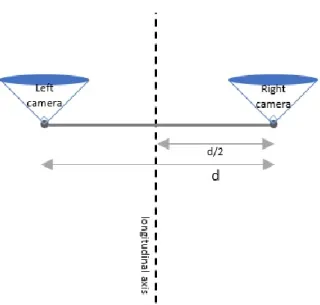
The method can be divided in two different phases: the Detection and the Prevention. The process of obstacle detection is performed by two infrared cameras strategically placed in the aircraft (as described in the figure 1.2). Each camera will provide two angles for each point they detect.

Finalized the first phase, the second phase, named as prevention, begins, which means that the algorithm is initiated.

Figure 1.2- A scheme illustrating the position of the cameras in the aircraft.

1.5 Dissertation Plan

This first chapter consists in: an introduction of the main subject of this dissertation, a description of the objectives to accomplish and a detailed explanation of two theoretical methods.

In the second chapter, a detailed description will be presented of all the necessary steps to complete an anti-collision method based on optical detection. Along with the explanations there will also be illustrative schemes and fundamental equations.

The third chapter will contain all the necessary simulations to properly test the algorithm. For each unique situation, it will be possible to find the initial data, visualise the results (graphics and tables) and analyse a complete discussion of results.

Chapter 2

Development of a Collision Avoidance Method

In this second chapter, a detailed description is presented of all necessary steps to complete an anti-collision method based on optical detection. Along with the explanations will also be illustrative schemes and fundamental equations.

2.1 General Algorithm

Step 1: Conflict Assessment (section 2.2)

For each unique situation, determine based on the angles provided by the cameras if any threat of collision exists. This section is divided in two subsections, which will provide the necessary data to conclude this step.

- Components of the distance vector (subsection 2.2.1)

Calculate all the components of the distance vectors between the aircraft and each point captured by the cameras.

- Vertical and Lateral Distance (subsection 2.2.2)

With the information from the previous subsection, calculate the vertical and lateral distance between the aircraft and each point. An analysis of these distances will allow for the determination of the minimum value of the vertical and lateral distance between the aircraft and the obstacle.

The following steps will only be necessary in case of the existence of a possible threat of collision.

Step 2: Convex Hull Algorithm (section 2.3)

In this step, the Convex Hull method will be used to obtain the convex polygon of each situation. It will allow for visualization of an approximation to the real format of the obstacle.

- Implementation Algorithm (subsection 2.3.1)

Given that the computational tool selected is the Matlab, a specific matlab function will be applied.

Step 3: Conflict Zone (section 2.4)

Determine the area that the aircraft must avoid in order to prevent a possible collision. This section includes two subsections, each one is a specific phase of this step.

- Establish the Sphere (subsection 2.4.1)

The central point and the minimum radius of the sphere encompassing the obstacle will be calculated. Although it is always a three-dimensional situation, the projections in the ‘xz’ and ‘xy’ plan will be used.

- The Final Conflict Zone (subsection 2.4.2)

Having completed the sphere and its projections, it is necessary to find the remaining area to avoid. In three-dimensions, it will be resumed to a conflict cone. However, a different process will be applied, which will allow valuable information for future steps.

Step 4: Assessment of Reality (section 2.5)

The aircraft’s data will be compared with information regarding the conflict zone, previously determined, to analyse the reality of each situation and conclude if the threat of collision is real or not.

The following two steps will only be applied in the situations where the threat is confirmed to be real.

Step 5: Correction Method (section 2.6)

There are three possibilities to modify the aircraft’s path, changing the value of: the heading, the altitude or the velocity. The best option is to alter only one parameter, preferably the heading. However, sometimes it may be necessary to also change the altitude. Both will be analysed and, if needed, new values will be calculated.

- Heading Correction (subsection 2.6.1)

In this subsection, the new value for the aircraft’s heading will be calculated. - Altitude Correction (subsection 2.6.2)

In this subsection, the new value for the aircraft’s altitude will be calculated. Step 6: Variation of a Specific Parameter (section 2.7)

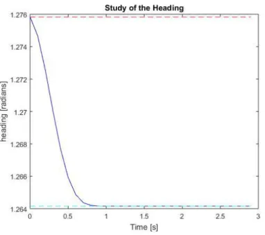
After changing one or both parameters a simple study based on differential equations will be performed to analyse their behaviour over time.

- Heading Variation over time (subsection 2.7.1)

In this subsection, the aircraft’s heading will be studied. - Altitude Variation over time (subsection 2.7.2) In this subsection, the aircraft’s heading will be studied.

Finishing all the steps, the algorithm starts over with new data provided by the cameras. Since the cameras detect points, it is a continuous cycle.

2.2 Step 1: Conflict Assessment

Knowing the exact distance between cameras, ‘d’, along with the data provided by them, it is possible to verify, for each situation, if any threat of collision exists.

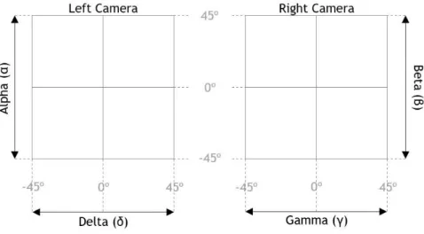
First, it is necessary to calculate the distance vector between our aircraft and each point through the angles provided by the cameras (in the left camera – angles alpha and delta, in the right camera – angles beta and gamma, Figure 2.1). For each point the distance vector is:

where ‘Di ⇀

’ is the distance vector; ‘i’ is the indexing number to identify the point under study and ‘xd’, ‘yd’ and ‘zd’ are, respectively, the ‘x’, ‘y’ and ‘z’ components of the vector. These

three components can also be interpreted as the points coordinates (‘x’, ‘y’ and ‘z’), assuming that the axis origin is on the aircraft.

Figure 2.1- Illustration of an example of the left and right camera images with the respective angles. After calculating all the distances, it is necessary to compare the results with the values of the minimum vertical distance (MVD) and the minimum lateral distance (MLD). If both vertical distance (VD) and lateral distance (LD) are greater than the minimum distance (VD>MVD and LD>MLD) or even if both distances are equal to the minimum distance (VD=MVD and LD=MLD) the danger of collision does not exist so, the aircraft can continue its path. If both distances are less than the minimum distance (VD<MVD and LD<MLD) the danger of collision is a possibility.

Figure 2.2- A three-dimension (x,y,z) scheme to demonstrate visually an example of the distances VD and LD. The blue circle represents the aircraft and the star is a representation of an obstacle.

2.2.1 Components of the distance vector

To correctly determinate all the points’ coordinates there are two parameters essential to the process, the distance from the left camera to the obstacle in terms of the ‘x’ axis, ‘DL’, and the same but from the right camera, ‘DR’.

Figure 2.3- A two-dimension (x,y) scheme illustrating an example of the parameters ‘DL’ and ‘DR’.

In the Figure 2.3, the blue circle represents the aircraft and the star is a representation of an object.

Component ‘y’: the equations to determine the value of this specific component can suffer small modifications depending on the zone where the obstacle is. There are a total of five possible zones.

- if the value of gamma is smaller than zero and delta is greater than zero (first zone, Figure 2.4), we have: ξ_j= - |deltaj| (2.2) φ_j= - |gamma_j| (2.3) DR = cot ξj × d cot φ_j + cot ξ_j (2.4) DL= d - DR (2.5) y = - cot φ_j× DR (2.6)

where, ‘ξ_j’ corresponds to the negative of the absolute value of ‘delta_j’; ‘j’ is the indexing number to identify the point under study; ‘delta’ is the angle provided by the left camera; ‘φ_j’

by the right camera; ‘DR’ is the distance in terms of axis ‘x’ between the object and the right camera (Figure 2.3); ‘d’ is the distance between the cameras; ‘DL’ is the distance in terms of axis ‘x’ between the object and the left camera (Figure 2.3) and ‘y’ is the component to be determined.

Figure 2.4- Scheme illustrating the first zone: the point detected is in the grey zone; which implies that the value of gamma is smaller than zero and delta is greater than zero.

- if the value of gamma is equal to zero and delta is greater than zero (second zone, Figure 2.5), we have:

ξ_j= - |deltaj| (2.7)

DR = 0 (2.8)

DL = d (2.9)

y =- cot ξ_j× DL (2.10)

where, ‘ξ_j’ corresponds to the negative of the absolute value of ‘deltaj’; ‘j’ is the indexing number to identify the point under study; ‘delta’ is the angle provided by the left camera; ‘DR’ is the distance in terms of axis ‘x’ between the object and the right camera (Figure 2.3); ‘d’ is the distance between the cameras; ‘DL’ is the distance in terms of axis ‘x’ between the object and the left camera (Figure 2.3) and ‘y’ is the component to be determined.

Figure 2.5- Scheme illustrating the second zone: the point detected is in the grey line; which implies that the value of gamma is equal to zero and delta is greater than zero.

- if the value of gamma is smaller than zero and delta is equal to zero (third zone, Figure 2.6), we have:

φ_j= - |gamma_j| (2.11)

DR = d (2.12)

DL = 0 (2.13)

y =- cot φ_j× DR (2.14)

where, ‘φ_j’ corresponds to the negative of the absolute value of ‘gamma_j’; ‘j’ is the indexing number to identify the point under study; ‘gamma’ is the angle provided by the right camera; ‘DR’ is the distance in terms of axis ‘x’ between the object and the right camera (Figure 2.3); ‘d’ is the distance between the cameras; ‘DL’ is the distance in terms of axis ‘x’ between the object and the left camera (Figure 2.3) and ‘y’ is the component to be determined.

Figure 2.6- Scheme illustrating the third zone: the point detected is in the grey line; which implies that the value of gamma is smaller than zero and delta is equal to zero.

- if the values of gamma and delta are greater than zero (fourth zone, Figure 2.7), we have: ξ_j= - |deltaj| (2.15) φ_j= - |gamma_j| (2.16) DR = cot ξj× d cot φ_j-cot ξ_j (2.17) DL= d + DR (2.18) y =- cot φ_j× DR (2.19)

where, ‘ξ_j’ corresponds to the negative of the absolute value of ‘deltaj’; ‘j’ is the indexing number to identify the point under study; ‘delta’ is the angle provided by the left camera; ‘φ_j’ corresponds to the negative of the absolute value of ‘gamma_j’; ‘gamma’ is the angle provided by the right camera; ‘DR’ is the distance in terms of axis ‘x’ between the object and the right camera (Figure 2.3); ‘d’ is the distance between the cameras; ‘DL’ is the distance in terms of axis ‘x’ between the object and the left camera (Figure 2.3) and ‘y’ is the component to be determined.

Figure 2.7- Scheme illustrating the fourth zone: the point detected is in the grey zone; which implies that the values of gamma and delta are greater than zero.

- if both values of gamma and delta are smaller than zero (fifth zone, Figure 2.8), we have: ξ_j= - |delta_j| (2.20) φ_j= - |gamma_j| (2.21) DR = cot ξj× d cot ξ_j- cot φ_j (2.22) DL= DR – d (2.23) y =- cot φ_j× DR (2.24)

where, ‘ξ_j’ corresponds to the negative of the absolute value of ‘deltaj’; ‘j’ is the indexing number to identify the point under study; ‘delta’ is the angle provided by the left camera; ‘φ_j’ corresponds to the negative of the absolute value of ‘gamma_j’; ‘gamma’ is the angle provided by the right camera; ‘DR’ is the distance in terms of axis ‘x’ between the object and the right camera (Figure 2.3); ‘d’ is the distance between the cameras; ‘DL’ is the distance in terms of axis ‘x’ between the object and the left camera (Figure 2.3) and ‘y’ is the component to be determined.

Figure 2.8- Scheme illustrating the fifth zone: the point detected is in the grey zone; which implies that the values of gamma and delta are smaller than zero.

Component ‘z’: the process to calculate this component may vary according to the values of the parameters ‘DL’ and ‘DR’ and it can be resumed in two possible cases, which are:

- if, independently of the value of ‘DL’, the value of ‘DR’ is greater than zero:

where ‘hypotenuse’ is the vector distance between our aircraft and the object when projecting in the ‘xy’ plane; ‘DR’ is the distance in terms of axis ‘x’ between the point and the right camera (Figure 2.3); ‘y’ is the component calculated before; ‘z’ is the component to be determined and ‘beta’ is an angle provided by the right camera.

- if the value of ‘DR’ is equal to zero and ‘DL’ is equal to ‘d’:

hypotenuse = √(DL2 + y2) (2.27)

z = tan(alpha_j) × hypotenuse (2.28)

where ‘hypotenuse’ is the vector distance between our aircraft and the object when projecting in the ‘xy’ plane; ‘DL’ is the distance in terms of axis ‘x’ between the point and the left camera (Figure 2.3); ‘y’ is the component calculated before; ‘z’ is the component to be determined and ‘alpha’ is an angle provided by the left camera.

hypotenuse = √(DR2 + y2₎ (2.25)

Component ‘x’: for this last component three possible scenarios exist to determine: - if DR>DL:

where ‘x’ is the component to be determined; ‘DR’ is the distance in terms of axis ‘x’ between the object and the right camera (Figure 2.3) and ‘d’ is the distance between the cameras.

- if DR<DL:

where ‘x’ is the component to be determined; ‘DL’ is the distance in terms of axis ‘x’ between the object and the left camera (Figure 2.3) and ‘d’ is the distance between cameras.

- else:

where ‘x’ is the component to be determined.

2.2.2 Vertical and Lateral Distance

The VD between our aircraft and each point corresponds to the component ‘z’. However, in terms of the LD it is necessary to calculate based on the ‘x’ and ‘y’ coordinates. Vertical and lateral distance for each point ‘j’:

where ‘VDj’ is the vertical distance between our aircraft and the point ‘j’; ‘j’ is the indexing number to identify the point; ‘zj’ is the component ‘z’ of the point ‘j’; ‘LDj’ is the lateral distance between our aircraft and the point ‘j’; ‘xj’ and ‘y_j ’ are respectively the ‘x’ component and ‘y’ component of the point ‘j’.

x = -(DR- (d 2) ) (2.29) x = DL - (d 2) (2.30) x = 0 (2.31) VDj = zj (2.32) LD_j = √((x_j)2 + ( y_j )2) (2.33)

2.3 Step 2: Convex Hull Algorithm

A definition of convex hull method and three of the most important algorithms were previously exposed. In this section, it will be applied in the process to determine the specific area that the aircraft must avoid. For each situation, we will determine the respective convex polygon. However, the convex polygon does not necessarily represent the real format of the obstacle being studied, it is just an approximation to the actual format.

2.3.1 Implementation Algorithm

Since the computational tool chosen for this work was Matlab the determination of the convex hull for each case will be through one specific Matlab function named ‘convhull’, which allows not only to find the specific points that are vertices but also to graphically demonstrate the convex hull.

Algorithm used for the convex hull method: assuming equal ‘y’ to all points (2D).

where ‘k’ represents the convex hull function to determine; ‘convhull(x,z)’ is the matlab function; ‘x’ and ‘z’ are, respectively, the vector with all the ‘x’ and ‘z’ coordinates of the points.

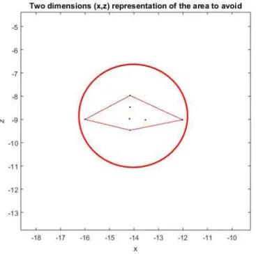
2.4 Step 3: Conflict Zone

The determination of the convex hull is just the first step to accomplish a second objective, finding the specific area to avoid, there are two more necessary steps: first, establish the sphere involving the obstacle and, second, the cone, which represents the conflict zone.

2.4.1 Establish the Sphere

In the process todetermine the convex hull the points are separated by two categories: inside the convex hull and vertices. Knowing the points belonging to the category ‘vertices’ it is possible to calculate a central point of the convex hull by the average of those points coordinates. If this same procedure is applied to all the points, instead of only the ‘vertices’, the result is the midpoint of the initial set, which will be the sphere centre.

The best method to correctly define the minimum radius possible is to calculate the distance between the centre and each other point, then the biggest distance calculated is the minimum radius. However, in terms of security and safety issues a safety margin must be added to the minimum radius calculated before.

In terms of algorithm: Midpoint:

where ‘cx’ is the ‘x’ coordinate of the central point; ‘x(j)’ is the ‘x’ coordinate of the point ‘j’;

‘j’ is the indexing number to identify the point; ‘nj’ is the total number of points; ‘cz’ is the ‘z’

coordinate of the central point and ‘z(j)’ is the ‘z’ coordinate of the point ‘j’. Distance between the midpoint and each point:

where ‘dis(j)’ is the distance between the central point and the point ‘j’; ‘j’ is the indexing number to identify the point; ‘x(j)’ is the ‘x’ coordinate of the point ‘j’; ‘cx’ is the ‘x’

coordinate of the central point; ‘z(j)’ is the ‘z’ coordinate of the point ‘j’ and ‘cz’ is the ‘z’

coordinate of the central point. Minimum radius:

where ‘r’ is the radius of the circumference; ‘ω’ is the safety margin and ‘dismax’ is the

maximum distance previously calculated.

This sphere can be projected in any plan and it will always have the same radius and centre coordinates.

2.4.2 The Final Conflict Zone

In a three-dimensional case, the result would be a cone and just two things are necessary, a base and a height, to define it. The cone base is a circumference, whose’ characteristics were previously determined. And the cone height corresponds to the norm of the vector distance between the aircraft and the sphere centre (midpoint). This vector can be calculated since both aircraft’s coordinates and the centre coordinates are known.

cx = ∑x(j) nj (2.35) cz = ∑z(j) nj (2.36) dis(j) =√(x(j) - c_x)2 _{+ (z(j) - c} z)2 (2.37) r = (1-ω)× dis_max (2.38)

In terms of two-dimensions, the cone will be projected on the ‘xy’ plane and will correspond to a circumference and two specific lines, which must be tangent to the circumference and pass on the origin. To determine the equations of the lines it is essential to first find the only two points belonging both to one line and to the circumference. The equations to find the two necessary points are:

where ‘r’ is the circumference radius; ‘px’ is the ‘x’ coordinate of the tangent point; ‘cx’ is the

‘x’ coordinate of the central point; ‘py’ is the ‘y’ coordinate of the tangent point; ‘cy’ is the

‘y’ coordinate of the central point and ‘hp’ is the distance vector between the aircraft and the

new point. The result of this equation is two sets of ‘x’ and ‘y’ coordinates corresponding to two different points.

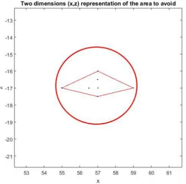
Figure 2.9- An example of a two-dimension (x,y) representation of the specific area to avoid. The blue circle represents the aircraft and the star is a representation of an obstacle.

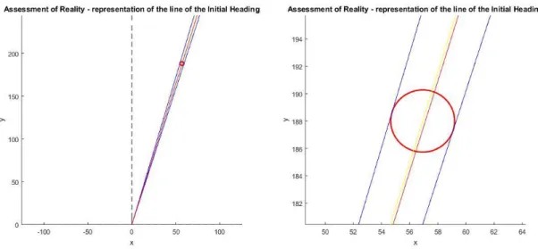
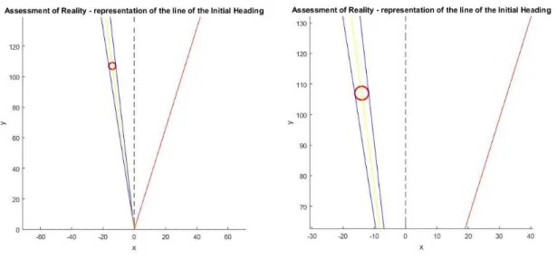
2.5 Step 4: Assessment of Reality

After finding the specific area that the aircraft must avoid the following step is to compare it with the actual aircraft’s heading. Two results are possible: the aircraft’s heading is in the safe zone outside the cone or it is coincident with the conflict zone. The first result allows for concluding that the danger of collision is not real, which means that there is no need of changing anything in the aircraft’s path. On the other hand, the second result confirms the existence of danger of collision and the necessity of quickly change the aircraft’s path.

r =√(p_x- cx) 2 + (p_y- cy) 2 hp=√px2 + py2 (2.39) (2.40)

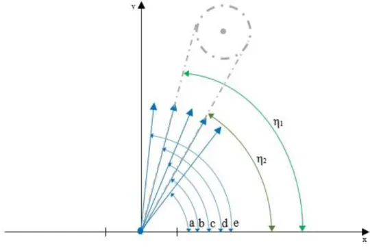
The angles named eta1 (η1) and eta2 (η2) are, respectively, the angles that the left border and

the right border of the conflict zone makes with the ‘x’ axis (Figure 2.10). They will be needed in the process of assessment of reality, which will be performed by comparing angles.

In terms of algorithm:

- if heading is greater than eta2 (η2) and smaller than eta1 (η1): the danger of collision is

real because the heading is exactly inside the cone (possibility ‘c’ in figure 2.10). - if heading is equal to eta1: although the aircraft’s heading is on the left border it is still

considered inside the cone, so the danger of collision is real (possibility ‘d’ in figure 2.10).

- if heading is equal to eta2: this situation is similar to the previous case, the aircraft’s

heading is on the right border so, the danger of collision is real (possibility ‘b’ in figure 2.10).

- if the heading does not coincide with any of the previous options: the logical conclusion is that the aircraft’s heading is in the safe zone (possibility ‘a’ and ‘e’ in figure 2.10).

Figure 2.10- An illustration of the possibilities in the assessment of reality process.

The zone delimited by the grey lines is the conflict zone. The green curve lines describe the angles eta1 (η1) and eta2 (η2). The blue arrows, which each angle is represented by a letter

(‘a’, ‘b’, ‘c’, ‘d’ and ‘e’), represent five general possibilities to the aircraft’s heading. The possibilities ‘a’ and ‘e’ are free from danger of collision. The other three, ‘b’, ‘c’ and ‘d’, represent situations where the danger of collision is real. The blue point in the origin represents our aircraft.

2.6 Step 5: Correction Method

The change in the aircraft’s path must be quick and effective in order to prevent an imminent collision. So, it is necessary to find the best solution for each case. In fact, there are three possibilities to implement as a correction and each one involves a different flight characteristic, they are: the first is to change the value of the aircraft’s heading, the second instead of heading the decision is to change the altitude and the last possibility is to modify the velocity. However, the third possibility is normally avoided, used only as a last resort. In fact, the ideal case is to change only the value of one flight characteristic, usually the heading, because the more features are changed the more complex it is to deal with the aircraft and its control. In some cases, when the heading is changed, the altitude must also be corrected, it will depend on if the value of the aircraft’s altitude along with a safety margin corresponds inside the circumference.

Next, in this paper a detailed description will be presented for the heading correction and the altitude correction.

2.6.1 Heading Correction

The heading correction is a simple and assertive method well suited to any collision avoidance situation. First, it is necessary to comprehend if the value of the heading, which means the angle, should be increased or decreased. That decision must be made by comparisons: if the heading is closest or even equal to the left limit of the area to avoid the angle must increase, but if it is closest or even equal to the right limit the value of the angle must decrease and there is also the rare possibility of being exactly in the middle in this case the option will be to increase (Figure 2.11).

Previously, both eta1 (η1) and eta2 (η2) were introduced, now one more angle is necessary. The

angle etac (ηc) is the angle that the central line, which divides the conflict zone exactly in half

(left and right side), makes with axis ‘x’. New value of heading

In this section, a description of the method to calculate the new value for the heading will be introduced. The first step is to assess if the value of heading is between the limits or equal to one limit. If it is equal to one limit the value can be automatically calculated but if it is inside limits it is necessary to proceed to one more process of comparisons. In this second comparison process we will evaluate if the heading is in the left part of the conflict zone or in the right part, for that the angle of heading will not only be compared to the angles that each limit makes with the axis ‘x’ but also compared with the angle etac (ηc).

In terms of algorithm:

- if heading is equal to eta1 (possibility ‘e’ in Figure 2.11) it is possible to immediately calculate

the new value of heading, in this case it is necessary to increase the value of heading so it assumes a higher value than eta1:

where ‘headingnew’ is the new value of heading to be calculated; ‘λ’ is a constant with the

smallest value possible (0 < λ≪1) and ‘heading’ is the initial value.

- if heading is equal to eta2 (possibility ‘a’ in Figure 2.11), just like in the previous possibility,

the calculation of the new value is immediate, in this case it is necessary to decrease the value of heading so it assume a smaller value than eta2:

where ‘headingnew’ is the new value of heading to be calculated; ‘λ’ is a constant with the

smallest value possible (0 < λ≪1) and ‘heading’ is the initial value.

- if we have heading greater than eta2 and smaller than eta1it means that heading is inside the

limits so, we proceed to the second process of comparison where three possible cases exist: - if heading is greater than eta2 and smaller than etac (possibility ‘b’ in Figure 2.11) it

is in the right side of the conflict zone so, in this case it is necessary to decrease the value of heading in order to assume a smaller value than eta2:

heading_new = heading - (1+λ)×(heading-eta2) (2.43) where ‘headingnew’ is the new value of heading to be calculated; ‘heading’ is the initial value;

‘λ’ is a constant with the smallest value possible (0 < λ≪1) and eta2 is an angle.

- if heading is greater than etac and smaller than eta1 (possibility ‘d’ in Figure 2.11) it

is in the right side of the conflict zone so, in this case it is necessary to increase the value of heading in order to assume a higher value than eta1:

where ‘headingnew’ is the new value of heading to be calculated; ‘heading’ is the initial value;

‘λ’ is a constant with the smallest value possible (0 < λ≪1) and eta1 is an angle.

- if heading is equal to etac (possibility ‘c’ in Figure 2.11), it is exactly in the middle of

the conflict zone, although rare it is a possible situation, so, in this case the decision is to decrease the value of heading in order to assume a smaller value than eta2:

heading_new = (1+λ)×heading (2.41)

heading_new = (1-λ)×heading (2.42)

heading_new = heading + (1+λ)×(eta1-heading) (2.44)

where ‘headingnew’ is the new value of heading to be calculated; ‘heading’ is the initial value;

‘λ’ is a constant with the smallest value possible (0 < λ≪1) and eta2 is an angle.

Figure 2.11- This figure is an illustration of the existing possibilities in the process of calculating the new value for the aircraft’s heading.

The zone demarked by the grey lines is the conflict zone. The green and curve lines describe the angles eta1 (η1), etac (ηc) and eta2 (η2). The blue arrows, which each angle is represented

by a letter (‘a’, ‘b’, ‘c’, ‘d’ and ‘e’), represent the five possibilities to the aircraft’s heading when the danger of collision is real. The blue point in the origin represents our aircraft.

2.6.2 Altitude Correction

This correction method will be applied only if the aircraft’s altitude coincides inside the area to avoid in terms of ‘xz’ plane, so before calculating the new altitude it will be necessary to analyse the situation. Just like in the heading correction, it is fundamental to understand if the value of altitude must increase or decrease to calculate the most appropriate new value for each case.

New value of altitude

To calculate the new value for the altitude it is essential to know if the obstacle captured by the cameras is, relatively to our aircraft, higher, lower or at the same altitude. Since all point’s coordinates and distance vectors were calculated on the basis of our aircraft’s position, this task is complete by analysing the value of the ‘z’ coordinate of the central point of the circumference.