IMPACTS OF SOUTHERN HEMISPHERE WESTERLIES ON THE BRAZIL CURRENT AT 30
◦S
Jessica S. Carvalho
1, Fabricio S. C. Oliveira
2and Edmo J. D. Campos
1ABSTRACT.Previous studies have pointed out an intensification of the global western boundary currents induced by changes in the wind-stress curl patterns over the oceans. The Brazil Current (BC) is the western boundary current into the South Atlantic Subtropical Gyre, which flows southwards along the Brazilian coast. A numerical model is used to investigate the response of BC to this change in wind forcing between 1960-2010, across 30ºS. The results found here support the increasing trend noticed in the wind-stress curl and a poleward migration of the South Hemisphere westerlies in the past decades. The residual transport of BC at 30◦S is composed by
its southward main flow and the northward branch of a recirculation cell (Rec) east of the BC. Both the BC and Rec transports showed a decrease trend of 0.10 Sv dec−1
and 0.28 Sv dec−1, respectively. It suggests a southward migration of Rec in response to changes in the westerlies. The results also indicate a relative intensification in the western boundary transport and a strengthening in the South Atlantic Subtropical Gyre.
Keywords: western boundary current, meridional transport, HYCOM.
RESUMO.Estudos anteriores apontam para uma intensificação das correntes de contorno oeste globais induzidas por mudanças no rotacional do estresse do vento sobre os oceanos. A Corrente do Brasil (CB) é a corrente de contorno oeste do giro Subtropical do Atlântico Sul, que flui para sul ao longo da costa brasileira. Um modelo numérico é usado para investigar a resposta da CB às mudanças na forçante do vento entre 1960-2010, ao longo de 30◦S. Os resultados encontrados aqui
suportam a tendência de aumento observada no rotacional do estresse do vento e a migração para o polo dos ventos de oeste do hemisfério sul nas últimas décadas. O transporte residual da CB em 30ºS é composto pelo seu fluxo principal para sul e o braço para norte de uma célula de recirculação (Rec) a leste da CB. Ambos os transportes da CB e Rec mostraram uma tendência de redução de 0,10 Sv dec−1e 0,28 Sv dec−1, respectivamente. Isto sugere uma migração para sul da Rec
em resposta às mudanças dos ventos de oeste. Os resultados também indicam uma relativa intensificação do transporte na borda oeste e um fortalecimento do giro Subtropical do Atlântico Sul.
Palavras-chave: corrente de contorno oeste, transporte meridional, HYCOM.
1Universidade de São Paulo, Instituto Oceanográfico, Praça do Oceanográfico, 191, São Paulo, 05508-120, SP, Brazil. Phone: +55(11)3091-6578 - E-mails:
[email protected], [email protected]
2Universidade Federal do Rio Grande, Instituto de Oceanografia, Avenida Itália, km 08, Rio Grande, 96203-900, RS, Brazil. Phone: +55(53)3233-6860 - E-mail:
INTRODUCTION
Evidences from several atmospheric models and observations have pointed out to a poleward migration and an intensification of the Southern Hemisphere westerlies in mid and high latitudes over the past decades (Thompson & Solomon, 2002; Marshall, 2003; Toggweiler, 2009). Sen Gupta et al. (2009), based on climate forecast models, showed a continuous positive trend in magnitude of westerlies along the current century. Other studies associated this atmospheric variability to the ozone hole and to the increase in the concentration of greenhouse gases (Marshall et al., 2004; Cai & Cowan, 2007).
A significant part of the sub-inertial ocean variability is driven by wind forcing (Moore, 1999), thus changes in the upper ocean circulation such as the strengthening in all subtropical ocean gyres previously reported by Roemmich et al. (2007) are expected. The intensification of wind-stress over the past century may have increased the equatorward flow far from the continental borders and inducing an increase in the poleward flow associated to the western boundary currents (Wu et al., 2012). Curry & McCartney (2001) observed an increase of about 30% in the Gulf Stream and North Atlantic Current associated to changes in the atmospheric forcing. Similar increasing trends were observed in the Brazil Current (BC) (Wu et al., 2012). Wu et al. (2012) also observed a poleward shift of about –2º±0.6º in the zero wind-stress curl line over the South Atlantic, which demarcates the limits of the subtropical ocean gyre.
The BC is the western boundary current into the South Atlantic Subtropical Gyre, which flows southward along the Brazilian coast and feeds the upper branch of the Atlantic Meridional Overturning Circulation (AMOC). While it flows south, the BC carries warmer subtropical waters to high latitudes where it collides with the northward colder waters from the Malvinas Current (MC) between 33ºS–40ºS (Matano et al., 1993), in the region called the Brazil-Malvinas Confluence (BMC). The BC transport is considered smaller and shallower than other western boundary currents, although it increases as it runs southward (Gordon & Greengrove, 1986; Stramma, 1989; Stramma et al., 1990; Pickard & Emery, 2016). Stramma (1989) used historical hydrographic data to compute geostrophic transports between 5–6.5 Sv (1 Sv = 1x10⁶ m3s−1 in the upper 500 m near 20ºS.
South of 24ºS, the BC flow increases by about 5% per each 100 km until reaches its maximum between 19–22 Sv in the BMC (Stramma et al., 1990). Near 30ºS the intensification of the BC transport shows up associated to a recirculation cell (Rec) that has been observed in hydrographic, ADCP and drifter data
(Olson et al., 1988; Stramma et al., 1990; Biló et al., 2014). Based on hydrographic data, Stramma (1989) computed a geostrophic transport of 7.5 Sv associated to Rec in the upper 800 m.
Although the air-sea exchanges have been exhaustively studied in the Pacific and North Atlantic oceans, the South Atlantic is pointed out as one of the keys for understanding the role of the oceans in climate change (Garzoli et al., 2013). The South Atlantic is particularly important due to its equatorward heat transport from subtropical regions, that provides important interhemispheric exchanges of oceanic proprieties to the North Atlantic. In this context, it becomes essential to enhance the knowledge about the effect of atmospheric forcing into the ocean circulation focused on the western boundary currents. Based on that, the objective of this paper is to investigate what is the influence of wind-stress patterns in the meridional volume transport over the South Atlantic western boundary at 30ºS.
MATERIAL AND METHODS Model Description
A simulation using the HYbrid Coordinate Ocean Model (HYCOM) (Bleck, 2002) was implemented to the area 98ºW–114ºE and 65ºS–60ºN, which includes the Atlantic and Indian Ocean basins (Fig. 1). Despite the focus of this study is on the South Atlantic, the Indian Ocean was included because the Agulhas system directly impacts the South Atlantic meridional transports. HYCOM is an oceanic general circulation model that solves the hydrostatic primitive equations in a spatial mesh using a generalized (hybrid) vertical coordinate.
The numerical experiment, hereafter HYCOM, has a
1/4–degree horizontal resolution and 22 hybrid vertical layers.
The mixing throughout the water column was computed by the K-profile parameterization (KPP) (Large et al., 1994), and the bathymetry was defined by the non-smoothed NOAA/NGDC ETOPO5 5. HYCOM was initialized from rest using thermohaline fields from Levitus Climatology. A barotropic transport of 148 Sv was imposed in and out across the western and eastern boundaries to represent the Antarctic Circumpolar Current (ACC). This imposed transport is in agreement with those reported by Cunningham et al. (2003) across the Drake Passage. The Indonesian straits were closed, with no Indonesian Throughflow. The temperature and salinity at the open lateral boundaries were relaxed to the climatology, using a two-degree wide buffer zone and 120 days relaxation time. The northern and southern boundaries were closed, with no barotropic inflow or outflow, and temperature and salinity also relaxed to climatology. HYCOM
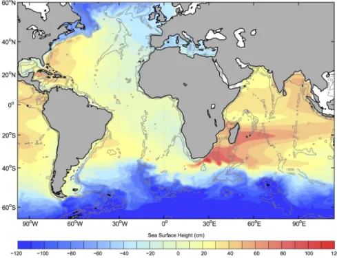
Figure 1 – Map of sea surface height from HYCOM representing the model domain, and isobaths of 1000 m and 3000
m in gray
was warmed up for 10 years from COADS monthly climatology, and these results were then used as initial conditions for the “dated” experiment, forced with monthly means of the National Centers for Environmental Prediction and National Center for Atmospheric Research (NCEP/NCAR) Reanalysis 1 (Kalnay, 1996). The reanalysis fields include wind-stress, longwave radiation, shortwave radiation, precipitation and humidity.
The evaporation and sensible heat are estimated from the precipitation and air temperature respectively. The sea surface salinity is weakly relaxed to climatology and the sea surface temperature (SST) is free. The model is run from 1948 to 2010, and due to the “warm” start-up, the results are based on the period 1960–2010.
Satellite Data
Despite this study is not focused on model evaluation, satellite-based data were used to access the model’s accuracy in reproducing the ocean surface. The SST data were collected by the Advanced Very High Resolution Radiometer (AVHRR) on the NOAA’s satellites, processed by Pathfinder Project and downloaded from the Physical Oceanography Distributed Active Archive Center at the NASA’s Jet Propulsion Laboratory (PO.DAAC/JPL). This data set corresponds to daily global
images at the 1 km resolution for the period 1985–2010. The altimetry records, hereafter sea surface height (SSH), correspond to the gridded multimission product of the global Maps of Absolute Dynamic Topography (MADT) and absolute geostrophic velocities processed by Ssalto/Duacs, and downloaded from Archiving, Validation, and Interpretation of Satellite Oceanographic data (AVISO). The SSH data set is distributed in a daily 1/4–degree resolution for the period
1992–2010. In addition, the surface eddy kinetic energy (EKE) was derived from altimeter data to compose the further analysis.
The spatial resolutions of the SST and SSH images were lowered by subsampling to match that of the model. The subsampled images were then averaged for representing the spatial variability of these data, and simple model-data differences were computed to access how well the model reproduces the surface fields.
In-situ Data
For observing the ocean subsurface variability, temperature and salinity data provided by autonomous profiling floats from Argo Program were used. The Argo data used here corresponds to a monthly global gridded data distributed by University of California San Diego’s Scripps Institution
of Oceanography (UCSD/SIO), in four-dimensional fields of temperature and salinity, 1-degree resolution, and 58 levels between 2.5–2000 dbars from the period 2004–2010 (Roemmich & Gilson, 2009). Argo data were also interpolated to match the model resolution.
Reanalysis Data
The wind-stress curl was computed over the South Atlantic between 20ºE–70ºW and 0º–60ºS using the surface wind fields from NCEP/NCAR Reanalysis 1. These fields are distributed in a global T62 Gaussian grid in a monthly time resolution for the period 1960–2010. Time series and trends of the wind-stress curl over the South Atlantic and the zero wind-stress curl lines were investigated for the same period. Previous studies have presented discontinuities and dubious trends in the earlier NCEP/NCAR reanalysis over high latitudes due to the absence of complementary data before 80’s; satellite records in this case (Sturaro, 2003). The use of NCEP/NCAR reanalysis as the model forcing and to study the impact of the wind in the ocean circulation implies in a previous autocorrelation between them, even though observations support the intensification and the poleward shift in the South Hemisphere westerlies (Bromwich & Fogt, 2004; Renwick, 2004).
Sverdrup Theory
The first attempt to estimate the wind influence in the BC transport was performed by the Sverdrup theory. The Sverdrup balance corresponds to the linear vorticity equation derived from a steady state and vertically integrated from surface to a null movement level
β.V =(∇ ×~τ).k ρ0
, (1)
where β =d f/dy is the beta parameter, V is the meridional
volume transport given by Sverdrup balance,τis the wind-stress
vector, k is the unit vector in the vertical direction, andρ0is the
seawater density. The Eq. (1) shows that the meridional transport depends directly on the wind-stress curl.
In the South Atlantic Subtropical interior region, the Sverdrup transport is northward since wind-stress curls take positive values. Therefore, southward transport in the western boundary region is given as a compensating flow of the Sverdrup transport in the interior region (Pedlosky, 2013). At this point, the total Sverdrup’s return transport at a given latitude may be compared to a local western boundary current (Cai et al., 2005; Saenko et al., 2010), in the South Atlantic it can be comparable to
the BC transport. Thereby to estimate the BC transport from wind data at 30ºS, hereafter called BCSV,Eq.(1) is integrated from the
African continent towards the western limit of the South Atlantic.
Meridional Transport from HYCOM
The BC modeled transport was analyze at 30ºS, where its flow is still organized and preferentially barotropic, hereafter called BCHYCOM. The zonal limits of integration to delimit the BCHYCOMwas
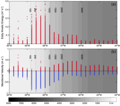
based on the zonal distribution of the meridional velocity and its EKE across 30ºS, assuming that the western boundary currents are the most energetic and stronger currents in the ocean (Beal et al., 2011). The region between 47.25ºW–48.75ºW showed the highest values of EKE and negative velocities clearly associated to the southward BC flow, while a northward flow with moderate EKE values is observed east of BC between 46.00ºW–47.25ºW (Fig. 2).
The northward transport is related to the Rec flow previously reported (Stramma, 1989). Both southward and northward flows can also be observed in the mean EKE and meridional velocity in the mixed layer (Fig. 3a,b). The BCHYCOMand Rec transports were
computed by the vertical integration of the meridional velocities from HYCOM to include the Tropical Water (TW), South Atlantic Central Water (SACW) and Antarctic Intermediate Water (AAIW), that is from surface to the layer boundary of the AAIW. The lower boundary of AAIW is defined as the depth equivalent to isopycnal 27.35 kg m−3(Schmid et al., 2000) (Fig. 3).
These authors affirm that this isopycnal represents well the lower interface of the AAIW, and it should not change significantly within the South Atlantic. The BCHYCOMand Rec can be expressed
according to, T= Z xW xE Z 0 −h v(x, z)dxdz, (2) where v is the model meridional velocity from HYCOM, h is the lower boundary of AAIW, xEand xW are the eastern and western
limits of 47.25ºW–48.75ºW for BCHYCOMand 46.00ºW–47.25ºW
for Rec. All time series were filtered using a1/4–year low-pass
filter to reduce the noise, and their respective trends are statistically significant at the 95% confidence level.
RESULTS Model Evaluation
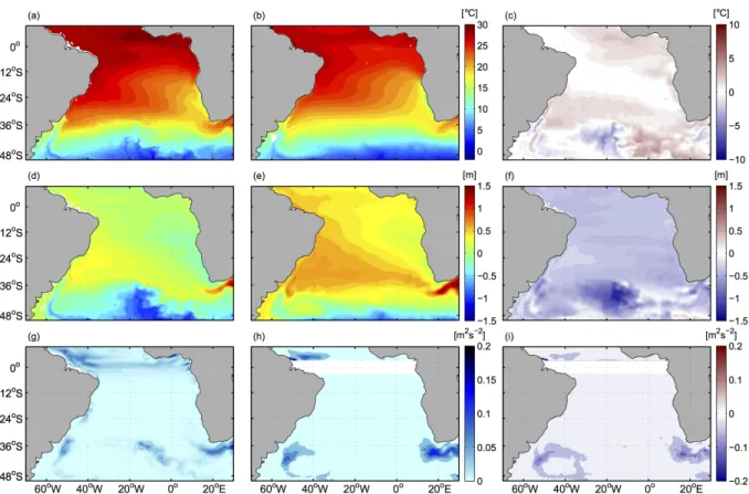
Model-data comparisons of SST, SSH, and EKE are used to evaluate performance in simulating the real ocean (Fig. 4). Positive differences indicate overestimation by the model, while
Figure 2 – Zonal distribution of (a) EKE and (b) meridional velocity from surface to isopycnal 27.35 kg m−3at 30ºS.
The red and blue dots correspond to positive and negative values, respectively, and the shades of gray on background are the local bathymetry.
Figure 3 – (a, b) Time-mean EKE (m2s−2) and meridional velocity (m s−1) in the mixed layer at 30ºS on background, respectively. Vectors are the mean velocity field
in m s−1and the black lines are the isobaths of 100, 2000 and 3000 m. (c) Time-mean meridional velocity at 30ºS representing the areas used to compute the BC HYCOM
Figure 4 – Time-mean maps of SST (top), SSH (middle) and EKE (bottom) from HYCOM (first column), satellite-based data (second column) and HYCOM–satellite
(third column). The SST maps correspond to the time period 1985-2010 and SSH and EKE to 1992-2010.
negatives indicate underestimation. HYCOM reproduces well the satellite-based SST in most of the domain, with slightly warmer waters north of 36ºS and a few sites of colder waters in the south (Fig. 4a-c). In general, the SST differences ranged from -2ºC to 2ºC, falling close to zero within the Subtropical Gyre. A model-data correlation in the South Atlantic basin showed a coefficient of 0.97 (not shown). The BMC and the Zapiola Anticyclone (ZA) regions were well captured by the model, although they are up to 3ºC warmer than observations. The thermal gradients of the Agulhas Retroflection (AR) and the Benguela upwelling zone were also overestimated in 2ºC by the model. Below 36ºS and over the Mid-Atlantic Ridge (MAR) HYCOM shows maxima differences of up to ± 4ºC. The simulated SSH underestimated those values observed by altimetry, except in a small area south of Southern African coast, where the differences were slightly positives (∼ 0.1 m). Nevertheless, HYCOM retained the main observed mesoscale variability, and showed a robust correlation coefficient (r=0.84) (not shown). The variability in the AR and BMC regions were also well
captured, although underestimated by up to 0.5 m. About 60% of the altimetry-based EKE was explained by the model, while it increases to 70% in the BMC region. The BMC and AR gathers a lot of energy from the eddy-like features released by the local western boundary currents, and larger differences are already expected in these regions.
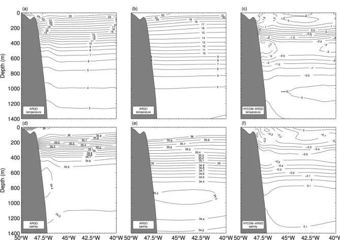
The vertical thermohaline structure across 30ºS was also investigated and are presented in Figure 5. The isotherm patterns from Argo were satisfactorily reproduced between the surface and 1400 m, although the thermocline was slightly shallower and narrower in the model. Temperatures in the upper 300 m were slightly overestimated by the model, with differences generally ranging from 0.5ºC to 1.5ºC and peaks of 2ºC at the surface. Keep in mind that these Argo fields do not present measurements properly on the surface (∼ 0 m) and over the continental shelf; the two regions where the differences were expected to be higher. Isotherms between 400–600 m depth are underestimated by up to 3.5ºC, and those below 600 m did not exceed 2ºC. The slanted isotherms found west of 46ºW are supposedly associated to
interpolation applied to Argo data and the lack of data over the shelf. The modeled salinity showed a shallower and narrower halocline compared to observations, even though it reproduces the salinity minimum between 800–1000 m associated to the AAIW (Fig. 5d). Arruda et al. (2013) found the same AAIW signature between 500–1500 m for latitudes south of 28º S using a numerical model. Since the model simulated a broader AAIW, the halocline was confined to the upper 400–500 m and the differences just below this layer are larger. Near the surface, the model was quite similar to data, showing an increase of up to -0.5 in the differences around the middle of halocline (∼ 500 m). Below 500 m, the differences decrease again and range from -0.1 to 0.1 around 1400 m. Despite the coarser vertical resolution of HYCOM, it successfully represents the thermohaline structure observed by Argo at 30ºS.
Trends in the South Hemisphere westerlies
Time series of wind-stress and wind-stress curl derived from NCEP/NCAR Reanalysis were used to observe the long-term variability of the westerlies over the South Atlantic. Negative trends of wind-stress in mid-latitudes and high positive trends south of 45ºS suggest a weakening in the mid-latitude westerlies and a strengthening in the subpolar westerlies (Fig. 6). The wind-stress patterns cause an intensification of mean wind-stress curl between 10ºS and 50ºS, with a positive trend of 0.1×10⁻⁸
N m−3 dec−1 which explains about 54% of the total variance
(Fig. 6b).
A southward migration of the whole South Atlantic subtropical ridge is also observed in Fig. 6(a), and it is represented by the poleward shift of the mean zero wind-stress curl lines between 1960s (black lines) and 2000s (yellow lines). The white line is the long-term average. The southward migration of the wind-stress curl is about -0.31º per decade and represents 20.8% of the total variance (Fig. 6c). Wu et al. (2012) estimated a total migration of the wind-stress curl line of about –2º±0.6º over the past century. This migratory pattern leads to a reduction of the Southern Hemisphere westerlies and positive trends in the Southern Annular Mode (SAM) index (Thompson & Solomon, 2002; Toggweiler, 2009; Wu et al., 2012). The correlation between the mean wind-stress curl and SAM index during austral summer was about 0.6 (not shown).
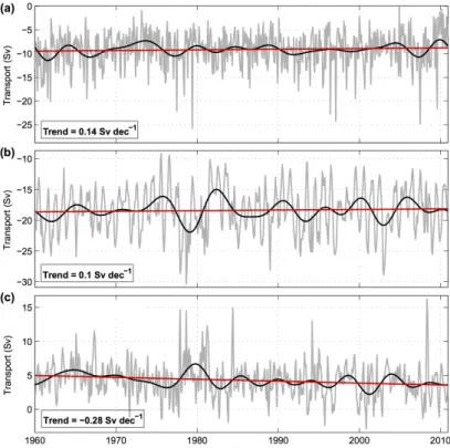
a minimum value of -25.79 Sv. The negative value indicates a southward transport. Despite the intensification of the wind-stress curl over the South Atlantic (Fig. 6), the Sverdrup transport showed a decreasing trend of about 0.14 Sv dec−1(Fig. 7a), which
is in accordance with the local trend of –0.04×10⁻⁸N m−3dec−1
observed in the zonally averaged wind-stress curl at 30ºS (not shown). It suggests that the BCSV responses faster to the local
wind forcing instead of the regional one.
This decreasing trend in the wind-stress curl is corroborated by Pontes et al. (2016), that also found a decrease in the interior transport of the South Atlantic basin supposedly related with the Sverdrup transport.
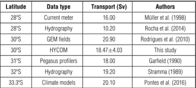
The BCHYCOM transport at 30ºS ranged from -8.43 to
-30.37 Sv. The average of -18.47±4.03 Sv is more realistic than that found by Sverdrup theory, and corroborates previous hydrographic observations obtained close this region (Stramma, 1989; Garfield, 1990; Müller et al., 1998). A brief summary of previous estimates of the BC transport is presented in Table 1. On the other hand, the decreasing trend of about 0.1 Sv dec−1is
compatible with that one found using the Sverdrup theory (0.14 Sv dec−1) (Fig. 7).
A cross-correlation between the transports computed by both methods showed a maximum coefficient of about 0.6 for a lag of 2 years. A similar time lag between the wind fields and thermodynamic ocean variables was also observed by (Qiu & Chen, 2006; Roemmich et al., 2007; Hill et al., 2010) in the region dominated by the East Australian Current. According to these authors, this time-scale variability is a response of ocean planetary waves, which links the large-scale wind variability to the anomalies in the western boundary current transports. The differences and observed the lag between BCHYCOM and BCSV
transports shows the inability of the Sverdrup theory to an instantaneous response of the ocean to the wind-stress.
Table 1 – Summary if previous estimates of the BC transport near to 30ºS.
Latitude Data type Transport (Sv) Authors
28ºS Current meter 16.00 Müller et al. (1998) 28ºS Hydrography 10.20 Rocha et al. (2014) 30ºS GEM fields 20.90 Rodrigues et al. (2010)
30ºS HYCOM 18.47±4.03 This study
31ºS Pegasus profilers 18.00 Garfield (1990) 32ºS Hydrography 19.20 Stramma (1989) 33.3ºS Climate models 20.10 Pontes et al. (2016)
Figure 5 – Mean vertical profiles of temperature (top) and salinity (bottom) from HYCOM (a, d), Argo (b, e), and HYCOM–Argo (c, f) at 30ºS. The profiles correspond
to the time period 2004-2010.
Figure 6 – (a) The mean trend of the wind-stress curl, with the position of the zero wind-stress curl lines in 1960s (black lines) and 2000s (yellow lines), and the
long-term average (white line). (b, c) Time series of the wind-stress curl and the zonal-mean position of the zero wind-stress curl lines (gray lines), respectively, their 4-year filtered time series (black lines) and linear trends (red lines).
Figure 7 – Time series of the BCSV(a) and BCHYCOM(b); and the Rec (c). The gray lines are the raw
time series, and the black and red lines are their 4-year filtered time series and their linear trends, respectively.
Figure 8 – Time series of the BCHYCOM, Rec and the residual flow in western boundary
(BCHYCOM+Rec). The gray lines are the raw time series, and the black and red lines are their 4-year
The previously reported Rec is well reproduced by HYCOM around 30ºS (Olson et al., 1988; Stramma, 1989; Stramma et al., 1990; Biló et al., 2014), and it is composed by a weaker northward flow east of the BC (Fig. 3a,b). The Rec transport ranged from -3.17 to 18.02, with an average of 4.25±2.87 Sv that is quite similar those 5.9 Sv found at 32ºS by Stramma (1989). As the BC, Rec also presents a weakening trend of -0.28 Sv dec−1(Fig.
7c).
The BC transport grows southwards (Stramma, 1989; Stramma et al., 1990) and increases around 30ºS, after receiving the Rec contribution (Stramma, 1989). Nevertheless, the decrease in both BCHYCOMand Rec volume transports suggests a southward
shift of the whole Rec system across to 30ºS, as a response to the long-term variability observed in the wind fields over the South Atlantic.
The Rec seems to follow the poleward migration of the BMC and Subtropical Front previously reported by Cai et al. (2005), Lumpkin & Garzoli (2011) and Goni et al. (2011). Lumpkin & Garzoli (2011) showed that the BMC presented a southward shift of 0.6º–0.9º per decade between 1992 and 2007.
The mean SSH field from HYCOM suggests that the Rec extends from 28ºS to the BMC region (not shown). The sum of BC and Rec transports (BCHYCOM+Rec) corresponds to the
residual transport at the western boundary of the South Atlantic and presents a total volume of -14.22±4.34 Sv and trend of -0.18 Sv dec−1(Fig. 8).
This transport is only 10% larger than those 13 Sv found by Evans et al. (1983) at 32ºS. As the Rec weakens at a faster rate than BCHYCOM, it causes a relative intensification in the western
boundary transport. These findings are in agreement with Pontes et al. (2016) which describe a BC intensification around 30º–40ºS analyzing models results. The authors include the countercurrent flow in the calculation of the western boundary currents.
CONCLUSIONS
Reanalysis data over the South Atlantic and a 1/4◦–resolution
ocean model results were used to investigate the influence of the wind fields in the Brazil Current transport at 30ºS. The wind-stress curl and the position of zero wind-stress curl lines showed an intensification and a southward migration, respectively, of the South Hemisphere westerlies in the past decades followed by a southward migration of the whole wind system. The ocean response to this increase in the lower atmosphere circulation is the expansion and intensification of the subtropical ocean gyres.
Decreasing trends in both BCHYCOM and Rec transports
indicate a southward migration of the whole Rec system as a response to the variability of the wind forcing over the South Atlantic. On the other hand, the Rec weakens at a faster rate than BCHYCOM, which contributes to a relative intensification
in the western boundary transport and a strengthening in the Subtropical Gyre. It is supported by the intensification and the expansion of the Subtropical Ridge observed in the NCEP/NCAR Reanalysis. While the increase in the western boundary transport has been reported as a response of the climate change to the variability of the global wind system (Wu et al., 2012), no significant correlation was found between the variability of wind forcing and residual transport at the western boundary.
ACKNOWLEDGMENTS
This work was conducted in the context of projects CALSA and SAMOC, both funded by the São Paulo Research Foundation (FAPESP, Grants 2010/01943-8 and 2011/50552-4). J. Carvalho and F. Oliveira were supported by fellowships provided by CNPq (135018/2011-0) and by FAPESP (2011/23931-4 and 2012/09804-2), respectively. E. Campos acknowledges a research fellowship from CNPq (301117/2010-1).
REFERENCES
ARRUDA WZ, CAMPOS EJD, ZHARKOV V, SOUTELINO RG & DA SILVEIRA ICA. 2013. Events of equatorward translation of the Vitoria Eddy. Continental Shelf Research, 70: 61–73. doi: 10.1016/j.csr.2013. 05.004.
BEAL LM, DE RUIJTER WPM, BIASTOCH A, ZAHN R,
SCOR/WCRP/IAPSO Working Group 136, CRONIN M, HERMES J, LUTJEHARMS J, QUARTLY G, TOZUKA T, BAKER-YEBOAH S, BORNMAN T, CIPOLLINI P, DIJKSTRA H, HALL I, PARK W, PEETERS F, PENVEN P, RIDDERINKHOF H & ZINKE J. 2011. On the role of the Agulhas system in ocean circulation and climate. Nature, 472(7344): 429–436. doi: 10.1038/nature09983.
BILÓ TC, DA SILVEIRA ICA, BELO WC, DE CASTRO BM & PIOLA AR. 2014. Methods for estimating the velocities of the Brazil Current in the pre-salt reservoir area off southeast Brazil (23ºS–26ºS). Ocean Dynamics, 64(10): 1431–1446. doi: 10.1007/s10236-014-0761-2. BLECK R. 2002. An oceanic general circulation model framed in hybrid isopycnic-Cartesian coordinates. Ocean Modelling, 4(1): 55–88. doi: 10.1016/S1463-5003(01)00012-9.
BROMWICH DH & FOGT RL. 2004. Strong Trends in the Skill of the ERA-40 and NCEP–NCAR Reanalyses in the High and Midlatitudes of the Southern Hemisphere, 1958–2001. J. Climate, 17(23): 4603–4619. doi: 10.1175/3241.1.
CAI W, SHI G, COWAN T, BI D & RIBBE J. 2005. The response of the Southern Annular Mode, the East Australian Current, and the southern mid-latitude ocean circulation to global warming. Geophysical Research Letters, 32(23): L23706. doi: 10.1029/2005GL024701.
CUNNINGHAM SA, ALDERSON SG, KING BA & BRANDON MA. 2003. Transport and variability of the Antarctic Circumpolar Current in Drake Passage. Journal of Geophysical Research: Oceans, 108(C5): 8084. doi: 10.1029/2001JC001147.
CURRY RG & McCARTNEY MS. 2001. Ocean Gyre Circulation Changes Associated with the North Atlantic Oscillation. J. Phys. Oceanogr., 31(12): 3374–3400. doi: 10.1175/1520-0485(2001)031<3374: OGCCAW>2.0.CO;2.
EVANS DL, SIGNORINI SR & MIRANDA LB. 1983. A Note on the Transport of the Brazil Current. J. Phys. Oceanogr., 13(9): 1732–1738. doi: 10.1175/1520-0485(1983)013<1732:ANOTTO>2.0.CO;2. GARFIELD N. 1990. The Brazil Current at subtropical latitudes. Dissertations and Master’s Theses (Campus Access), University of Rhode Island, 132 pp.
GARZOLI SL, BARINGER MO, DONG S, PEREZ RC & YAO Q. 2013. South Atlantic meridional fluxes. Deep Sea Research Part I: Oceanographic Research Papers, 71: 21–32. doi: 10.1016/j.dsr.2012.09.003. GONI GJ, BRINGAS F & DiNEZIO PN. 2011. Observed low frequency variability of the Brazil Current front. Journal of Geophysical Research: Oceans, 116: C10037. doi: 10.1029/2011JC007198.
GORDON AL & GREENGROVE CL. 1986. Geostrophic circulation of the Brazil-Falkland confluence. Deep Sea Research Part A. Oceanographic Research Papers, 33(5): 573–585. doi: 10.1016/0198-0149(86)90054-3.
HILL KL, RINTOUL SR, OKE PR & RIDGWAY K. 2010. Rapid response of the East Australian Current to remote wind forcing: The role of barotropic-baroclinic interactions. Journal of Marine Research, 68(3-4): 413–431.
KALNAY E, KANAMITSU M, KISTLER R, COLLINS W, DEAVEN D, GANDIN L, IREDELL M, SAHA S, WHITE G, WOOLLEN J, ZHU Y, CHELLIAH M, EBISUZAKI W, HIGGINS W, JANOWIAK J, MO KC, ROPELEWSKI C, WANG J, LEETMAA A, REYNOLDS R, JENNE R & JOSEPH D. 1996. The NCEP/NCAR 40-Year Reanalysis Project. Bull. Amer. Meteor. Soc., 77(3): 437–472. doi: 10.1175/1520-0477(1996) 077<0437:TNYRP>2.0.CO;2.
LARGE WG, McWILLIAMS JC & DONEY SC. 1994. Oceanic vertical mixing: A review and a model with a nonlocal boundary layer parameterization. Reviews of Geophysics, 32(4): 363–403. doi: 10.1029/ 94RG01872.
MARSHALL GJ. 2003. Trends in the Southern Annular Mode from Observations and Reanalyses. J. Climate, 16(24): 4134–4143. doi: 10. 1175/1520-0442(2003)016<4134:TITSAM>2.0.CO;2.
MARSHALL GJ, STOTT PA, TURNER J, CONNOLLEY WM, KING JC & LACHLAN-COPE TA. 2004. Causes of exceptional atmospheric circulation changes in the Southern Hemisphere. Geophysical Research Letters, 31(14): L14205. doi: 10.1029/2004GL019952.
MATANO RP, SCHLAX MG & CHELTON DB. 1993. Seasonal variability in the southwestern Atlantic. Journal of Geophysical Research: Oceans, 98(C10): 18027–18035. doi: 10.1029/93JC01602.
MOORE AM. 1999. Wind-induced variability of ocean gyres. Dynamics of Atmospheres and Oceans, 29(2): 335–364. doi: 10.1016/S0377-0265(99)00010-X.
MÜLLER TJ, IKEDA Y, ZANGENBERG N & NONATO LV. 1998. Direct measurements of western boundary currents off Brazil between 20°S and 28°S. Journal of Geophysical Research: Oceans, 103(C3): 5429–5437. doi: 10.1029/97JC03529.
OLSON DB, PODESTÁ GP, EVANS RH & BROWN OB. 1988. Temporal variations in the separation of Brazil and Malvinas Currents. Deep Sea Research Part A. Oceanographic Research Papers, 35(12): 1971–1990. doi: 10.1016/0198-0149(88)90120-3.
PEDLOSKY J. 2013. Geophysical Fluid Dynamics. Springer Science & Business Media. 710 pp.
PETERSON RG & STRAMMA L. 1991. Upper-level circulation in the South Atlantic Ocean. Progress in Oceanography, 26(1): 1–73. doi: 10.1016/0079-6611(91)90006-8.
PICKARD GL & EMERY WJ. 2016. Descriptive Physical Oceanography: An Introduction. Elsevier. 560 pp.
PONTES GM, GUPTA AS & TASCHETTO AS. 2016. Projected changes to South Atlantic boundary currents and confluence region in the CMIP5 models: the role of wind and deep ocean changes. Environ. Res. Lett., 11(9): 094013. doi: 10.1088/1748-9326/11/9/094013.
QIU B & CHEN S. 2006. Decadal Variability in the Large-Scale Sea Surface Height Field of the South Pacific Ocean: Observations and Causes. J. Phys. Oceanogr., 36(9): 1751–1762. doi: 10.1175/JPO2943. 1.
RENWICK JA. 2004. Trends in the Southern Hemisphere polar vortex in NCEP and ECMWF reanalyses. Geophysical Research Letters, 31: L07209. doi: 10.1029/2003GL019302.
ROCHA CB, SILVEIRA ICAD, CASTRO BM & LIMA JAM. 2014. Vertical structure, energetics, and dynamics of the Brazil Current System at
22°S–28°S. Journal of Geophysical Research: Oceans, 119(1): 52–69. doi: 10.1002/2013JC009143.
RODRIGUES RR, WIMBUSH M, WATTS DR, ROTHSTEIN LM & OLLITRAULT M. 2010. South Atlantic mass transports obtained from subsurface float and hydrographic data. Journal of Marine Research, 68(6): 819–850.
ROEMMICH D & GILSON J. 2009. The 2004–2008 mean and annual cycle of temperature, salinity, and steric height in the global ocean from the Argo Program. Progress in Oceanography, 82(2): 81–100. doi: 10.1016/j.pocean.2009.03.004.
ROEMMICH D, GILSON J, DAVIS R, SUTTON P, WIJFFELS S & RISER S. 2007. Decadal Spinup of the South Pacific Subtropical Gyre. J. Phys. Oceanogr., 37(2): 162–173. doi: 10.1175/JPO3004.1.
SAENKO OA, YANG XY, ENGLAND MH & LEE WG. 2010. Subduction and Transport in the Indian and Pacific Oceans in a 2 × CO2Climate. J.
Climate, 24(6): 1821–1838. doi: 10.1175/2010JCLI3880.1.
SCHMID C, SIEDLER G & ZENK W. 2000. Dynamics of Intermediate Water Circulation in the Subtropical South Atlantic. J. Phys. Oceanogr., 30(12): 3191–3211. doi: 10.1175/1520-0485(2000)030<3191: DOIWCI>2.0.CO;2.
SEN GUPTA A, SANTOSO A, TASCHETTO AS, UMMENHOFER CC, TREVENA J & ENGLAND MH. 2009. Projected Changes to the Southern
Hemisphere Ocean and Sea Ice in the IPCC AR4 Climate Models. J. Climate, 22(11): 3047–3078. doi: 10.1175/2008JCLI2827.1. STRAMMA L. 1989. The Brazil current transport south of 23°S. Deep Sea Research Part A. Oceanographic Research Papers, 36(4): 639–646. doi: 10.1016/0198-0149(89)90012-5.
STRAMMA L, IKEDA Y & PETERSON RG. 1990. Geostrophic transport in the Brazil current region north of 20°S. Deep Sea Research Part A. Oceanographic Research Papers, 37(12): 1875–1886. doi: 10.1016/ 0198-0149(90)90083-8.
STURARO G. 2003. A closer look at the climatological discontinuities present in the NCEP/NCAR reanalysis temperature due to the introduction of satellite data. Climate Dynamics, 21(3): 309–316. doi: 10.1007/s00382-003-0334-4.
THOMPSON DWJ & SOLOMON S. 2002. Interpretation of Recent Southern Hemisphere Climate Change. Science, 296(5569): 895–899. doi: 10.1126/science.1069270.
TOGGWEILER JR. 2009. Shifting Westerlies. Science, 323(5920): 1434–1435. doi: 10.1126/science.1169823.
WU L, CAI W, ZHANG L, NAKAMURA H, TIMMERMANN A, JOYCE T, MCPHADEN MJ, ALEXANDER M, QIU B, VISBECK M, CHANG P & GIESE B. 2012. Enhanced warming over the global subtropical western boundary currents. Nature Climate Change, 2(3): 161–166. doi: 10. 1038/nclimate1353.
Recebido em 16 maio, 2018 / Aceito em 3 outubro, 2018 Received on May 16, 2018 / accepted on October 3, 2018