Novembro 2012
Ana Maria Freitas da Silva
Licenciatura em Ciências da Engenharia Química e Bioquímica
A SIMPLE CLOSED-LOOP MEMBRANE
PROCESS FOR THE PURIFICATION OF
ACTIVE PHARMACEUTICAL INGREDIENTS
Dissertação para obtenção do Grau de Mestre em
Engenharia Química e Bioquímica
Orientadores:
Professor Andrew G. Livingston (IC)
Professor João G. Crespo (FCT-UNL)
Co-orientador:
Jeong F. Kim (IC)
IMPERIAL COLLEGE LONDON
Faculty of Engineering
Department of Chemical Engineering and Chemical Technology
UNIVERSIDADE NOVA DE LISBOA
Copyright Ana Maria Freitas da Silva, FCT-UNL, UNL
V
ACKNOWLEDGMENT
First of all, I would like to thank Professor Andrew Livingston for receiving me in his research group.
I am deeply grateful to Jeong Kim, my daily supervisor, who helped me through the whole project, including writing this thesis.
I would like to thank all the other members of the Separation Engineering and Technology research group for their support during my stay at Imperial College.
I would like also to thank Professor João Crespo and Professor Isabel Coelhoso for being always available to help with any questions and showing interest in my work.
Last but not least, I would like to thank my family and friends for their emotional help, encouragement and understanding.
VII
ABSTRACT
Here we present a simple closed-loop process for the purification of active pharmaceutical ingredients (API) that combines two Organic Solvent Nanofiltration (OSN) membranes, one for purification and another for solvent recovery. Its success depends on the membrane used for solvent recovery that should only let the solvent pass through it.
A mixture of Solvent Yellow 7 (MW=198.2g.mol-1) (SY7) and Brilliant Blue R (MW=826.0g.mol-1) (BBR) in N,N-dimethylformamide (DMF) – model mixture A - and a mixture of Martius Yellow (MW=274.16 g.mol-1) (MY)and BBR in methanol (MeOH) – model mixture C -, were purified using the system proposed. Although the process operated as predicted, these mixtures were challenging in terms of separation so it was difficult to find a membrane tighter enough for the solvent recovery purpose. Thus, to achieve yields >90% it was necessary to disconnect the two membrane units at some point and continue the diafiltration with only the first membrane, using fresh solvent.
Experiments with model mixture A showed that the tighter the membrane used for solvent recovery, the small the volume of solvent required to achieve the target purity and yield. Experiments with model mixture C showed a maximum reduction of 59% in the MeOH usage, comparing to the amount of solvent required by a single membrane process to achieve the same yield and purity.
The effect of increasing the number of membranes for purification was assessed through simulations. It was found that the product yield can be increased from 1% to 97% by just increasing the number of membranes units from 1 to 3. However, the purity can drop from 99% to 54% due to the exponential increase of the overall rejections with the number of membrane units in the membrane cascade.
Keywords: Organic Solvent Nanofiltration (OSN), Active Pharmaceutical Ingredients (API),
IX
RESUMO
Apresenta-se aqui um processo simples em circuito fechado para a purificação de ingredientes farmacêuticos activos, que combina duas membranas de nanofiltração com solventes orgânicos, uma para purificação e outra para recuperação de solvente. O sucesso deste processo depende da membrana utilizada na recuperação de solvente, que deverá ser apenas permeável ao solvente.
Uma mistura de Solvent Yellow 7 (MW=198.2g.mol-1) (SY7) e Brilliant Blue R (MW=826.0g.mol-1) (BBR) em N,N-dimetilformamida (DMF) – mistura modelo A – e uma mistura de Martius Yellow (MW=274.16 g.mol-1) (MY) e BBR em metanol (MeOH) – mistura modelo C-, foram purificadas utilizando o sistema proposto. Apesar do processo ter funcionado como previsto, estas misturas revelaram-se difíceis de separar, pelo que foi difícil encontrar uma membrana suficientemente densa para a recuperação de solvente. Assim, para alcançar um rendimento de produto >90%, foi necessário desconectar as duas membranas a dada altura e continuar a diafiltração com apenas a primeira membrana, utilizando solvente novo.
Experiências com a mistura modelo A demonstraram que quanto mais densa é a membrana utilizada na recuperação de solvente, menor o volume de solvente necessário para atingir o rendimento e a pureza desejados. Experiências com a mistura modelo C demonstraram uma redução máxima do consumo de MeOH em 59%, comparando com a quantidade de solvente exigida por um processo com uma única membrana para alcançar o mesmo rendimento e a mesma pureza.
O efeito de aumentar o número de membranas para purificação foi avaliado através de simulações. Verificou-se que o rendimento pode aumentar de 1% para 97% aumentando o número de membranas de 1 para 3. No entanto, a pureza pode diminuir de 99% para 54% devido ao aumento exponencial das rejeições globais com o número de membranas na cascata.
Termos chave: Nanofiltração com Solventes Orgânicos, Ingredientes Farmacêuticos Activos,
XI
TABLE OF CONTENTS
LIST OF FIGURES ... XV LIST OF TABLES ... XXI ABREVIATIONS ... XXV NOMENCLATURE ... XXVI GREEK SYMBOLS ... XXVII SUBSCRIPTS ... XXVII
CHAPTER 1
LITERATURE REVIEW
1
1.1. Membrane technology 1
1.1.1. The Membrane 1
1.1.2. Membrane types 2
1.1.3. Membrane preparation techniques 3
1.1.4. Membrane processes 5
1.1.5. Membrane characterization 7
1.1.6. Transport in membranes 9
1.1.7. Strengths and limitations of membrane processes 11
1.2. Solvent use in the pharmaceutical industry 16
1.2.1. Solvent utilization 16
1.2.2. Waste minimization and solvent recovery 17
1.2.3. Use of membrane technology for solvent recovery 18
1.3. Membrane cascades 21
1.3.1. Module configurations and mode of operation 21
1.3.2. Membrane cascades configurations and modes of operation. 22
1.3.3. Membrane cascades applications 24
1.4. Implication of the Literature Review and Research Motivation 27
CHAPTER 2
MATERIALS & METHODS
28
2.1. Model mixtures 28
XII
2.2.1. Integrally Skinned Membranes 30
2.2.2. Thin Film Composite Membranes 32
2.2.3. Membrane performance 33
2.3. Membrane Filtration 34
2.3.1. Cross-flow Filtration 34
2.3.2. Experimental set-ups 35
2.4. Analytical Methods 38
2.4.1. UV/Vis Spectroscopy 38
2.4.2. High Pressure Liquid Chromatography (HPLC) 38
2.5. Process Modeling 39
CHAPTER 3
CLOSED-LOOP MEMBRANE PROCESS
40
3.1. Model Mixture A 41
3.1.1. Experimental 41
3.1.2. Results & Discussion 42
3.1.3. Conclusions 64
3.2. Model mixture B 66
3.2.1. Experimental 66
3.2.2. Results & Discussion 66
3.2.3. Conclusions 68
3.3. Model Mixture C 70
3.3.1. Experimental 70
3.3.2. Results & Discussion 72
3.3.3. Conclusions 96
CHAPTER 4
MEMBRANE CASCADE
97
4.1. Single membrane experiments 99
4.1.1. Experimental 99
4.1.2. Results & Discussion 100
4.2. Membrane cascade modelling 106
4.3. Conclusions 107
XIII
REFERENCES
110
APPENDIX A.
HPLC CALIBRATION CURVES
118
APPENDIX B.
EFFECT OF TEMPERATURE ON THE VISIBLE SPECTRA
OF MY AND BBR COMPOUNDS
119
APPENDIX C.
PROCESS MODELING
120
C.1 Single membrane system 120
C.2 Closed-loop membrane process 121
XV
LIST OF FIGURES
Figure 1.1 Schematic representation of a membrane separation: component 1 selectively
passes through the membrane, driven by a chemical or electrical potential gradient. Adapted from (Mulder, 1996). ... 1
Figure 1.2 Principal types of membranes. Adapted from (Baker, 2004, Mulder, 1996). ... 2
Figure 1.3 Typical rejection curves for membranes with a A) sharp cut-off and a B) diffuse
cut-off. Adapted from (Mulder, 1996). ... 8
Figure 1.4 Schematic representation of the most important transport mechanisms through membranes: (a) the pore-flow model and (b) the solution-diffusion model (Baker, 2004). ... 10
Figure 1.5 Concentration polarization: concentration profile under steady-state conditions. 12
Figure 1.6 Flux as a function of the applied pressure both for pure water and for a solution:
the flux of pure water increases lineary with applied pressure, considering that no compaction occurs; however when solutes are added to water the flux starts platteauing after a certain applied pressure (Mulder, 1996). ... 13
Figure 1.7 Typical pharmaceutical batch operation. Adapted from (Dunn, 2010). ... 16
Figure 1.8 The two basic module operations: (a) Dead-end and (b) Cross-flow (Mulder,
1996). ... 21
Figure 1.9 The arrangement of membrane units and stages in a cascade. Adapted from
(Benedict, Pigford & Levi, 1981)... 22
Figure 1.10 Modes of cascade operation: (a) simple cascade and (b) countercurrent recycle cascade. Adapted from (Villani & Becker, 1979). ... 23
Figure 2.1 Process diagram of the cross-flow cell rig used for membrane screening tests (F:
Flow meter; P: Pressure gauge; T: Temperature thermocouple). ... 34
Figure 2.2 Schematics of the (a) front and (b) top views of the custom-made membrane cells
XVI
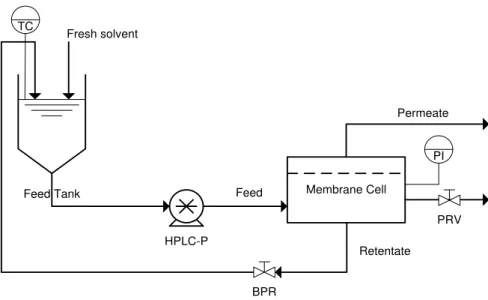
Figure 2.3 Process diagram of the single membrane system (HPLC-P: HPLC pump; BPR:
Back pressure regulator; PRV: Pressure relief valve; PI: Pressure gauge; TC: Temperature controller). ... 36
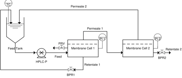
Figure 2.4 Process diagram of the closed loop system. (HPLC-P: HPLC pump; BPR: Back pressure regulator; PRV: Pressure relief valve; PI: Pressure gauge; TC: Temperature controller). ... 37
Figure 3.1 Schematic diagram of the closed-loop membrane process. ... 40
Figure 3.2 Photograph of the feed solution at the beginning (F0, 40 times diluted) and after 8
diafiltration volumes (F8, 8 times diluted) and of the permeate samples at each diafiltration volume (P1-P8, without dilution). ... 45
Figure 3.3 Calculated and experimental mass profiles of product (SY7) and waste (BBR) in (a) feed tank and (b) membrane cell for the purification of model mixture A using single membrane process with a PI2411 membrane disc at 30 bar and 22 °C. Curve fitting was done by assigning different values to : Model 1- / , Model / ; Model 3- / . ... 46
Figure 3.4 Yield and purity profiles for the purification of model mixture A using single membrane process with a PI2411 membrane disc at 30 bar and 22 °C. Curve fitting was done by assigning different values to : Model 1- / , Model / ; Model 3- / . ... 47
Figure 3.5 Calculated and experimental mass profiles of the product (SY7) and waste (BBR)
in (a) feed tank, (b) membrane cell 1 and (c) membrane cell 2 for the purification of model mixture A using the closed-loop membrane process with a PI2411 and a DM150 membrane disc. Curve fitting was done by assigning different values to : Model 1- and , Model 2- and , Model 3- and .. ... 50
Figure 3.6 Yield and purity profiles for the purification of model mixture A using closed-loop
XVII
Figure 3.7 Calculated and experimental mass profiles of the product (SY7) and waste (BBR)
in (a) feed tank and (b) membrane cell 1 after disconnecting the second cell from the system PI24411/DM150 ( ). ... 54
Figure 3.8 Yield and purity profiles for the purification of model mixture A after disconnecting
the second cell from the system PI24411/DM150 ( ). ... 55 Figure 3.9 Calculated and experimental mass profiles of the product (SY7) and waste (BBR) in (a) feed tank, (b) membrane cell 1 and (c) membrane cell 2 for the purification of model mixture A using closed-loop membrane process with a PI2411 and a TFC-MPD discs. Curve fitting was done by assigning different values to : Model 1- / and / , Model 2- / and / , Model 3- / and / .. ... 57
Figure 3.10 Yield and purity profiles for the purification of model mixture A using the closed-loop membrane process with a PI2411 and a TFC-MPD disc Curve fitting was done by assigning different values to : Model 1- / and / , Model 2- / and / , Model 3- / and / .. ... 59
Figure 3.11 Calculated and experimental mass profiles of the product (SY7) and waste (BBR) in (a) feed tank and (b) membrane cell 1 after disconnecting the second cell from the system PI24411/TFC-MPD. Curve fitting was done by assigning different values to : Model 1- / , Model 2- / . ... 61
Figure 3.12 Yield and purity profiles for the purification of model mixture A after
disconnecting the second cell from the system PI24411/TFC-MPD. Curve fitting was done by assigning different values to : Model 1- and , Model 2- and . ... 62
Figure 3.13 Effect of product rejection in the solvent recovery stage in a closed-loop membrane process to the product yield. Simulations were performed assuming that and . ... 64
Figure 3.14 Calculated yield and purity profiles for the purification of model mixture B using
XVIII
Figure 3.15 Flux profiles over time at 10 bar and 27 °C for the membranes screened using
model mixture C. The flux at time 0 is the flux of pure MeOH. ... 73
Figure 3.16 Calculated and experimental mass profiles of product (MY) and waste (BBR) in
(a) feed tank and (b) membrane cell for the purification of model mixture C using single membrane process with a PI2211 disc at 30 bar and 22 °C. ... 78
Figure 3.17 Calculated and experimental concentration profiles in the permeate for the
purification of model mixture C using the single membrane process with a PI2211 disc at 30 bar and 22 °C... 79
Figure 3.18 Photograph of the initial and final feed and of retentate and permeate samples at
each diafiltration volume. Feed and retentate samples were 40 times diluted. ... 79
Figure 3.19 Yield and purity profiles for the purification of model mixture C using single membrane process with a PI2211 disc at 30 bar and 22 °C. ... 80
Figure 3.20 Calculated and experimental mass profiles of the product (MY) and waste (BBR)
in (a) feed tank, (b) membrane cell 1 and (c) membrane cell 2 for the purification of model mixture C using the closed-loop membrane process with a PI2211 and a TFRO-SG disc at 25 °C. Curve fitting was done by assigning different values to the rejections: Model 1- ,/ , and / , Model / and . ... 83
Figure 3.21 Yield and purity profiles for the purification of model mixture C using closed-loop
membrane process with a PI2211 and a TFRO-SG disc at 25 °C. Curve fitting was done by assigning different values to the rejections: Model 1- ,/ , and / , Model 2- / and . ... 84
Figure 3.22 Yield and purity profiles for the purification of model mixture C after
disconnecting the second cell from the system PI2211/TFRO-SG. ... 86
Figure 3.23 Experimental and calculated concentration profiles for the product (MY) and waste (BBR) in the permeate. ... 86
Figure 3.24 Calculated and experimental mass profiles of product (MY) and waste (BBR) in
XIX
assigning different values to and : Model 1- / ; Model 2- / ; Model 3- / . ... 89
Figure 3.25 Yield and purity profiles for the purification of model mixture C using single membrane process with a PBI 24xDBX disc at 21 bar and 23 °C. Curve fitting was done by assigning different values to and : Model 1- / ; Model 2- / ; Model 3- / . ... 90
Figure 3.26 Experimental and calculated concentration profiles for the product (MY) and
waste (BBR) in the permeate. Curve fitting was done by assigning different values to and : Model 1- / ; Model 2- / ; Model 3- / . ... 91
Figure 3.27 Calculated and experimental mass profiles of the product (MY) and waste (BBR)
in (a) feed tank, (b) membrane cell 1 and (c) membrane cell 2 for the purification of model mixture C using closed-loop membrane process with a PBI 24xDBX and a PBI 26xDBB disc. Curve fitting was done by assigning different values to and : Model 1- , , and ; Model 2- and , and . ... 93
Figure 3.28 Yield and purity profiles for the purification of model mixture C using closed-loop membrane process with a PI2211 and a TFRO-SG disc. Curve fitting was done by assigning different values to and : Model 1- , , and ; Model 2- and , and .. ... 94
Figure 3.29 Yield and purity profiles for the purification of model mixture C after
disconnecting the second cell from the system PBI 24xDBX/PBI 26xDBB. Curve fitting was done by assigning different values to and : Model 1- / ; Model 2- / ; ... 95
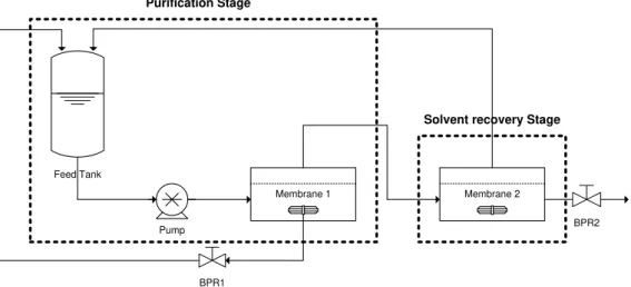
Figure 4.1 Schematic representation of the closed-loop membrane process integrating a cascade of n membrane units for purification. ... 97
Figure 4.2 Flux profiles over time at 10 bar and 25°C for the membranes screened using
model mixture D1. The flux at time 0 is the flux of pure MeCN. ... 100
XX
Figure 4.4 Flux profiles over time at 10 bar and 25°C for the membranes screened using
model mixture D2. The flux at time 0 is the flux of pure MeCN. ... 102
Figure 4.5 Experimental and calculated mass profiles for the polymer (product) and monomer
(waste) using the single membrane process with a PI2341 membrane at 10-15 bar and 21 °C. Calculated curves were obtained considering the an average of the calculated rejections, and . (Model 1) and corrected values, and . (Model 2). ... 105
Figure 4.6 Yield and purity profiles as a function of the number of membrane units used for
XXI
LIST OF TABLES
Table 1.1 Classification of membrane processes according to their driving forces (Mulder,
1996). ... 5
Table 1.2 Comparison of various pressure driven membrane processes. Adapted from (Mulder, 1996). ... 6
Table 1.3 Comparison of solvent use at GSK based on overall manufacturing operations (1995-2000) and more recent pilot plant operations (2005) (Constable, Jimenez-Gonzalez & Henderson, 2007). ... 17
Table 2.1 Properties of the dyes used as model compounds. ... 29
Table 2.2 Summary of the membranes not prepared but used in this work ... 30
Table 2.3 Summary of the integrally skinned PI membranes prepared... 31
Table 2.4 Summary of the integrally skinned PBI membranes prepared. ... 32
Table 2.5 Summary of the TFC membranes prepared. ... 33
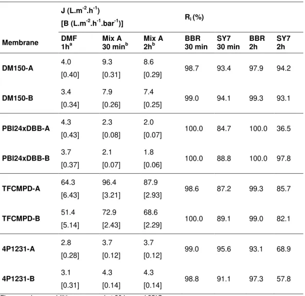
Table 3.1 Summary of the screening results for 14 cm2 membrane discs using model mixture A (Mix A). ... 43
Table 3.2 Summary of the data recorded during the diafiltration of model mixture A using the single membrane process with a PI2411 membrane disc. ... 44
Table 3.3 Summary of the data recorded along the diafiltration of model mixture A using the closed-loop membrane process with a PI2411 membrane disc for purification and a DM150 membrane disc for solvent recovery. ... 49
Table 3.4 Summary of the data recorded along the diafiltration of model mixture A using the single membrane process with a PI2411 membrane disc after disconnected the cells. ... 53
XXII
Table 3.6 Summary of the data recorded along the diafiltration of model mixture A using the
single membrane process with a PI2411 membrane disc after disconnected the cells. ... 60
Table 3.7 Comparison between the three processes used to purify model mixture A. ... 63
Table 3.8 Summary of the screening data. ... 67
Table 3.9 Physical parameters of the solvents. ... 74
Table 3.10 Rejections after 5h and 24h of operation at 10 bar and 27°C for the membranes
screened using model mixture C. ... 74
Table 3.11 Summary of the data recorded along the diafiltration of model mixture C using the single membrane process with a PI2211 membrane. ... 77
Table 3.12 Summary of the data recorded along the purification of model mixture C using the
closed-loop membrane process with a PI2211 membrane disc for purification and a TFRO-SG membrane disc for solvent recovery. ... 81
Table 3.13 Summary of the data recorded along the purification of model mixture C using the single membrane process with a PI2211 membrane disc after disconnecting the second cell from the system. ... 85
Table 3.14 Comparison between the performance of the single membrane process with
PI2211 membrane and the closed-loop membrane process with PI2211 and TFRO-SG membranes. ... 87
Table 3.15 Summary of the data recorded along the purification of model mixture C using the single membrane process with a PBI 24xDBX membrane. ... 88
Table 3.16 Summary of the data recorded along the purification of model mixture C using the closed-loop membrane process with a PBI 24xDBX membrane disc for purification and a PBI 26xDBB membrane disc for solvent recovery. ... 92
Table 3.17 Summary of the data recorded along the diafiltration of model mixture C using the
single membrane process with a PBI 24xDBX membrane disc after disconnected the cells. .... 95
XXIII
Table 4.1 Rejections after 2h of operation at 10 bar and 25 °C for the different membranes
tested against model mixture D2. ... 103
Table 4.2 Performance data for the purification of the product crude using PI2341 membrane
at 21 °C. ... 104
XXV
ABREVIATIONS
API(s) Active pharmaceutical Ingredient(s) BBR Brilliant Blue R
BPR Back pressure regulator DBB Dibromobutane
DBX Dibroxylene
DMAc N,N-dimetylacetamide (DMAc) DMF N,N-dimethylformamide GHGs Green house gases
HDA 1,6-Hexanediamine
HPLC High pressure liquid chromatography IPA Isopropanol
MeCN Acetonitrile MeOH Methanol
MF Microfiltration
MPD m-phenylene diamine MW Molecular weight (g.mol-1) MWCO Molecular weight cut-off
MY Martius Yellow NF Nanofiltration
OSN Organic solvent nanofiltration
PA Polyamide
PBI Polybenzimidazole PEEK Poly(ether ether ketone)
PEG Polyethylene glycol PI Polyimide
PP Polypropylene PRV Pressure relief valve
PS Polystyrene RO Reverse Osmosis
SRNF Solvent resistant nanofiltration SY7 Solven Yellow 7
TFC Thin-film composite THF Tetrahudrofuran
UF Ultrafiltration UV Ultraviolet
XXVI
NOMENCLATURE
Fraction in the retentate (dimensionless) Fraction in the permeate (dimensionless) Rejection of solute (%)
Concentration (g.L-1) Pressure (bar) Temperature ( ) Solute flux (g.m-2.h-1) Solvent flux (L.m-2.h-1)
Hydrodynamic permeability (L.m-2.h-1.bar-1)
̅ Logarithmic average of solute concentration across the membrane (g.L-1) Radius (m)
Solute hindrance factor for convection (dimensionless) Solvent velocity (m.s-1)
Faraday constant (96487 C.mol-1) Gas constant (8.341 J.mol-1.K-1)
Corrected diffusive coefficient according to (Bowen & Welfoot, 2002) (m2.s-1) Valence (dimensionless)
Fick’s aw diffusiv c ffici t (m2.s-1) Sorption coefficient (dimensionless) Membrane thickness (m)
Concentration of the solute in the feed side (mol.m-3) Concentration of solute in the permeate side (mol.m-3)
Membrane area (m2)
Solvent permeability ((L.m-2.h-1.bar-1) Volume (L)
Time (h)
Number of diafiltration volumes (dimensionless) Mass (g)
Yield of product (%) Purity of product (%)
XXVII
GREEK SYMBOLS
Separation factor (dimensionless) Reflection coefficient (dimensionless) Osmotic pressure (bar)
Osmotic permeability (g.m-2.h-1.bar-1) Surface porosity (dimensionless) Pore tortuosity (dimensionless) Solvent viscosity (kg.m-1.s-1) Partial molar volume (m3.mol-1) Electrical potential (V)
Boundary layer thickness (m)
Maximum absorbance wavelength (nm)
SUBSCRIPTS
Species/Ion Volume Solute
Membrane surface Bulk
P Permeate side
R Retentate side
F Feed side
Limiting
1
Chapter 1
Literature Review
1.1. MEMBRANE TECHNOLOGY
1.1.1. The Membrane
There are many membrane processes based on different separation principles or mechanisms. However, in spite of these various differences, all membrane processes have one thing in common: the membrane. A membrane can be considered as a selective barrier between two phases, allowing only some components to pass through (Mulder, 1996).
A schematic representation of a two-phase system separated by a membrane is presented in Figure 1.1. The separation is achieved because the membrane has the ability to transport one component from the feed to the permeate side more readily than any other component. The transport trough the membrane takes place as a result of a driving force, i.e. a chemical or electrical potential difference, acting on the components in the feed. Either pressure ( ), concentration ( ) or temperature ( ) differences contribute to the chemical potential difference of a component (Mulder, 1996).
Membrane
Phase 1/
Feed
Phase 2/
Permeate
Driving Force
ΔC, ΔP, ΔT, ΔE
Component 1
Component 2
2
1.1.2. Membrane types
Synthetic membranes can be organic (polymeric or liquid) or inorganic (ceramic, metal or zeolite) (Mulder, 1996).
Polymeric membranes are commonly classified according to its structure as symmetric or asymmetric. These two classes can be subdivided as shown in Figure 1.2.
Asymmetric Membranes
Porous membrane Nonporous/Dense membrane
Integrally Skinned membrane Thin Film Composite membrane
Symmetric Membranes
Figure 1.2 Principal types of membranes. Adapted from (Baker, 2004, Mulder, 1996).
Symmetric membranes consist of a porous or dense (nonporous) polymer layer with a thickness ranging roughly from 10 to 200 μm. The resistance to mass transfer is determined by the total membrane thickness, whether the membrane is porous or dense (Mulder, 1996). However, in the first case the separation is mainly a function of molecular size and pore distribution, whereas in the second case it is a function of the diffusivity and solubility of the molecules in the membrane material. When these membranes are charged, they mostly separate by exclusion of ions of the same charge as the fixed ions of the membrane structure (Baker, 2004).
3 can be separately optimized (Baker, 2004, Mulder, 1996). The most used methods for asymmetric membrane preparation will be explained in greater detail insection 1.1.3.
The interest in membranes formed from less conventional materials has increased. Ceramic membranes, the main class of inorganic membranes, are being fairly applied in microfiltration and ultrafiltration fields, since these membranes possess superior chemical, thermal and structural stability relative to polymeric membranes. They do not deform under pressure, do not swell and are cleaned easily, since all kinds of cleaning agents, such as strong acids and alkali, can be used. Furthermore, they have a greater lifetime than that of organic polymeric membranes. However, they tend to be more expensive and brittle than polymeric membranes and are also less versatile in applications. In addition, their large-scale synthesis and module construction is not as easy as for polymeric membranes(Vandezande, Gevers & Vankelecom, 2008). That is why the majority of membranes used commercially are still polymer-based (Vandezande, Gevers & Vankelecom, 2008, Baker, 2004, Mulder, 1996).
1.1.3. Membrane preparation techniques
There are a number of membrane preparation techniques. The kind of technique employed depends mainly on the material used, despite some techniques can be used to prepare both polymeric and inorganic membranes, and on the desired membrane structure, which in turn is dependent on the separation problem. The most important techniques are sintering, stretching, track-etching, phase inversion, sol-gel process, vapour deposition and solution coating. With the first three techniques only porous membranes are obtained. These membranes can also be used as sublayer for composite membranes. Through the use of phase inversion techniques it is possible to obtain open as well as dense structures (Mulder, 1996).
The basic support material for a composite membrane is often an asymmetric membrane obtained by phase inversion. The separating layer can be prepared via dip-coating, spray coating, spin coating, interfacial polymerisation, in-situ polymerisation, plasma polymerisation and grafting. Except for the first three methods, all the techniques involve polymerisation reactions which generate new polymers as a very thin layer (Mulder, 1996).
Preparation techniques for both phase inversion membranes and for composite membranes by interfacial polymerisation will be described hereafter.
1.1.3.1. Phase inversion
Most commercially membranes are obtained by phase inversion since this represents one of the most versatile, economical and reproducible formation mechanisms for polymeric asymmetric membranes (Vandezande, Gevers & Vankelecom, 2008) (Mulder, 1996).
-4 s a at s” i t a -rich and a polymer lean-phase, ultimately forming the matrix and the pores of the membrane, respectively. This phase separation can be induced by immersing the film in a non-s v t bath (“i si ci itati ”) b w i g th t atu (“th a ci itati ”) b va ati g th v ati s v t f th fi (“c t d va ati ”) b aci g th cast fi i a -solvent vapour phas (“ ci itati f th va u has ”) Th st c has i v si th d is has i v si I this case the phase separation occurs because of the exchange of solvent and nonsolvent. When th d ixi g sta ts di ct (“i sta ta us d ixi g”) and the membrane forms immediately after immersion in the nonsolvent bath, a porous membrane structure will develop. On the other ha d wh th d ixi g tak s s ti b f th b a is f d (“d a d d ixi g”) a b a with a atively dense top layer is obtained. A phenomenon often associated with immersion-precipitation, mostly with instantaneous precipitation, is the formation of macrovoids. These are enlongated, finger- or tear-like pores that can extent over the entire membrane thickness. They are generally considered undesirable as they cause mechanically weak spots in the membrane and thus severely limit the compaction resistance. Conditions favouring delayed demixing however can reduce or even suppress macrovoid formation, e.g. by adding a volatile co-solvent to the casting solution, by increasing the polymer concentration in the casting solution, by selecting a non-solvent with limited miscibility with the solvent in the casting solution, or by introducing an evaporation step before immersion of the cast film into the coagulation bath (Vandezande, Gevers & Vankelecom, 2008, Mulder, 1996).
In order to increase the separation performance of asymmetric membranes and to increase their long-term stability, several post-treatment or conditioning procedures can be used, such as annealing (wet or dry), crosslinking (chemical, plasma or photo-induced), drying by solvent exchange and treatment with conditioning agents, such as lube oils, glycerol or long chain hydrocarbons (Vandezande, Gevers & Vankelecom, 2008).
1.1.3.2. Interfacial polymerization
Interfacial polymerization has become a well-established and useful technique to prepare the dense, active top-layer of TFC membranes. The technique entails the application of an ultra-thin film upon an asymmetric, porous support-layer (normally prepared by phase inversion), via an in-situ polymerization reaction occurring at the interface between two immiscible solvents containing reactive monomers (Vandezande, Gevers & Vankelecom, 2008).
First, the support is impregnated, typically with an aqueous diamine solution. Then, and after remove the excess water, the saturated support is contacted with an organic phase containing acyl halides. Both monomers then react with each other and quickly form a thin selective polyamide layer that remains attached to the substrate. As soon as the top-layer is formed, it acts as a barrier for further monomer transport thus controlling the top layer thickness (Vandezande, Gevers & Vankelecom, 2008).
5 partition coefficients and reactivities, possible additives, solubility of the nascent polymer in the solvent phase, overall kinetics and diffusion rates of the reactants, presence of by products, competitive side reactions, crosslinking reactions and post reaction treatment. Higher monomer concentrations, higher reaction rates and longer polymerization times generally improve the efficiency of film formation. This results in thicker and denser barrier-layers with increased rejections but decreased fluxes (Vandezande, Gevers & Vankelecom, 2008).
The performance of TFC membranes can be further enhanced by applying an adequate post-polymerization treatment. Different techniques have been described including grafting, curing, plasma, UV and chemical treatment (Vandezande, Gevers & Vankelecom, 2008).
1.1.4. Membrane processes
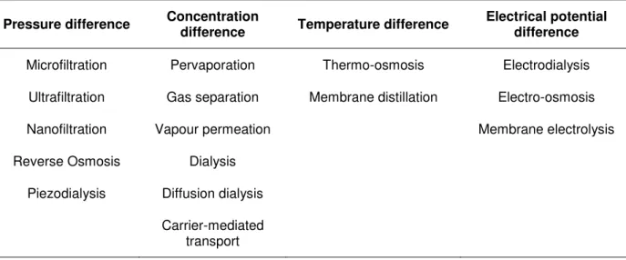
Membrane processes can be classified according to their driving forces - Table 1.1
Table 1.1 Classification of membrane processes according to their driving forces (Mulder, 1996).
Pressure difference Concentration
difference Temperature difference
Electrical potential difference
Microfiltration Pervaporation Thermo-osmosis Electrodialysis Ultrafiltration Gas separation Membrane distillation Electro-osmosis
Nanofiltration Vapour permeation Membrane electrolysis
Reverse Osmosis Dialysis Piezodialysis Diffusion dialysis
Carrier-mediated transport
The most important pressure driven membrane processes are microfiltration (MF), ultrafiltration (UF), nanofiltration (NF) and reverse osmosis (RO). All of them are used to concentrate or purify a dilute (aqueous or non-aqueous) solution. What differs between them is basically the size of the solutes to be separated. As we go from microfiltration trough ultrafiltration and nanofiltration to reverse osmosis, the size (or molecular weight) of the particles or molecules separated diminishes and consequently the pore size in the membrane become smaller. This also implies that the resistance of the membranes to mass transfer increases. That is why higher pressures are applied when we go from microfiltration to reverse osmosis (Mulder, 1996). A comparison of the various pressure driven processes is given in
Table 1.2.
6 polymeric and ceramic, that can function in organic solvents. With those membranes a new technology, commonly designated by organic solvent nanofiltration (OSN) or solvent resistant nanofiltration (SRNF), has born, opening new opportunities in the chemical and refining industries (Boam & Nozari, 2006, White, 2006). Processes involving OSN membranes were already proposed for edible oil deacidification (Rama, Cheryan & Rajagopalan, 1996), lube oil dewaxing (White & Nitsch, 2000), solvent exchange (eg. exchanging a high boiling point solvent, such as toluene, for a low boiling point solvent, like methanol (Lin & Livingston, 2007), solvent recovery (see section 1.2.3), homogeneous (Luthra et al., 2002) and phase transfer catalysts (Luthra et al., 2001) reuse or recycling, product purification (e.g separation of amino acids (Reddy et al., 1996) or antibiotics from organic solvents (Shi et al., 2006)) and enantiomer separation (Ghazali et al., 2006).
Table 1.2 Comparison of various pressure driven membrane processes. Adapted from (Mulder, 1996).
Microfiltration Ultrafiltration Nanofiltration/ Reverse Osmosis
Separation of particles Separation of macromolecules
(bacteria, yeasts) Separation of low MW solutes (salts, glucose, lactose, micropollutents)
Pore sizes ≈ 0,05-10 μm Pore sizes ≈ 1-100 nm Pore sizes ˂ 2nm Applied pressure low (˂ 2
bar) Applied pressure low (1-10 bar) Applied pressure high (≈ 10-60 bar) Separation based on the
particle size Separation based on the particle size Separation differences on solubility and based on diffusivity
Gas separation and pervaporation are two important concentration driven membrane processes. The first one is actually the only concentration driven process for which was reported the utilization of both porous and dense membranes. All the other require the utilization of a dense membrane (asymmetric and/or composite membrane). It is a process used, not only for the separation of different gaseous mixtures (e.g. H2/He, CH4/CO2, O2/N2), including isotopic mixtures, but also for the dehydration (drying) of gases, and for the separation of organic vapours from non-condensable gases. Pervaporation, by its turn, is the only membrane process where phase transition occurs, with the feed being a liquid and the permeate a vapour. This process is generally used to separate a small amount of liquid from a liquid mixture and it is particularly attractive when the liquid mixture exhibits an azeotropic composition (Mulder, 1996).
7 difference between feed and permeate. This process is mainly applied to the production of pure water and removal of volatile organic compounds (Mulder, 1996).
Membrane processes such as electrodialysis, in which the driving force is supplied by an electrical potential difference, can only be employed when charged molecules are present using ionic or charged membranes. This process is used on the desalination of water, production of salt and separation of amino acids (Mulder, 1996).
1.1.5. Membrane characterization
Membranes can be characterized in terms of its performance or morphology. The most important performance related parameters are flux, permeability, rejection, diffusion coefficients and separation factors. Morphological parameters include both physical (e.g. pore shape, pore size, pore distribution, membrane/top layer thickness), and chemical parameters (e.g. charge, hydrophobicity). Performance parameters are derived from one or more morphological parameters. However, and despite the importance of characterize and better understand physical-chemical parameters, it is the functional parameters that, from a practical perspective, determine the usefulness of the membrane (Mulherkar & van Reis, 2004, Cuperus & Smolders, 1991).
Normally membrane selection is often based upon two performance parameters which are flux and selectivity. The flux, (L.m-2.h-1), also denoted by permeate rate, is defined as the volume of liquid permeating through the membrane per unit area and per unit time. Many parameters like temperature, pressure and solute concentration affect the flux of OSN membranes. The permeate rate tend to increase with increasing temperature, because of reduction in solvent viscosity and increased polymer chain mobility (Van der Bruggen, Geens & Vandecasteele, 2002). An increase in pressure also led to an increase in flux. Solute concentration has an adverse effect on flux because of osmotic pressure and concentration polarisation. The effect of these last two parameters on the flux can be better understood by reading through sections 1.1.6 and 1.1.7.
In turn, the selectivity can be expressed using rejections or separation factors. The rejection towards a solute , (%), is more conveniently used to express the selectivity for mixtures consisting of a solvent and one or more solutes, and is given by
( )
1-1
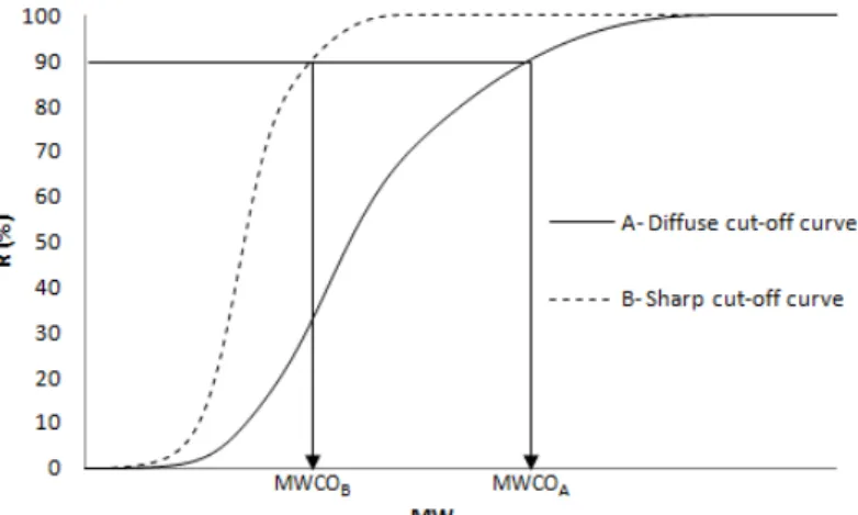
8 By plotting the rejection for different solutes against its molecular weights (rejection or cut-off curve) it is ssib t d iv th ‘ cu a w ight cut- ff’ ( WCO) f th b a which represents the molecular weight (MW) of a reference compound that is typically 90% rejected by the membrane. NF and OSN membranes are characterised by a sigmoidal rejection curve, as the ones depicted in Figure 1.3, and a MWCO between 200-1000 (Vandezande, Gevers & Vankelecom, 2008, Mulder, 1996).
Figure 1.3 Typical rejection curves for membranes with a A) sharp off and a B) diffuse cut-off. Adapted from (Mulder, 1996).
The MWCO is particular useful when the mixture to be separated contains more than one component and all of different sizes. It should be noted, however, that MWCO itself can be a poor estimation of membrane performance, as the pore size distribution, solvent environment, molecular shape, charge, functional groups, occurrence of polarisation phenomena, temperature and the applied pressure also affect rejection. Nevertheless, the MWCO is still a good starting point when screening for suitable membranes (Kim, 2011, Vandezande, Gevers & Vankelecom, 2008, See Toh et al., 2007, Yang, Livingston & Freitas dos Santos, 2001, Mulder, 1996).
For gas mixtures and mixtures of organic solvents the selectivity is usually expressed in terms of the separation factor, α. For a mixture consisting of two components A and B the separation factor αA/B is given by
⁄
⁄ 1-2
9
1.1.6. Transport in membranes
It is possible to distinguish three groups of mathematical models that describe transport through membranes. One group of models originates from irreversible thermodynamics, treating the membrane as a black-box; the other two, the pore-flow and the solution diffusion models, take into account membrane properties (Vandezande, Gevers & Vankelecom, 2008).
One of the models based on irreversible thermodynamics was derived by Kedem & Katchalsky (1958). They proposed the following equations for the volume flux, , and the solute flux, , through a membrane:
1-3
̅ 1-4
where is the hydrodynamic permeability, is the hydrodynamic pressure difference across the membrane, is the reflection coefficient ( ), which can be interpreted as the fraction of solute reflected by the membrane in convective flow (Vandezande, Gevers & Vankelecom, 2008), is the osmotic pressure difference across the membrane, ̅ is the logarithmic average of solute concentration across the membrane and is the osmotic (solute) permeability. This kind of mathematical models have some limitations, since they do not take into account any information related to the nature or structure of the membrane. However, they not only allow for a very clearly description of the fluxes but also predict the existence of coupling of driving forces: equation 1-3 shows that even if there is no difference in hydrodynamic pressure across the membrane ( ) there is still a volume flux; on the other hand, equation 1-4 indicate that if the solute concentration on both sides of the membrane is the same ( ) there is still a solute flux when (Mulder, 1996).
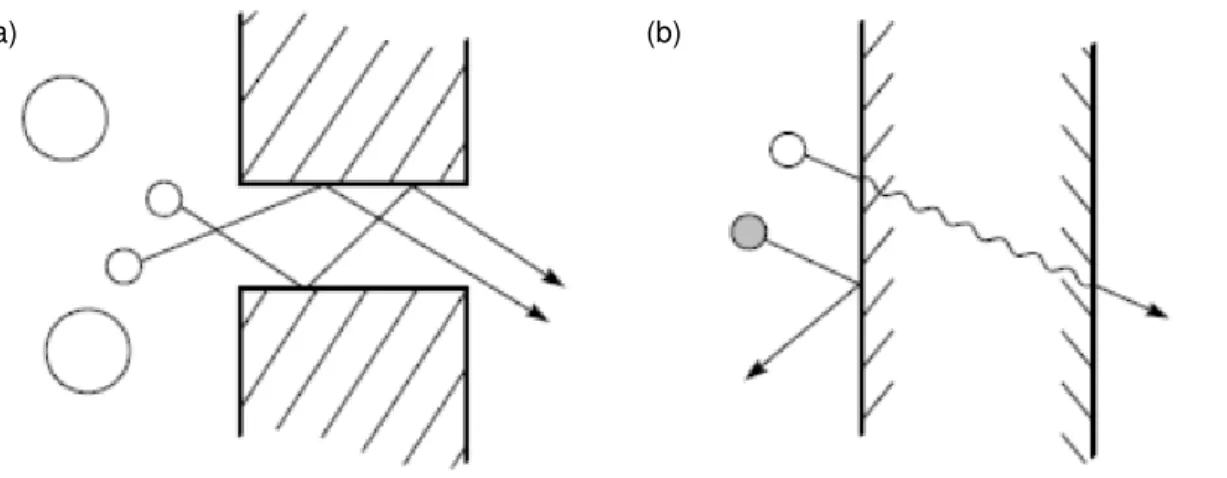
The most reliable transport models are the pore-flow and the solution-diffusion models. They are used to describe, respectively, the transport through porous (e.g. micro and ultrafiltration membranes) and dense membranes (e.g. reverse osmosis, gas separation and pervaporation membranes).
According to the pore-flow model, there is no solute or solvent concentration gradients over the membrane and the permeants are transported by pressure-driven convective flow through tiny pores. Separation occurs because one of the permeants is excluded (filtered) from some of the pores in the membrane through which other permeants move (see Figure 1.4-a). Like this, the volume flux through the pores may be described by the Hagen-Poiseuille equation:
10 where is the surface porosity, is the pore radius, is the pore tortuosity, is the solvent viscosity, and ⁄ is the pressure gradient over the membrane (Vandezande, Gevers & Vankelecom, 2008, Baker, 2004).
(a) (b)
Figure 1.4 Schematic representation of the most important transport mechanisms through membranes: (a) the pore-flow model and (b) the solution-diffusion model (Baker, 2004).
For the solute flux, several empirical pore-flow models have been developed. Bowen et al. proposed a model based on the hydrodynamic model proposed by Ferry (1936), to describe the transport of uncharged solutes, and another one, based on the extended Nernst-Plank equation, to describe the transport of charged solutes (Bowen & Welfoot, 2002). Both models were modified to include the hindered convection and diffusion within the pores as proposed by Deen (1987):
1-6
1-7
where and are the solute and ionic hindrance factors for convection, and are the partial molar volume of the solute and ion, is the valence of the ion, and are the solute and ion concentrations within pore, is the solvent velocity, ⁄ and ⁄ are the concentration gradient of the solute and ion over the membrane, ⁄ is the electrical potential gradient over the membrane, is the absolute temperature, is the Faraday constant and is the gas constant, and and are the solute and ion pore diffusion coefficients, corrected for the diffusive hindrance and for the change in solvent viscosity with pore radius.
11 (Baker, 2004). Following the assumptions made, two simple equations could be derived for volume and solute flux:
1-8
( ) ( ) 1-9
where and a th Fick’s aw diffusi c fficients, and are the solvent sorption and the solute distribution, respectively, is the solvent concentration, is the solvent molar flux, is the membrane thickness, is the solute concentration in the feed side and is the solute concentration in the permeate side; the constants and are known as the solvent and solute permeability, respectively. According to equation 1-8 the solvent flux through a membrane remains small up to the osmotic pressure of the solute solution and then increases with applied pressure, whereas according to equation 1-9 the solute flux is essentially independent of the pressure. This explains why the rejection may increase with applied pressure for RO processes (Baker, 2004).
OSN membranes are intermediate between truly porous and truly solution-diffusion membranes, and so they are best described by transient mechanisms that take into account the changing contributions of the diffusive and convective mechanisms, like the irreversible thermodynamics and the pore-flow models presented, or the solution-diffusion with imperfections model (Bhanushali, Kloos & Bhattacharyya, 2002, Mason & Lonsdale, 1990), that accounts for the occurrence of convective flow and for the partial flux coupling effect. Plus, and since OSN membranes are applied to non-aqueous systems, special considerations regarding the various interactions between the system components and membrane swelling are also needed (Boam & Nozari, 2006, Dijkstra, Bach & Ebert, 2006, Robinson et al., 2004, Bhanushali, Kloos & Bhattacharyya, 2002).
1.1.7. Strengths and limitations of membrane processes
12 In spite of all these advantages, and after all the progress in this area, membrane processes still have some limitations, that particularly slow down large-scale applications (Van der Bruggen, Mänttäri & Nyström, 2008, Baker, 2006). The most relevant limitations are discussed in the following sub-sections. A special attention was given to problems related to pressure driven membrane processes, like NF and OSN.
1.1.7.1. Concentration polarization and membrane fouling
Concentration polarization is basically the formation of concentration gradients due to differences in the permeate rates of the feed mixture components. By convention, concentration polarization effects are described by considering the concentration gradient(s) of the minor component(s), which can be the more or the less retained component(s), depending on the process. Plus, since in most membrane processes there is a bulk flow of a liquid or a gas through the membrane, only concentration gradients formed on the feed side are considered (Baker, 2004).
Pressure driven processes, like MF, UF, NF and RO, are usually applied to solutions consisting of a solvent, that can permeate through the membrane more or less freely, and one or more solutes, that are retained to different extents by the membrane. The retained solute(s) can accumulate at the membrane surface where their concentration will gradually increase. This causes not only a reduction in the driving force for the solvent, that translates in a flux decline, but also an increase in the driving force for the solute(s), reducing membrane selectivity. The increase in solute concentration at the membrane surface can also lead to a diffusive back flow towards the bulk of the feed, resulting in a concentration gradient between the bulk ( ) and the membrane surface ( ) – boundary layer-, like the one depicted in Figure 1.5, which increases the resistance to mass transfer (Mulder, 1996).
Bulk feed Boundary layer Membrane
cs,b
cs,m
cs,p
x δ 0
Figure 1.5 Concentration polarization: concentration profile under steady-state conditions.
13 surface, by using membrane spacers, or by using pulsating flow, as all these options increase turbulent mixing at the membrane surface. However, the energy consumption of the pumps required and the pressure drops produced imposes a practical limit to the turbulence that can be obtained in a membrane module (Baker, 2004, Mulder, 1996).
It is known that concentration polarization increases exponentially with the volume flux, . That is why after a certain pressure, the flux does not increase further on increasing the pressure and the so called limiting flux, , is achieved (see Figure 1.6). Thus, there is no point in having super-high-flux membranes, since the maximum flux will always be limited by osmotic pressure and concentration polarization. The only advantage of these membranes would be a reduction in energy costs, since they would allow for the same flux at lower applied pressure, minimize the overall processing time and limit the required membrane area (Baker, 2004).
ΔP Jv Pure water
Solution J∞
Figure 1.6 Flux as a function of the applied pressure both for pure water and for a solution: the flux of pure water increases lineary with applied pressure, considering that no compaction occurs; however when solutes are added to water the flux starts platteauing after a certain applied pressure (Mulder, 1996).
In the worst case scenario concentration polarisation can result in membrane fouling, which is the deposition of retained solutes in the membrane, by adsorption, pore blocking, precipitation or cake formation. The type of separation problem and the type of membrane used in MF and UF make these processes the most susceptible to concentration polarization and fouling of all pressure driven membrane processes (Mulder, 1996). Fouling problems are, however, much more complex for NF processes, since the interactions leading to fouling take place at nanoscale, and are therefore difficult to understand (Van der Bruggen, Mänttäri & Nyström, 2008).
One of the main consequences of membrane fouling (and concentration polarization) is the decrease of flux. This has a negative impact on the operational costs of the process, since the permeate production gets lower and/or higher transmembrane pressures are required (Mulder, 1996).
14 would allow to virtually abolish the problem (Van der Bruggen, Mänttäri & Nyström, 2008, Mulder, 1996).
1.1.7.2. Insufficient separation
The incompleteness of the separation is a major impediment for a wide application of membrane processes, including NF (Van der Bruggen, Mänttäri & Nyström, 2008).
As described in sub-section 1.1.5, NF membranes are characterized by a sigmoidal rejection curve, which is never completely sharp. This results in an insufficient separation between different compounds on the basis of molecular size. Since the separation depends also on other physical and chemical properties of the compounds/membrane, like charge (Bellona & Drewes, 2005), and since the pores of NF membranes follow a distribution of sizes (Richard Bowen & Doneva, 2000), permeate usually contains molecules with variable sizes, both below and above the claimed average pore size of the membrane. The separation can be even more challenging for OSN processes, since solvents can change membrane characteristics, like pore size and hydrophobicity (Van der Bruggen, Geens & Vandecasteele, 2002), and even solute characteristics, like solute effective diameter (Geens et al., 2005). Therefore, a single membrane separation is often insufficient to obtain the desired separation (Van der Bruggen, Mänttäri & Nyström, 2008).
There are different process strategies to overcome this problem, like multiple membrane passages, diafiltration or membrane cascades. As will be seen in section 1.3, membrane cascades offer further benefits, and begin to be considered for NF and OSN processes (Van der Bruggen, Mänttäri & Nyström, 2008).
1.1.7.3. Membrane compaction
Compaction is the mechanical deformation of a polymeric membrane matrix, due to the sealing and collapse of the pores at elevated pressures. Thus, this is a phenomenon which occurs specially with porous membranes used in pressure driven membrane operations, where the applied pressures are relatively high, like NF and RO (See Toh, Silva & Livingston, 2008, Mulder, 1996). However, dense membranes tend also to suffer some compaction when exposed to swelling conditions (Vankelecom et al., 2004). This is never a problem for ceramic membranes due to their superior mechanical stability.
15
1.1.7.4. Low membrane stability and lifetime
In the case of NF and OSN processes, membrane stability and lifetime is related to the occurrence of fouling (and therefore, the need for cleaning), and the application of membranes in demanding circumstances, such as the ones created by organic solvents (Van der Bruggen, Mänttäri & Nyström, 2008).
For aqueous applications, membrane lifetime depends on the overall strategy against membrane fouling. Applications where fouling requires frequent cleaning often face a faster membrane deteoration, because even the mildest cleaning agents damage the membrane to some extent (Van der Bruggen, Mänttäri & Nyström, 2008).
In the case of OSN, membrane lifetime depends mostly on the compatibility between the membrane and the solvents. Recurrent problems resulting from the interaction between polymeric membranes and organic solvents are swelling, deformation or (ultimately) dissolution of the membrane (Van der Bruggen, Mänttäri & Nyström, 2008).
16
1.2. SOLVENT USE IN THE PHARMACEUTICAL INDUSTRY
1.2.1. Solvent utilization
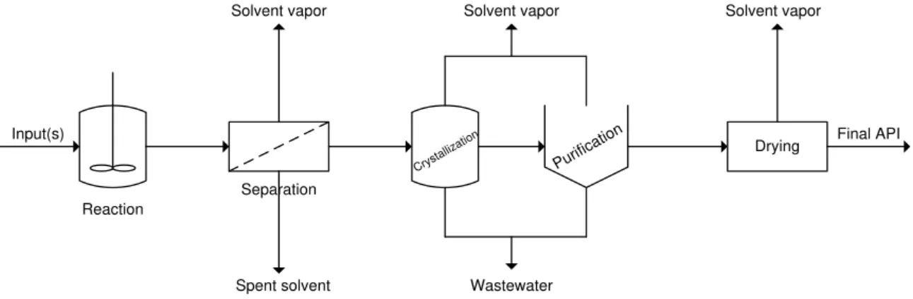
The manufacturing of a drug product involves two phases: 1) the production of the active pharmaceutical product (API) and 2) the formulation process, in which the API is combined with one or more excipients to produce the final product. During all the manufacturing process, solvents are inevitably used for cleaning process equipment and for analytical instruments employed for process control and quality assurance. However, during the batch-wise API synthesis phase solvents are used for many other purposes (Dunn, Wells & Williams, 2010).
Most APIs are produced using liquid phase organic reactions which often require large quantities of different solvents. Between each reaction step, there are a series of operations required to separate, purify and isolate APIs intermediates (work-up phase), that frequently require more solvents and/or generate solvent wastes. Because of the considerable number of steps and the large amount of solvents required per each step, solvent use can account for as much as 80-90% of the total mass in an API production process (Dunn, Wells & Williams, 2010). A scheme of the different steps involved in a typical API synthesis process, including solvent waste streams generated in each step is shown on Figure 1.7.
Reaction
Separation
Drying Input(s)
Spent solvent Solvent vapor
Final API
Wastewater
Solvent vapor Solvent vapor
Crystall
ization
Purifica tion
Figure 1.7 Typical pharmaceutical batch operation. Adapted from (Dunn, Wells & Williams, 2010).
17 Table 1.3 Comparison of solvent use at GSK based on overall manufacturing operations (1995-2000) and more recent pilot plant operations (2005) (Constable, Jimenez-Gonzalez & Henderson, 2007).
Chemical GSK pilot plant processes (2005 rank)
GSK manufacturing processes (1995-2000 rank)
2-Propanol 1 5
Ethyl acetate 2 4
Methanol 3 6
Denaturated ethanol 4 8
n-Heptane 5 12
Tetrahydrofuran 6 2
Toluene 7 1
Dichloromethane 8 3
Acetic acid 9 11
Acetonitrile 10 14
Besides all the environmental, health and safety impacts, there are also economical issues that should drive pharmaceutical companies to reduce solvent waste and usage, like the price of purchasing and the price of waste treatment. Purchasing excessive solvent increases raw material costs as well as waste treatment costs for the disposal of these solvents. The cost to purchase fresh solvents varies on the method of transport, the quantity purchased, and the cost of manufacture (Dunn, Wells & Williams, 2010). On the other hand, it is known that 10-35% of the total plant investment can be consumed during the handling, storage and treatment of waste streams (Mulholland & Dyer, 2001).
It is peremptory: if pharmaceutical companies want to contribute to the reduction of the overall environmental footprint, produce efficient and robust processes, and be competitive they will need to minimize solvent utilization and waste generation (Dunn, Wells & Williams, 2010).
1.2.2. Waste minimization and solvent recovery
18 excess. In these situations the only way to avoid or minimize the costs and environmental burden related to solvents usage is by reusing them (Dunn, Wells & Williams, 2010).
Pharmaceutical companies already do their recovery since decades, but they are still seeking ways for enhance the feasibility of solvent recovery processes (Thomas, 2012), by minimizing the input of energy required and/or the waste produced by their own (Dunn, Wells & Williams, 2010).
The capital investment for solvent recovery typically includes piping, tank farms and recovery equipment, which is easy to justify for large volumes and expensive solvents, but not so easy with smaller streams, that ca ’t c ssa i b pooled with other solvents. Thus, there is also a need to find new and integrated ways for solvent recovery (Thomas, 2012).
Currently, distillation is used for approximately 95% of all solvent separation processes. However it leads to waste generation, such as the release of green house gases (GHGs), high energy requirements and the inadequate condensing of distillate products (Dunn, Wells & Williams, 2010).
Membrane processes can be easily installed as a continuous process, and due to its modular set up, they can be combined readily with existing processes into hybrid processes. All these factors make membrane technology an attractive alternative for the solvent recovery in solvent intensive processes such as the pharmaceutical ones (Vandezande, Gevers & Vankelecom, 2008).
1.2.3. Use of membrane technology for solvent recovery
The use of membrane technology for the solvent recovery was not only proposed for the separation of liquid mixtures, or for the use in the pharmaceutical industry. Some membranes/membrane processes were also suggested for the solvent recovery on other situations, such as the recovery of solvents from air resulting from drying, glueing, and coating, the extraction of vegetable oils, dewaxing of lube oils, and the production of reactive dyes.
The first time a membrane process was proposed for solvent recovery was by Kimmerle et al. (1988), who set up a pilot plant with a module of composite hollow fibres for the recovery of acetone from air. The idea was to show the economic feasibility of this separation process for the less permeable solvent within the solvents tested and then extend it to the recovery of solvents from air streams resulting from some industrial processes such as drying, glueing, and coating.
19 There is a process, trademarked by Mobil Oil Corporation as MAX-DEWAX®, that combines a conventional solvent lube dewaxing process with a polyimide membrane system for recovery of chilled solvent from the lube filtrates. Significant increases in energy efficiency and solvent recovery capacity were realized by doing this combination (White & Nitsch, 2000). This process, running at the Exxon Mobile refinery in Beaumont (Texas) since 1998, is the largest OSN-plant running for years at industrial scale (Vandezande, Gevers & Vankelecom, 2008).
To solve the shortcomings of the conventional processes for the production of reactive dyes, He et al. (2010) proposed a two stage UF membrane separation process, in which the first stage is used for diafiltration and concentration of dye solution, and the second is essentially to recover the salt water and circulate it back to synthesis processes.
Pervaporation is a membrane-based process already used by some pharmaceutical companies to separate aqueous azeotropic solvent mixtures. The use of this technology in hybrid processes for the solvent recovery in pharmaceutical manufacture was evaluated in several studies (Dunn, Wells & Williams, 2010). A process that integrated a pervaporation unit with a batch constant volume distillation, for instance, was proposed to dehydrate a tetrahydrofuran (THF)/water azeotropic mixture during the synthesis of a Bristol-Myers Squibb oncology drug. In this case the pervaporation membrane was used to dehydrate the distillation vapour at azeotropic conditions, allowing to reduce the waste disposal cost by 93%, the cost of purchase of THF by 56% and a reduction of 95% in greenhouse gas emissions (Slater et al., 2007). Another hybrid process was proposed for the recovery of isopropanol (IPA) from a waste stream composed by equal amounts of IPA and water, with small amounts of methanol, ethanol, and other dissolved solids. The proposed process provided a 72% overall operating cost saving and a 92% reduction in emissions (Savelski et al., 2008).
OSN is now emerging as an alternative technique for solvent recovery in the pharmaceutical industry. Wong et al. (2006) proposed the utilization of OSN to separate a ionic liquid, that was working as a solvent, and a palladium catalyst from the product resultant from a Suzuki reaction (a type of coupling reaction widely used in the synthesis of APIs (Carey et al., 2006) and reutilize them in the subsequent consecutive reactions. The product was recovered in the nanofiltration permeate, while the ionic liquid and palladium catalyst were retained by the membrane. After a few cycles the mass of palladium per unit mass of product started to increase in the permeate stream, probably due to the degradation of the catalyst into nanoparticles. Like this, product purity remains unacceptable for pharmaceutical applications, and so further improvements have to be made in order to apply this process in the pharamaceutical industry.
20 impurities from 6,8% to 2,4%. They also claim that the integration of the solvent recovery stage allowed to reduce the fresh solvent requirement by up to 90%. Like this, they proved that membrane technology can contribute to have a solvent-efficient process, which does not generate large volumes of waste and/or does not provide a dilute product solution that would require further processing.
Rundquist, Pink & Livingston (2012) investigated the feasibility of using OSN as an alternative to distillation for solvent recovery from crystallization mother liquors. They proved that, despite less solvent is recovered by OSN, this technique is capable of recovering organic solvent with a purity suitable for re-use in subsequent API crystallizations and it uses 25 times less energy per liter of recovered solvent when compared to distillation. They also demonstrated that equivalent recovery volumes can be obtained by using a OSN hybrid process with the energy consumption remaining 9 times lower than when distillation is used alone.