CSR and stock market reaction – Do the daily
changes matter?
Master thesis
Jeroen Tange Paulo Rodrigues Rafael ZambranaMaastricht University school of business and economics (i6070777) NOVA University school of business and economics (32346)
I
Abstract
The aim of this paper is to examine whether investors react towards daily corporate decisions with regards to environmental, social and governance practices. Unlike other literature published in the field of corporate social responsibility, this paper tracks, based on a unique database, daily corporate ESG decisions. By making use of event study methodology this paper gives a glance at the stock market reaction based on abnormal returns. Results show that investors react asymmetrical towards ESG related news. There is no distinct reaction towards positive news, while there is a significant negative reaction towards negative ESG news. Furthermore, there appears to be no significant distinction between the reaction towards companies perceived as socially responsible and companies perceived as socially irresponsible. To conclude, the study results show that corporate social performance and financial performance are not one-to-one related and only a clear negative reaction towards negative ESG events emerges.
II
List of Tables
Table number Table title Page number
Table 1: ESG-Score composition 14
Table 2: Overall descriptive statistics 20 Table 3: Detailed descriptive statistics 21 Table 4: Spearman correlation matrix 22 Table 5: Normal distribution test of full
sample
23
Table 6: Average abnormal return and cumulative average abnormal return
24
Table 7: Average abnormal return and cumulative average abnormal return (high and low ESG-score)
25
Table 8: Average abnormal return and cumulative average abnormal return (lower standard deviation)
27
Table 9: Average abnormal return and cumulative average abnormal return (shorter estimation period)
28
List of Figures
Table number Table figure Page number
- 1 -
Table of Contents
1. Introduction ... - 2 -
2. Literature review ... - 3 -
2.1 Event studies ... - 3 -
2.2 Detailed ESG impact ... - 5 -
2.2.1 Environmental impact ... - 5 -
2.2.2 Social impact ... - 6 -
2.2.3 Corporate governance impact ... - 7 -
2.3 Overall ESG impact ... - 9 -
2.3.1 ESG is value enhancing ... - 9 -
2.3.2 ESG is value destructive ... - 10 -
3. Hypotheses development ... - 12 -
4. Data and methodology ... - 13 -
4.1 Dataset ... - 13 -
4.2 Methodology ... - 16 -
5. Empirical results... - 19 -
5.1 Descriptive statistics and correlation matrix ... - 19 -
5.1.1 Descriptive statistics ... - 19 -
5.1.2 Correlation Matrix ... - 21 -
5.2 Inferential statistics ... - 22 -
5.2.1 Testing for normality ... - 22 -
5.2.2 Statistical results ... - 23 -
6. Robustness ... - 26 -
6.1 Alteration of event criteria ... - 27 -
6.2 Alteration of estimation window ... - 28 -
7. Discussion ... - 29 -
7.1 Discussion of results ... - 29 -
7.1.1 The linkage between ESG-rating and abnormal returns ... - 29 -
7.1.2 The difference between positive and negative events ... - 31 -
7.1.3 The linkage between above and below average ESG-rating and abnormal returns ... - 32 -
7.2 Limitations ... - 33 -
7.3 Suggestions for future research ... - 35 -
8. Conclusion ... - 36 -
- 2 -
1. Introduction
Corporate Social Responsibility (CSR), defined by the European Commission as, “a concept whereby companies integrate social and environmental concerns in their business operations and in their interaction with their stakeholders on a voluntary basis” (2001). CSR is based on three main categories, environmental, social and corporate governance (ESG). The environmental category focusses on the relation between the company’s business and its impact on nature. The social category focusses on the relationship between the firm and stakeholders, such as employees and communities. The third category, governance, is mainly focused on the shareholders and tries to prevent any conflicts of interest or other agency related problems.
There is an increased focus on sustainable and responsible investments; individual as well as corporate investors have increased their demand for corporate social investments. An important factor is to incorporate environmental, social and corporate governance (ESG) criteria into portfolio construction and asset management. This is done by assessing qualitative as well as quantitative data of ESG performance, practices, policies and impacts. Out of the $40.3 trillion total assets under professional management in the US, $8.1 trillion is invested based on ESG incorporation in 2016, indicating that one out of every five dollars is allocated according to ESG criteria. The number of funds that incorporate ESG criteria has grown by 12 percent over the years 2014-2016 (USSIF foundation, 2016). In Europe, $2.88 trillion is allocated to ESG integration, indicating a 39 percent growth over the 2014-2016 period (Global Sustainable Investment Review, 2016). Also, in Japan, Australia/New Zealand and Canada, corporate social responsible investment has risen over the last couple of years, indicating the global importance of responsible investment strategies.
Whether the incorporation of ESG-criteria into portfolio management can lead to higher returns, however, remains questionable. On the one hand, according to Friedman (1962), the company’s main purpose is to make money, and not to act based on moral believes. From this neoclassical point of view, a company should not spend money on ESG related issues, because the money spend on moral initiatives is lost for the current shareholders. As a result of these ESG expenditures the company increases its costs which leads to a competitive disadvantage as the firm is unable to compete with its less honorable competitors. The argumentation of Friedman is purely based on a financial standpoint and he therefore claims that investing money in ESG concerns is counterproductive. On the other hand, some believe that there is a positive link between socially responsible behavior and firm value. They also agree with Friedman that the
- 3 -
money spend on ESG initiatives is not paid out to shareholders immediately. However, they argue that the investments lead to higher profitability in the long-term and hence improve shareholder value. This shareholder value comes from additional reputational advantages, avoidance of future social problems and the ability to better coincide with tighter environmental regulations. So, overall, these ESG investments are a way to minimize future risk and construct better customer and investor relations.
Which theory dominates is still not completely clear and so far there has only been a focus on the connection between major ESG-events and financial performance. Previous literature took a closer look at the relationship during industrial accidents, product tampering, oil spills, air crashes, corporate fraud etc. And the results of these papers generally come down to the conclusion that severe negative social behavior leads to a negative reaction in the stock market and might even go beyond the direct costs associated with the negative event itself. However, less attention goes to the smaller day-to-day social decisions that companies make and how this may impact firm value and under what circumstances. By the usage of a unique dataset, this paper tries to give more insight towards the market reaction after daily corporate decisions.
To analyze the daily effects of ESG, the remainder of the paper is organized as follows. Firstly, the paper will present the relevant literature in the field of ESG and event studies. Secondly, based on the literature several hypotheses are developed. Thirdly, the dataset and its composition are addressed and the event study that is used is further explained in the methodology. Fourthly, the empirical results of the event study are presented. Fifthly, several results are presented based on an alteration of the underlying assumptions. Sixthly, the results of the event study are discussed alongside the limitations. Seventhly, some suggestions for further research are presented. Lastly, the paper will summarize and conclude the main findings and contributions of the study.
2. Literature review
This part of the paper summarizes the literature addressing event studies as well as corporate social responsibility.
2.1 Event studies
Kothari and Warner (2004) show that event studies are useful to measure the impact and magnitude of an (unanticipated) change in the wealth of the firms’ stockholders at the time of
- 4 -
an event. Event studies can also be used to test for market efficiency, indicating that a nonzero abnormal return persisting after the event is inconsistent with market efficiency theorem. The use of event study methodology is widely applied in academic literature to analyze all sorts of events; mergers and acquisitions (Shah and Arora, 2014), stock splits (Griffin, 2010) and earnings announcements (Thathaiah and Dsouza, 2014), among many more. The usage of event studies is also highly applicable to examine topics related to corporate social responsibility; pollution (Hamilton, 1993), environmental corporate social responsibility (Flammer, 2013), or changes in environmental and social indexes (Curran and Moran, 2007). This paper will apply event study methodology to analyze whether a significant change in an aggregated ESG score leads to a visible reaction in the stock market. In order to test for an impact on the wealth of the firms’ claimholders, the return of a company is divided into an anticipated return and an abnormal return. The normal return is estimated by the market return model explained by McKinlay (1997), while the abnormal return is the residual value of the actual return and the expected normal return. If there is a realized abnormal return during the event date it indicates that this is beyond what the market was expecting and hence it can be apportioned to the change in ESG-score.
The argumentation connecting ESG to abnormal returns comes from Falemi and Fooladi (2013) who argue that companies taking social and environmental costs of doing business into account during their decision-making process will experience positive shifts in their demand. To the contrary, businesses that do not take these costs into account will experience negative demand shocks. So, as soon as companies take actions that comply with sustainability, their ESG score will show a shift up, while companies making decisions against environmental and social practices will experience a shift down. These shifts in score can affect the abnormal return of a company based on two arguments. The first argument is economical, there are costs and benefits associated with ESG expenditures that can affect the firm value in different ways. Firstly, if the benefits outweigh the cost there will be a positive stock market reaction. Secondly, if the costs outweigh the benefits there will be a negative stock market reaction. Thirdly, if the costs and benefits are equal there will be a neutral stock market reaction. The second argument is discriminatory, investors also derive some non-financial utility from ESG investing and hence a shift in the score might increase or decrease demand beyond market expectation, which could lead to positive (increase in the score) or negative (decrease in the score) abnormal returns during the event (Mǎnescu, 2011).
- 5 -
2.2 Detailed ESG impact
This part of the paper will look at the components that all individually affect corporate social responsibility. It addresses how environmental, social and governance decisions affect firm value based on prior literature.
2.2.1 Environmental impact
The first component is environmental and economic theory suggests that higher environmental costs increase production prices and hence have a negative effect on the profitability of the firm. There are several academic papers that use an event study to analyze this relationship. First, Hamilton (1995) incorporates news related to the use of toxic chemicals and shows that companies face a severe negative stock price reaction after being associated with higher usage of toxic chemicals. An increased level of poisonous chemicals leads to higher costs through enlarged pollution emissions, liabilities from pollution cases, but also due to a loss of reputation and goodwill. The article shows that on the day of the information release, companies experience a severely negative, significant abnormal return. Moreover, in the long-run (5 days after the information became public) the companies still experience a statistically significant negative abnormal return.
The second paper using event study methodology is Flammer (2013), who shows that after a positive environmental announcement companies experience a significant stock price increase, while after a negative announcement they face a significant negative stock price reaction. The article also shows that the magnitude of the return for eco-friendly behavior has reduced over the years while the punishment for eco-harmful behavior has increased. This indicates a signal of increased external pressure towards CSR. Furthermore, companies scoring higher on environmental CSR show a smaller positive (negative) stock market reaction on eco-friendly (-harmful) events.
The third paper that connects ESG and stock market reactions using the event study is from Klassen and McLaughlin (1996). They show that stock prices rise after the achievement of environmental rewards and fall after environmental crises, which is in line with the results of Flammer (2013). However, the impact of these awards is highly dependent on the industry in which the company operates. For example, they found a smaller increased positive reaction for firms in environmentally dirty industries. Indicating that the magnitude of the reaction depends on the industry in which a firm operates.
- 6 -
The relationship between stock returns and environmental scores is also examined by Derwall et al. (2004) using portfolio theory. They created an eco-efficiency score that measures the economic value a firm creates relative to the waste it generates. The paper shows that a portfolio consisting of company stocks in the high-ranked eco-efficiency score outperforms its low-ranked counterpart after adjusting the returns for market risk, investment style, and industry effects.
All four of the papers therefore find a positive relationship between being environmentally bad and doing financially bad; and three of the four papers find a positive relationship between being environmentally good and financially good.
2.2.2 Social impact
The second component is social in which the relationship between being financially good and socially good is less clear. Hillman and Keim (2001) show this by splitting social responsibility into two dimensions: stakeholder management and social issue participation. They argue, on the one side, that investments regarding primary stakeholders may improve financial returns by helping firms develop valuable intangible assets, which in turn leads to a competitive advantage. On the other hand, participating in social issues that are not directly related to the primary stakeholders of the firm might not create similar results. The paper supports this argument and finds a positive impact on shareholder value with regard to stakeholder management, but a negative impact with regard to social issue participation.
The study of Edmans et al. (2014) focusses on one group of primary stakeholders explicitly and shows that superior performance is associated with higher employee satisfaction under certain labor market flexibility. Investing in primary stakeholders can attract high-quality workers to a firm and ensure that they remain loyal to the firm, which in turn leads to a sustainable competitive advantage. This is especially the case for knowledge-based industries such as pharmaceuticals, software and financial services. The authors use a list of the “100 best companies to work for in America”, and show that they outperform their peers by 2-3% per year. These kind of “best lists” are also used to test the effect for other countries to support their initial results. The findings are interesting, showing that the investment in social responsibility is only leading to excess returns in countries with high labor market flexibility, but not so in countries with low labor market flexibility.
- 7 -
Orlitzky et al. (2003) also analyze the same primary stakeholder group and find that there is another factor correlating with employee satisfaction and outperformance. They show that social responsibility is correlated not only with future firm performance but also with past financial performance. Indicating that firms having a higher capital availability are better able to invest it in their own employees leading to better stakeholder management and eventually to outperformance.
The paper of Brammer and Millington (2008) focusses on the other group defined by Hillman and Keim (2001) and they find contrary results. The paper examines whether corporate philanthropic donations enhance firm value in the short- and long-run. For the short-run, community and philanthropic programs involve a significant initial investment both financially and non-financially, whereas the benefits are mainly reached in the long-term. The reason for this long-term effect is that the initial costs take some time to be amortized, but also because external stakeholders need to gain awareness of the firm’s social responsibility. As a result, short-run outperformance is mainly reached by companies that are classified as low donation companies (a 1-year horizon). While long-run outperformance is accomplished by the high classification companies (a 5-to 10-year horizon). The striking part is that, although the higher investment companies outperform the middle and lower tier companies, the lower tier companies also show financial outperformance regarding the middle group. Indicating that unusually high investments in social responsibility lead to financial outperformance but saving the cost of donations and invest it somewhere else can also be a competitive advantage.
To conclude, the visibly positive relationship observed for environmental concerns does not exist for social concerns or is at least less obvious. Social concerns are first split into subgroups and even then, the results are not conclusive. It is therefore unclear whether being socially good also leads to being financially good.
2.2.3 Corporate governance impact
The third component is corporate governance which relates to the agent (manager)-principal (investor) problem. This conflict of interest is mitigated by separation of ownership and control and can involve large agency costs to shareholders. Managers and directors may behave in a way that insufficiently enhances shareholders’ value, or they enjoy building corporate empires and extract private benefits of control, but also by entrenching themselves by anti-takeover
- 8 -
provisions like poison pills to prevent shareholders to exercise control. According to La Porta et al. (1999), investor protection is an important determinant of firm value. When shareholder and creditor rights are better protected by law, investors are willing to pay more for financial assets. Due to better protection shareholders realize more of the firm’s profits come back to them instead of disappearing into manager’s pocket. The results of their research show that countries with higher shareholder protectionism have a higher corporate valuation as opposed to countries with lower protection rights.
The paper of Gompers et al. (2003) builds on this argumentation and examines the relation between a set of 24-corporate-governance provisions and the firm’s long-run performance. Based on an overall governance score an investment strategy is implemented in which the firms with the highest scores are bought and firms with the lowest scores are sold. This strategy results in an abnormal 8.5% return per year. Also, Tobin’s Q shows that firm value is highly associated with the governance index, as a lower corporate governance rating is associated with a lower Tobin’s Q.
Results of Cremers and Nair (2005) who investigate the effect of both internal and external control on equity prices conclude the same as La Porta et al. (1999) and Gompers et al. (2003). The authors show that internal and external governance mechanisms work as complements in being associated with long-term abnormal returns. An investment strategy that shorts firms with low takeover vulnerability and high public pension fund ownership and buys firms with high takeover vulnerability and high public pension fund ownership is able to generate an alpha of 10%-15%. They also find that external and internal governance mechanisms are associated with accounting measures of profitability. Bauer et al. (2004) apply the same method to the European market and find that a strong corporate governance rating is associated with a higher stock return, but they find a negative relationship regarding accounting measures.
Dimson et al. (2012) approach corporate governance a bit different, they examine whether active ownership improves financial performance. Based on an extensive database provided by a large financial institution, they find that active ownership with regards to ESG concerns lead to abnormal returns in the next year. Especially the reaction concerning governance and climate change appears to yield a strong market reaction. According to the paper, CSR activism attenuates managerial bias and hence helps to minimize intertemporal losses of profit and negative externalities.
- 9 -
In conclusion, the reaction of improved corporate governance is positive. Indicating that companies being good with regards to governance are also financially better. Unlike the social aspects, there appears to be, just as with the environmental concerns, a clear positive relation.
2.3 Overall ESG impact
After the assessment of the individual components this part of the paper combines all of them and assesses the overall effect of ESG on firm value.
2.3.1 ESG is value enhancing
The fact that ESG practices enhance shareholder value through firms and society is shown by Porter and Kramer (2006). They mention that sustainable development and value creation is generated by meeting the needs of the present without harming the needs of future generations. Therefore, value creation should be considered as the joint benefit of the firm and the surrounding community. This long versus short-term view is shared with Fatemi and Fooladi (2013) who criticize the efficient market hypothesis, that the current price is the best reflection of the true value of the company. They instead suggest a sustainable value creation model that takes both social and environmental responsibilities into account by determining a firm value. Due to increasing concerns about population growth, climate change, water issues, consumption problems and environmental problems the firms who do not engage in long-term sustainability will become the stragglers of their sector, gradually harming their own firm value. The authors argue that firms might be able to ignore ESG concerns in the short-run but will face the consequences of this in the long-run and hence firm value should reflect this risk.
Another widely examined way in which ESG expenditure benefits firm value is through a reduction of the cost of capital. The first component is the cost of equity which appears to be significantly lower for firms with higher environmental expenditures. A paper by Ghoul, Guedhami, et al. (2016) shows that higher ESG expenditure leads to a lower cost of equity and in turn to a higher firm value. A paper written by Dhaliwal et al. (2011) find a similar relationship between the cost of capital and the initiation of corporate social responsibility reporting. The paper shows four important factors that determine the decision to voluntarily disclose CSR reports to the public. Firstly, firms facing a high cost of equity capital are more likely to initiate standalone CSR disclosures. Secondly, companies initiating voluntary disclosure decreases the cost of equity capital if they also have a high CSR rating. Thirdly, firms
- 10 -
having a high CSR rating attract more analyst coverage and more dedicated institutional investors. Lastly, firms voluntarily disclosing CSR information are more likely to engage in seasoned equity offerings in the two years following the initiations. In line with Dhaliwal, Reverte (2012), who investigated the same phenomenon in the Spanish market, found that disclosing CSR leads to a reduction in the cost of equity especially for firms operating in environmentally sensitive industries. The second component is the cost of debt which also appears to be lower for firms with high ESG expenditure. According to Goss and Roberts (2011), firms that face higher CSR concerns are subject to slightly higher spreads and hence a more expensive cost of debt. This effect, however, is only present until a certain ESG level. From that they conclude that there is no marginal benefit by increasing ESG expenditures even further and that banks realize this and punish those firms by increasing the spread again.
Also, non-financial rewards are associated with ESG expenditure. Bollen (2007) incorporates the non-financial reward of socially responsible investors in a multi-attribute utility function. This function takes the extra utility gain from owning securities of companies that are consistent with personal values into account. To capture this non-financial utility, the author examines the volatility of investor cash flows into socially responsible mutual funds and conventional mutual funds. Results show that during lagged negative return periods socially responsible mutual funds face less capital outflow as conventional mutual funds, indicating that investors derive some utility from the social responsible attribute of their investment and are therefore less likely to shift capital away from poorly performing SR funds. This finding is also consistent with Gezcy et al. (2003), who showed that there is less capital withdrawal from socially responsible mutual funds than from conventional mutual funds during the 1999-2001 period, indicating higher loyalty among socially responsible investors.
The overall firm value therefore increases with ESG due to better risk protection of future concerns, lower cost of capital and higher customer loyalty.
2.3.2 ESG is value destructive
Not everyone agrees that ESG practices are necessarily value enhancing, according to Barnea and Rubin (2010), who conducted research on corporate social responsible (CSR) among 3000 US corporations, CSR expenditure can lead to a principal-agent problem. This problem arises when managers overinvest in CSR with the reason to improve their own reputation as a responsible manager. The authors reason from an assumption of monotonic and concave CSR
- 11 -
expenditure, when CSR expenditure is low, improvements in CSR lead to a positive effect on firm value. However, at some point an additional dollar increase in CSR expenditure must decrease shareholder wealth as there is no transfer of wealth to its shareholders possible anymore. So, when managers overinvest in CSR for personal benefits, the increased CSR rating will not lead to an increase in firm value, but rather to a destruction of firm value. These problems seem more prominent with low insider ownership and low levels of debt, indicating that over-investment in CSR occurs if the insiders bear a small fraction of the cost of doing so. The paper of Schaltegger and Burrit (2010) also addresses this spectre of ‘greenwashing’, in which firms improve social performance purely for presentational reasons and in which they do not try to improve the underlying sustainability.
Alongside the risk of knowingly spending on wasteful CSR, there is the risk of unknowingly spending on wasteful CSR. The paper of Khan et al. (2015) tries to capture this phenomenon by examining the impact of material versus immaterial sustainability separately. This to exclude the expenditure of intentional or unintentional wasteful CSR, and to better examine the difference in impact of CSR between industries and firms. Their results show that firms having a high material sustainability rating outperform firms with a poor rating, however, firms scoring high on immaterial CSR expenditure do not outperform firms with a poor rating. The paper finds that material CSR investments lead to estimated alphas of 4.83% while the immaterial issues lead to a negative alpha of 0.38%.
Another concern that arises with ESG policies is the fact that a written document saying that the firm invests in ESG is not a reliable indicator for the firm’s commitment to, or the performance on sustainable long-term commitments. Cappucci (2018), finds an interesting paradox in which only a small group of exceptional firms is capable of generating excess returns based on ESG factors. However, only a small group of investment managers adopts the strategy of only investing in this select group of firms and instead invest in all the ESG firms. In the case of investing in all the firms instead of the smaller group the costs that are associated with ESG outweigh the promised benefits. Also, Geczy et al. (2005), show that the cost of using ESG restrictions outweigh the benefits. The authors demonstrate this by using a simple screening technique. In their investment strategy they rule out irresponsible mutual funds and it appears that the returns of the portfolio without these firms is lower than the returns generated by the portfolio in which this SRI constraint is not present. An important reason for the lower
- 12 -
return is that by investing only in a smaller portion of available mutual funds, you lose part of the diversification benefit and hence you are more subject to firm-specific risk.
Overall, the results of these papers show that improving CSR might bear higher costs than the gained benefits. This is due to a loss of diversification benefits, greenwashing practices, or being unable to detect whether the CSR is material for the firm.
3. Hypotheses development
In this part of the paper, I construct several hypotheses for the empirical analysis in this paper. Due to the differences in results concerning SRI and firm value the first hypotheses will examine whether the overall ESG-rating is firm value enhancing, firm value destructing or firm value neutral. The appearance of positive links will emerge, for instance, when firms are better able to maintain and satisfy the workforce (Edmans et al., 2014), or due to a reduction in the cost of capital (Guedhami et al., [2016], Goss and Roberts, [2011]). A negative link emerges when ESG expenditure is done based on “greenwashing” (Barnea and Rubin, [2010], Schaltegger and Burrit, [2010]), or when the resources spend on CSR have an immaterial impact on the firm (Khan et al., 2015). No overall effect will occur when the positive and negative effects cancel each other out, or because the improvement (worsening) of ESG does not affect revenues and hence there is no stock market reaction. The first hypothesis is therefore formulated as follows:
Hypothesis 1(0): The change in ESG-rating does not lead to a significant abnormal
return during the event.
Hypothesis 1(A): The change in ESG-rating does lead to a significant abnormal return
during the event.
Building on the hypothesis result before, we assess the direction of the abnormal return. Previous literature on behavioral finance shows that there is an asymmetrical reaction between positive and negative economic information (Schepers, 2006). These findings are also prevalent in sustainable finance. Klassen and McLaughlin (1996), show that the punishment for negative environmental crises is higher than the benefits for positive environmental rewards. Also, Krüger (2014), finds that investors react strongly negatively to negative events and weakly negatively to positive events. The following hypothesis is developed to addresses this asymmetrical behavior:
- 13 -
Hypothesis 2(0): Investors react similarly to bad ESG news as compared to good ESG
news.
Hypothesis 2(A): Investors have a stronger reaction towards negative ESG news
compared to good ESG news.
The next hypothesis is based on the reasoning of monotonic and concave CSR, which indicates that an increase in Score when the CSR level is high is less impactful than when the Score is low (Barnea and Rubin, 2010). Bird et al. (2007), also shows that within the environmental area, the market expects companies to reach a certain minimum environmental standard but punishes the companies that voluntarily go beyond this level. Therefore, indicating that there is no marginal benefit for shareholders after increasing standards when a certain score is already reached. This is further in line with Flammer (2013), who shows that shareholders of companies with stronger environmental performance and fewer environmental concerns, respectively, react less positively to eco-friendly events and less negatively to eco-harmful events compared to companies with lower environmental performance.
Hypothesis 3(0): Companies with a higher ESG-score react similar to events as
companies with a lower ESG-score.
Hypothesis 3(A): Companies with a higher ESG-score react less to events than
companies with a lower ESG-score.
4. Data and methodology
This part of the paper explains in further detail the dataset and the corresponding methodology used to test my hypotheses.
4.1 Dataset
The dataset is provided by TruValue Labs and contains daily ESG scores. The score integrates the Sustainability Accounting Standards Board’s (SASB’s) materiality standards and uses a company’s long-term ESG track record, which is less sensitive to daily events and reflects the enduring performance record over time, in order to obtain an overall company score on ESG. The data focuses on company ESG behavior from external sources and includes both positive and negative events. It uses 75,000 data sources and extracts, aggregates, generates and analyses this data real life. The score is then aggregated by combing four different factors. First, the
- 14 -
insight score, which tracks a company’s long-term ESG track record. Second, the pulse score,
which measure the near-term performance changes that highlights opportunities and controversies. Third, the momentum score, measures a company’s ESG behavior trend over time. Fourth, the volume score, measures the information flow or number of articles about a company including different news channels, NGOs, trade blogs, industry publications and social media. These four scores form the first component of a company’s overall score. The second component consists of the aggregate score of the categories in table 1. The final component is an industry percentile score which provides the company’s materiality insight ranking within the SASB SICS industry to which the company has been allocated.
The construction of this data has several major advantages compared to traditional ESG score databases. Firstly, this data is not dependent on published company materials and does not depend heavily on disclosure levels like certain other measures. Secondly, the data is gathered at the current moment and is therefore not subject to time-lagging.
Table 1
ESG-Score composition
This table presents the overall ESG composition and shows which specific categories are included in the different pillars. Data is collected from TruValue Labs.
Pillar Specific category
Leadership and governance • Systematic risk management
• Accident and safety management • Business ethics and transparency of
payments
• Competitive behavior
• Regulatory capture and political influence
• Materials sourcing
• Supply chain management
Environment • Lifecycle impacts of products and
services
• Environmental and social impacts on assets and operations
- 15 -
• Product packaging
• Product quality and safety
Business model and innovation • Lifecycle impacts of products and
services
• Environmental and social impacts on assets and operations
• Product packaging
• Product quality and safety
Social capital • Human rights and community
relations
• Access and affordability • Customer welfare
• Data security and customer privacy • Fair disclosure and labeling
• Fair marketing and advertising
Human capital • Labor relations
• Fair labor practices • Diversity and inclusion • Compensation and benefits
• Recruitment, development and
retention
In total the database contains 573 companies with each 1,446 trading days. Each company receives two scores, “Score1” and “Score2”, measuring an overall score and an overall score adjusted for investors specifically. Only companies having both scores and a return on a given trading day are included in the initial sample, leaving 657,264 observations in total. From these 657,264 observations divided over the 573 companies and 1,446 trading days I calculated the daily percentage change in Score1 and Score2. Significant changes are considered based on the company’s standard deviation in Score percentage change, an event is considered when the
- 16 -
daily change is more than three standard deviations away from the mean change of the Score. This approach is used for both Score1 and Score2.
To filter the data, I excluded companies that miss data during the 195-day estimation period and exclude events when they occur during the estimation period of another event to stay clear of clustering effects. After the filters are applied there are 337 positive events and 949 negative events totaling 1,286 events divided over the two scores of the 573 companies and 1,446 trading days.
4.2 Methodology
Compared to previous research conducted on firm value and ESG this new database introduces the possibility of real time tracking and can therefore better capture the immediate stock market reaction on the new information available. To test the hypotheses developed in the third section this paper makes use of event study methodology.
There are, however, some short-comings of event studies. Using event studies requires me to set an event date (t=0), as the date on which a significant change of a company’s value occurs. There are two drawbacks to this approach. First, the determination of a “significant change” might be considered arbitrary. Second, it might be that the actual event happened the day before it became public. This is, however, compared to previous literature conducted in this area (Flammer [2013], Hamilton [1993]) to less severe concern as the program uses machine learning to capture the immediate effect and is therefore less subject to delays of traditional newspapers or reports. However, a concern that remains even with the use of machine learning is the problem of insider trading. Therefore, the main event window is extended to [-1,0], to capture some of the insider trading effect (if it occurs). Additionally, it might take the market some time to fully process all the new information or it might happen that the news becomes public after the closing of the market and hence the market will only react on the following day. This justifies the decision to also include the day after the event, leading to a main event window of [-1,1].
Shortcomings, besides setting the appropriate event window and the risk of insider trading, influencing the results is that the market may over- or underestimate the impact of any event on financial performance, which leads to wrongly discounting future cash flows. The last problem that is associated with event studies is the fact that another unanticipated event could occur at
- 17 -
the same time and is actually responsible for the abnormal return, leading to incorrectly allocating the abnormal return to a shift in ESG score. In order to minimize these shortcomings, the actual event window surrounding the significant change is kept very short.
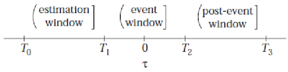
Figure 1: Timeline of an event study
Stock market event studies are premised on the assumption that the stock market operates efficiently and that therefore all information and expectations are included in the current price. All future cash flows that are associated with an event are discounted by the market, based on net present value as soon as the event becomes public. In general, event studies are used to examine the relationship between a firm’s return and the market return over a time prior to the event of interest. If new information becomes available about a firm, the company’s stock might rise or fall depending on the nature of this new information. The prediction error for a firm, the difference between the normal return predicted by the market model for the company and the company’s actual return on a given day, is used as a measure of the abnormal returns attributed to the release of the new information about the company (Hamilton, 1993). The market model assumes that there is a stable linear relation between the market return and the security return. For firm i and event date τ the abnormal return is:
𝐴𝑅𝑖𝜏 = 𝑅𝑖𝜏− 𝐸(𝑅𝑖𝜏|𝑋𝜏)
Where 𝐴𝑅𝑖𝜏, 𝑅𝑖𝜏 and 𝐸(𝑅𝑖𝜏|𝑋𝜏) are the abnormal, actual, and normal returns respectively for
time period τ. 𝑋𝜏 is the conditioning information for the normal return model. This model will
test whether the additional data on ESG provides news to investors, this will be the case if significant abnormal returns are observed. There are several approaches available to calculate a firm’s normal performance, they can be broadly grouped into two categories: statistical models and economic models. For the analysis one of the statistical models is used: the market model. For the use of statistical models, asset returns need to be jointly variate normal and independently and identically distributed through time. However, in practice the violation of
- 18 -
this normality assumption does not lead to problems because it is empirically reasonable and inferences using normal return models tend to be robust from deviations of the assumption (MacKinlay, 1997). For any security 𝑖 the market model is:
𝑅𝑖𝑡 = 𝛼𝑖+ 𝛽𝑖𝑅𝑚𝑡+ 𝜀𝑖𝑡
𝐸(𝜀𝑖𝑡 = 0) 𝑣𝑎𝑟(𝜀𝑖𝑡) = 𝜎𝜀2𝑖
Where 𝑅𝑖𝑡 and 𝑅𝑚𝑡 are the period-t returns on security 𝑖 and the market portfolio, respectively,
and 𝜀𝑖𝑡 is the zero-mean disturbance term. 𝛼𝑖, 𝛽𝑖 and 𝜎𝜀2𝑖 are the parameters of the market model
(MacKinlay, 1997). These parameters are estimated using the ordinary least squares based on an estimation period of [-200,-6] prior to the event, this is consistent with the estimation period used by other researchers, such as 225 days (Small at el., 2007), 150 days (Lummer and McConnel, 1989) and 239 days (Brown and Warner, 1985). Given the market model parameter estimates for each security in the sample, the even-related change or abnormal return can be calculated. Using the market model to measure normal returns, the sample abnormal return is equal to:
𝐴𝑅̂ = 𝑅𝑖𝜏 𝑖𝜏− 𝛼̂ − 𝛽𝑖 ̂ 𝑅𝑖 𝑚𝜏
The abnormal return is the disturbance term of the market model calculated on an out of sample basis. In order to draw overall inferences for the event of interest I must aggregate the abnormal return observations of the individual firms over time. The cumulative abnormal return (CAR) for a single firm is given as:
𝐶𝐴𝑅̂ (𝜏𝑖 1, 𝜏2) = ∑ 𝐴𝑅̂𝑖𝜏 𝜏2
𝜏=𝜏1
Where 𝐶𝐴𝑅̂ (𝜏𝑖 1, 𝜏2) is the cumulative abnormal return for firm 𝑖 over the event period and 𝐴𝑅̂ 𝑖𝜏 is the abnormal return of firm 𝑖 at time 𝑡. Test statistics for significance of the abnormal returns have been derived and tested for a sample of firms in several event studies [Masulis (1980), Holthausen (1981)]. In addition to the parametric statistics, event studies often report nonparametric tests as they do not require stringent assumptions about the return distributions. This paper will use the Wilcoxon signed-rank test as a nonparametric test, which compares the
- 19 -
proportion of negative and positive abnormal returns against an assumed 50 percent split under the null hypothesis of no reaction to the event (Cowan, 1992). There are several reasons to use nonparametric tests over parametric tests. First of all, if there is event related variance increase, standard parametric tests report, more often than expected, a price reaction when actually none exists. As the nonparametric tests do not use return variance they may perform better under variance increases than the parametric tests (Brown and Warner, 1985). Second of all, when the sample includes outliers the result of the parametric test could result from the outlier. Having an outlier leads to a special case of variance increase, and hence the nonparametric tests are also more accurate under these circumstances. Last of all, when the event window increases the use of the parametric test requires an adjustment to reflect autocorrelation in the time series of mean daily abnormal returns, while nonparametric tests do not require this correction.
Because of these reasons and due to the distribution of the asset returns in the dataset used and the fact that they are far from normally distributed, the analysis will be based on the nonparametric Wilcoxon signed-rank test.
5. Empirical results
This part of the paper presents the empirical results for the hypotheses. The results are presented by the usage of tables alongside explanatory statistical tests.
5.1 Descriptive statistics and correlation matrix 5.1.1 Descriptive statistics
Table 2 shows the daily distribution of the return and the corresponding Score-variables as defined in section 4.1. It shows the number of observations, the mean, the standard deviation and the minimum and maximum of the respective variables during the event time. The mean for Score1 and Score2 are relatively similar with 62.39 and 61.56 respectively. Among the events the minimum equals 1.37 for Score1 and 3.41 for Score2. The maximum equals 88.49 for Score1 and 90.34 for Score2. For the event study the change of the Scores 1 and 2 is needed, those are shown in the lower part of the table. The mean daily percentage change is -0.22% for Score1 and -0.19% for Score2, with a minimum of -1.51% and -1.79% respectively. The maximum positive daily change equals for Score1 7.14%, while for Score2 that is 4.39%. The dispersion of the change in the two scores is relatively similar around 1.05%.
- 20 -
Table 2
Overall descriptive statistics
This table presents the overall descriptive statistics for each score during the event day t=0. It shows the number of events for each score and the corresponding mean, standard deviation, minimum and maximum for the equivalent score during a certain event. Data is collected from TruValue Labs.
Score1 Score2 General score Mean 62.39 61.56 Standard deviation 16.80 18.67 Minimum 1.37 3.41 Maximum 88.49 90.34 Percentage change Mean -0.22 -0.19 Standard deviation 1.05 1.04 Minimum -1.51 -1.79 Maximum 7.14 4.39 Nb. of Obs. 725 542
In order to identify a “significant change” in the dataset and hence to identify an event, a daily percentage change of more than three-standard deviations away from the mean daily percentage change of a Score of a single company is considered as an event.
The summary statistics of the events for Score1 are shown on the left-hand side of table 3. In total there are 725 events, with 544 negative events and 181 positive events with an average score of 68.01 and 45.48 respectively. An average percentage change -0.70% for the negative events and an average of 1.28% for the positive events. The smallest positive change considered as a positive event is 0.08%, while the largest one equals 7.14%. Whereas, the largest negative drop that is classified as an event equals -1.51%.
Concerning the summary statistics for Score2 the same approach is used and hence a three-standard deviation change is considered as an event for Score2. The right-hand side of table 3 shows the results of the events based on Score2. In total there are 542 events during the sample time window, with an average score of 68.09 for the negative events and 45.35 for the positive events. The average daily change is equal to -0.74% for the negative events and 1.18% for the positive events. The largest positive change equals 4.39% while the smallest positive change is
- 21 -
equal to 0.2%. For the negative events in Score2 the biggest score drop during the event is equal to -1.79% and the smallest drop is equal to -0.06%.
Table 3
Detailed descriptive statistics
This table presents the detailed descriptive statistics for each type of event during the event day t=0. It shows the number of positive and negative events for each score and the corresponding mean, standard deviation, minimum and maximum for the equivalent score during a certain event. Data is collected from TruValue Labs.
Score1 Score2
Positive events Negative events Positive events Negative events
General score Mean 45.48 68.01 45.35 68.09 Standard deviation 16.74 12.52 17.81 14.60 Minimum 1.37 16.39 3.41 17.88 Maximum 80.79 88.49 79.00 90.34 Percentage change Mean 1.28 -0.72 1.18 -0.74 Standard deviation 1.10 0.31 0.91 0.36 Minimum 0.08 -1.51 0.20 -1.79 Maximum 7.14 -0.16 4.39 -0.06 Nb. of Obs. 181 544 156 386 5.1.2 Correlation Matrix
To determine the variables dependency at the same time, a spearman correlation matrix is performed (table 4). To assess whether there exists a significant relation between two variables in a population based on the sample (a period of 11-days [-5,5] around event date t=0), the following hypothesis is formulated:
Hypothesis 5(0): 𝜌𝑠 = 0 Hypothesis 5(A): 𝜌𝑠 ≠ 0
In which 𝜌𝑠 is defined as the Spearman’s population coefficient. If H5(0) cannot be rejected
- 22 -
Table 4
Spearman correlation matrix
This table presents a Spearman correlation matrix between the daily abnormal return, the daily market return, the Fama and French SMB and HML and the ESG-scores 1 and 2, during the event window [-5,5]. A two-tailed t-test is performed in order to test on the significance of the correlation coefficients. ** and * indicate that Rho is significantly different from zero at the 1% and 5%, respectively.
AR Market Return SMB HML Score1 Score2
AR 1 Market Return -0.0059 1 SMB 0.0567** 0.1898** 1 HML 0.0237** 0.0211* -0.1766** 1 Score1 0.0184* -0.0021 -0.0072 0.0063 1 Score2 0.0173* 0.0004 -0.0154 0.0069 0.7414** 1
The Spearman correlation matrix gives a first indication about the direction and significance between different variables. There appears to be a significant positive relation between the Fama and French size and value factor and the abnormal return, which is in accordance with their research (Fama and French, 1996). Additionally, both ESG-scores appear to have a significant positive correlation with abnormal return, indicating that a higher environmental overall score explains (part of) the abnormal return during the considered event window [-5,5]. Based on the nature of Score1 and Score2 it is not surprising that we find a significant positive correlation of 0.7414 between Score1 and Score2
5.2 Inferential statistics 5.2.1 Testing for normality
When data is normally distributed it allows the use of parametric tests to determine statistical significance. However, more often than not this assumption is violated and hence testing for normality is of the essence. Testing for normality is done by looking at the distribution of (cumulative) average abnormal returns over the complete sample and subsamples. The tests are performed for the event date and the two event windows. Table 5 shows the results of a commonly used statistical test with a null hypothesis of normal distribution: the Shapiro-Wilk W test for normal data. Another commonly used practice is to look at the skewness and kurtosis of the data.
The Shapiro-Wilk W test is a strong test (Royston, 1995) of departure from normality, first proposed by Shapiro and Wilk in 1965. The W can be interpreted as a measure of the straightness of the line in a probability plot, low p-values indicate a deviation of normality. The
- 23 -
skewness and kurtosis are used to see whether there occurs deviation from the values of a normal distribution (zero for the skewness and 3 for the kurtosis).
The results in table 5 show, that for the complete sample and for the individual subsamples, there is significant deviation from a normal distribution. The Shapiro-Wilk test is significant at the 1% level for every (sub)sample. These results do not necessarily mean that all parametric tests are considered invalid, but it shows that next to the parametric tests, nonparametric tests are needed to confirm the results.
Table 5
Normal distribution test of full sample
This table presents normal distribution tests for the different events and event windows of interest. *, **, and *** indicate significance at the 10%, 5%, and 1% level.
Shapiro-Wilk (W) Skewness Kurtosis Full sample t=0 0.768*** -4.929 94.163 [-1,1] 0.710*** 2.706 68.925 [-1,3] 0.831*** 1.321 27.934
Positive event score1 t=0 0.478*** -7.927 89.792
[-1,1] 0.715*** -4.095 39.030
[-1,3] 0.822*** -2.241 21.611
Negative event score1 t=0 0.952*** -0.183 6.327
[-1,1] 0.901*** 1.232 10.487
[-1,3] 0.914*** 1.080 11.963
Positive event score2 t=0 0.917*** 0.920 7.663
[-1,1] 0.655*** 3.819 40.571
[-1,3] 0.743*** 3.287 30.611
Negative event score2 t=0 0.940*** -0.326 6.652
[-1,1] 0.602*** 6.649 100.252
[-1,3] 0.794*** 2.915 36.787
5.2.2 Statistical results
In order to test for hypothesis 1 and 2 the statistical significance of the abnormal returns is assessed by separating the positive and negative events of Score1 and Score2. Table 6 shows
the results for the average abnormal return of the event date (AAR0) and the cumulative average
abnormal returns (CAAR) of the periods [-1,1] and [-1,3]. The corresponding z-statistics (for the nonparametric test) and t-statistics (for the parametric test) of the variables are given in
- 24 -
column 2. Column 3 shows the portion of positive (cumulative) average abnormal returns against negative (cumulative) average abnormal returns.
Table 6
Average abnormal return and cumulative average abnormal return
This table presents the average daily change in the firm’s market value around the date of a three standard deviation change in ESG-score estimated on a 195 day interval [-200,-6]. AAR[t=0] indicates the average abnormal return on the day of the event. CAAR[-1,1] gives the cumulative average
abnormal return over a 3-day window. CAAR[-1,3] gives the cumulative average abnormal return over a 5-day window. Abnormal returns (AR) are
given in percentages. Data is collected from TruValue Labs. T-values (Z-values) for mean (median) stock price reactions are from a one-sample t-tests (Wilcoxon signed-rank test). *, **, and *** indicate that the mean (median) daily percentage change is significantly different at the 10%, 5%, and 1% level. Note: the Wilcoxon signed-rank test tests whether the median is different from 0, while AR(%) is the mean abnormal return and hence there can occur a difference in sign.
Score1 Score2
Positive events Negative events Positive events Negative events
AR(%) (z-value) t-value Positive/ Negative AR(%) (z-value) t-value Positive/ Negative AR(%) (z-value) t-value Positive/ Negative AR(%) (z-value) t-value Positive/ Negative AAR [t=0] -0.237 (-.995) -1.240 83/ 98 -0.089 (-1.822)* -1.669* 255/ 289 0.097 (0.364) 0.801 79/ 77 -0.127 (-2.040)** -1.769* 171/ 215 CAAR [-1,1] -0.190 (-0.342) -0.699 87/ 94 0.085 (-0.512) 0.881 264/ 280 0.150 (-0.239) 0.502 74/ 82 -0.135 (-1.900)* -0.803 179/ 207 CAAR [-1,3] -0.118 (-0.375) -0.367 83/ 98 -0.013 (-0.935) -0.095 255/ 289 0.044 (-0.917) 0.128 68/ 88 -0.190 (-1.951)* -1.040 174/ 212 Nb. of Obs. 181 544 156 386
To test hypothesis 1 and 2 the positive and negative events are separated by Score. For each subsample the null hypothesis is that the (cumulative) average abnormal return equals zero across the event period, if a significant deviation appears, the change in ESG-score had a discernible effect on the firm’s stock price. For Score1 the average abnormal return on the event date (t=0) is negative for both events, -0.237% for positive events and -0.089% for negative events. However, only the negative event appears to be statistically significant at the 10%-level. The cumulative average abnormal return in a 3-day (5-day) event window is -0.190% (-0.188%) for the positive event and 0.085% (-0.013%) during the negative event. This shows that the CAAR after a 3-day window is negative (positive) for a positive (negative) event. While for the 5-day window both events have a negative cumulative abnormal return, however, not statistically significant.
Events based on Score2 show slightly different results compared to events based on Score1. The average abnormal return on the event date (t=0) is a positive 0.097% for positive events
- 25 -
and a negative 0.127% during negative events. In which the negative event is statistically significant at the 10%-level when the parametric test is considered and at the 5%-level when the nonparametric test is considered. The cumulative average abnormal return in a 3-day (5-day) event window is 0.150% (0.044%) for the positive event and -0.135% (-0.190%) during the negative event. This shows, in contrast to Score1 events, that the CAAR after a 3-day and 5-day window is positive (negative) for a positive (negative) event. However, only the negative Score2 events appear to be statistically significant at the 10%-level when the nonparametric test is considered.
The results show that on the one hand the magnitude of the impact is low for positive ESG Score1 events. So, H1(0) cannot be rejected, since the average change in a firm’s market value around a positive event date is barely significant. On the other hand, negative events appear to have a statistically significant negative reaction on the firm value after a negative change in the score. For Score1, this only appears during the event date itself (t=0) at the 10%-significance level. While, for Score2, this appears at the event date (t=0) at the 5%-significance level and for the 3-day and 5-day event window at the 10%-significance level. These results give strong support to H2(A) during the event date (t=0) and moderate support during the 3-day and 5-day event window.
Table 7
Average abnormal return and cumulative average abnormal return (high and low ESG-score)
This table presents the average daily change in the firm’s market value around the date of a three standard deviation change in ESG-score estimated on a 195 day interval [-200,-6]. AAR[t=0] indicates the average abnormal return on the day of the event. CAAR[-1,1] gives the cumulative average abnormal return over a 3-day
window. CAAR[-1,3] gives the cumulative average abnormal return over a 5-day window. Abnormal returns (AR) are given in percentages. Data is collected from
TruValue Labs. Returns in bold show the higher return on a given event (in absolute terms). T-values (Z-values) for mean (median) stock price reactions are from a one-sample t-tests (Wilcoxon signed-rank test), or for the difference from a two-sample t-test (Mann-Whitney test). *, **, and *** indicate that the mean (median) daily percentage change is significantly different at the 10%, 5%, and 1% level. Note: the Wilcoxon signed-rank test tests whether the median is different from 0, while AR(%) is the mean abnormal return and hence there can occur a difference in sign.
Score1 Score2
Positive events Negative events Positive events Negative events
ESG- score AR(%) (z-value) p-value Positive/ Negative AR(%) (z-value) p-value Positive/ Negative AR(%) (z-value) p-value Positive/ Negative AR(%) (z-value) p-value Positive/ Negative AAR [t=0] Above average -0.385 (-0.849) -1.159 44/ 49 -0.124 (-2.275)** -1.789* 130/ 168 0.144 (1.309) 1.044 47/ 33 -0.092 (-1.569) -1.152 105/ 129 Below average -0.080 (-0.528) -0.452 39/ 49 -0.047 (-0.131) -0.563 125/ 121 0.047 (-0.828) 0.232 32/ 44 -0.180 (-1.340) -1.341 67/ 86 Difference 0.305 (0.136) 0.811 88/ 93 0.077 (1.521) 0.716 298/ 246 -0.098 (-1.408) -0.399 76/ 80 -0.088 (-0.165) -0.564 153/ 234
- 26 - CAAR [-1,1] Above average -0.290 (-0.167) -0.666 43/ 50 0.071 (-0.674) 0.583 136/ 159 0.344 (0.691) 1.338 41/ 39 0.024 (-0.856) 0.101 114/ 120 Below average -0.085 (-0.312) -0.265 44/ 44 0.101 (-0.044) 0.659 128/ 121 -0.054 (-1.035) -0.098 33/ 43 -0.381 (-1.834)* -1.632 65/ 87 Difference 0.205 (-0.148) 0.379 88/ 93 0.030 (0.341) 0.153 249/ 295 -0.399 (-1.237) -0.655 76/ 80 -0.404 (-1.108) -1.225 152/ 234 CAAR [-1,3] Above average -0.263 (0.012) -0.554 46/ 52 -0.013 (-0.795) -0.080 131/ 160 0.427 (0.552) 1.285 40/ 42 -0.109 (-1.336) -0.445 105/ 124 Below average 0.054 (-0.595) 0.127 37/ 46 -0.012 (-0.554) -0.057 124/ 129 -0.379 (-1.818)* -0.601 28/ 46 -0.308 (-1.436) -1.125 69/ 88 Difference 0.316 (-0.473) 0.499 83/ 98 0.000 (0.068) 0.001 253/ 291 -0.806 (-1.821) -1.130 74/ 82 -0.200 (-0.354) -0.545 157/ 229
Testing hypothesis 3 is conducted in the same manner as described above (comparing the (cumulative) average abnormal return with zero). The nonparametric two-sample t-tests (Mann-Whitney test) is used to test whether companies with a higher ESG-score react less to events compared to companies with a lower ESG-score. The results are presented in table 7. There are two cases in which the below average ESG-score companies earn a significantly negative cumulative abnormal return (at the 10%-level), while the above average ESG-score companies do not earn a significant abnormal return. For the 5-day (3-day) event window the cumulative abnormal return of a positive (negative) event in Score2 is equal to -0.379% (-0.381%), however, the difference between the above and below average scores does not appear to be significantly different with a z-value of -1.821 (-1.108). There is one case in which the above average ESG-score companies earn a significantly negative abnormal return (at the 5%-level), while the below average ESG-score companies do not earn a significantly abnormal return. For the Score1 negative event date, the above average group earns a significantly negative abnormal return of -0.124%. However, the difference between the below and above average group does not appear to be significantly different (z-value equal to 1.521).
Although the differences do not appear to be statistically significant, and hence we cannot reject
H3(0), there is a pattern in absolute terms. For all the events based on Score2, companies with
an above average ESG-score have a higher (cumulative) average abnormal return compared to companies with a below average ESG-score. To the contrary, if events are based on Score1, the companies with a below average ESG-score appear to generate a higher abnormal return (in absolute terms) then the companies with an above average ESG-score.
- 27 -
This part of the paper performs several robustness checks with regards to the event study. It alters some of the assumptions underlying the model.
6.1 Alteration of event criteria
For the base case scenario, a three-standard deviation increase is considered as an event, for this robustness check the threshold is lowered to a two-standard deviation change to see whether the results are robust. Table 8 shows the results for the average abnormal return of the event
date (AAR0) and the cumulative average abnormal returns (CAAR) of the periods 1,1] and
[-1,3]. The corresponding z-statistics and t-statistics of the variables are given in column 2. Column 3 shows the portion of positive (cumulative) average abnormal returns against negative (cumulative) average abnormal returns. Interesting is that even though the threshold is decreased from three standard deviations to two standard deviations the number of events analyzed is less than for the three-standard deviation threshold. This is due to clustering concerns, which requires the removal of events that are overlapping in the estimation period. Therefore, the number of events available for the event study is less, even though in total more events occurred.
Table 8
Average abnormal return and cumulative average abnormal return (lower standard deviation)
This table presents the average daily change in the firm’s market value around the date of a two standard deviation change in ESG-score estimated on a 195 day interval [-200,-6]. AAR[t=0] indicates the average abnormal return on the day of the event. CAAR[-1,1] gives the cumulative average
abnormal return over a 3-day window. CAAR[-1,3] gives the cumulative average abnormal return over a 5-day window. Abnormal returns (AR) are
given in percentages. Data is collected from TruValue Labs. T-values (Z-values) for mean (median) stock price reactions are from a one-sample t-tests (Wilcoxon signed-rank test). *, **, and *** indicate that the mean (median) daily percentage change is significantly different at the 10%, 5%, and 1% level. Note: the Wilcoxon signed-rank test tests whether the median is different from 0, while AR(%) is the mean abnormal return and hence there can occur a difference in sign.
Score1 Score2
Positive events Negative events Positive events Negative events
AR(%) (z-value) t-value Positive/ Negative AR(%) (z-value) t-value Positive/ Negative AR(%) (z-value) t-value Positive/ Negative AR(%) (z-value) t-value Positive/ Negative AAR [t=0] -0.470 (-0.092) -0.709 25/ 23 -0.141 (-1.904)* -1.732* 113/ 151 0.022 (0.099) 0.211 41/ 44 -0.143 (-1.798)* -1.778* 118/ 158 CAAR [-1,1] -0.822 (-0.072) -0.967 24/ 24 0.028 (-0.439) 0.208 119/ 145 0.029 (1.172) 0.137 49/ 36 -0.219 (-1.431) -1.421 122/ 154 CAAR [-1,3] -0.858 (-0.062) -0.866 24/ 24 0.145 (-0.400) 0.742 118/ 146 -0.135 (-0.716) -0.394 36/ 49 -0.261 (-1.744)* -1.393 127/ 149 Nb. of Obs. 48 264 85 276