Water vapour profiles by ground-based FTIR spectroscopy: study for an optimised retrieval and its validation

(1)

www.atmos-chem-phys.net/6/811/2006/ © Author(s) 2006. This work is licensed under a Creative Commons License.

Chemistry

and Physics

Water vapour profiles by ground-based FTIR spectroscopy:

study for an optimised retrieval and its validation

M. Schneider, F. Hase, and T. Blumenstock

IMK-ASF, Forschungszentrum Karlsruhe and Universit¨at Karlsruhe, Germany

Received: 7 July 2005 – Published in Atmos. Chem. Phys. Discuss.: 29 September 2005 Revised: 19 January 2006 – Accepted: 25 January 2006 – Published: 14 March 2006

Abstract.The sensitivity of ground-based instruments

mea-suring in the infrared with respect to tropospheric water vapour content is generally limited to the lower and mid-dle troposphere. The large vertical gradients and variabili-ties avoid a better sensitivity for the upper troposphere/lower stratosphere (UT/LS) region. In this work an optimised re-trieval is presented and it is demonstrated that compared to a commonly applied method, it improves the performance of the FTIR technique. The reasons for this improvement and the possible deficiencies of the method are discussed. Only by applying the method proposed here and using measure-ments performed at mountain observatories can water vapour variabilities in the UT/LS be detected in a self-consistent manner. The precision, expressed as noise to signal ratio, is estimated at 45%. In the middle and lower troposphere, precisions of 22% are achieved. These estimations are con-firmed by a comparison of retrieval results based on real FTIR measurements with coinciding measurements of syn-optical meteorological radiosondes.

1 Introduction

The composition of the Earth’s atmosphere has been pro-foundly modified throughout the last decades mainly by hu-man activities. Prominent examples are the stratospheric ozone depletion and the upward trend in the concentration of greenhouse gases. While studies about the stratospheric composition have progressed rather well, there still exists a considerable deficiency for data from the free troposphere. Knowing the composition and evolution of these altitude re-gions is essential for the scientific verification of the Kyoto and Montreal Protocols and Amendments and for global cli-mate modelling. Water vapour is the dominant greenhouse

Correspondence to:M. Schneider (matthias.schneider@imk.fzk.de)

gas in the atmosphere, and in particular its concentration and evolution in the upper troposphere and lower stratosphere (UT/LS) are of great scientific interest for climate modelling (Harries, 1997; Spencer and Braswell, 1997). Currently there is no outstanding routine technique for measuring wa-ter vapour in the UT/LS. The quick changes of atmospheric water vapour concentrations with time, their large horizontal gradients, and their decrease of several orders of magnitude with height makes their accurate detection a challenging task for any measurement technique. Traditionally tropospheric water vapour profiles are measured by synoptical meteoro-logical radiosondes. However, this method has some defi-ciencies at altitudes above 6–8 km, which are mainly due to uncertainties in the pre-flight calibration and temperature de-pendence (Miloshevich, 2001; Leiterer et al., 2004). Other applied techniques are remote sensing from the ground by Lidar or Microwave instruments. Both are limited in their sensitivity: the Lidar generally to below 8–10 km, and the microwave measurements to above 15 km (SPARC, 2000). Satellite instruments also struggle to reach below this alti-tude. In this context the suggested formalism of retrieving upper tropospheric water vapour amounts from ground-based FTIR measurements aims to support efforts to obtain qual-ity UT/LS water vapour data for research. To our knowl-edge, it is the first time that water vapour profiles measured by this technique are presented. A great advantage is that high quality ground-based FTIR measurements have already been performed during the last 10–15 years within the Net-work for Detection of Stratospheric Change (Kurylo, 1991, 2000; NDSC, web site). Therefore a long-term record of wa-ter vapour could be made available, with both temporal and to some extent, spatial coverage.

(2)

5 10 15

100 101

102 103

104

5 10 15

altitude [km]

al

ti

tude [km

]

-0.64 -0.52 -0.40 0.40 0.52 0.64 0.76 0.88 1.00

volume mixing ratios [ppmV]

al

tit

ude [

k

m

]

mean standard deviation

Fig. 1.Description of a-priori state. Left panel: correlation matrix.

Right panel: black line: mean state; red line: standard deviation of mean state.

quantitative estimations about the expected improvements to these qualitative considerations. It is also shown how possi-ble deficiencies of the optimised method can be eliminated. Finally, these estimations are validated by a comparison of retrieval results based on real measurements with coinciding in-situ measurements.

2 Optimised water vapour retrieval

An inversion problem is generally under-determined. Many state vectors (x) are consistent with the measurement vector (y). If one also considers measurement noise (ǫy), there is an even wider range of possible solutions withinǫy, in ac-cordance to the measurement vector: in the equation,

ˆ

y₌y₊ǫy =Kx (1)

the matrixKis ill-conditioned. Its effective rank is smaller than the dimension of state space, i.e. it is singular and cannot be simply inverted. To come to an unique solution ofx, the state space is constrained by requiring:

Bx₌Bxa (2)

where xa is a “typical” or a-priori state and the matrix B determines the kind of required similarity ofxwithxa. This equation constrains the solution independently from the mea-surement, i.e. before the measurement is made. ThereforeB

andxacontain the kind of information known about the state prior to the measurement. Subsequently, assuming Gaussian statistics for the error term in Eq. (1) and the a-priori distri-bution in Eq. (2) leads to the cost function:

σ−2(y₋Kx)T(y₋Kx)₊(x₋xa)TBTB(x−xa) (3) The most probable state is the one which minimises Eq. (3). Here (ǫ_yTǫy)−1 was identified by σ−2. It is obvious that the applied a-priori information (B and xa) influences the solution. For water vapour the large amount of synopti-cal meteorologisynopti-cal sonde (ptu-sonde) data allows a detailed

study of the a-priori state. In the following it is discussed whether the extensive a-priori information can be used to op-timise the performance of the retrieval. The study of a-priori data is done for the island of Tenerife, where ptu-sondes are launched twice daily (at 00:00 and 12:00 UT) within the global radiosonde network and where an FTIR instrument has been operating since 1999 at a mountain observatory (Iza˜na Observatory, Schneider et al., 2005).

2.1 Characterisation of a-priori data

The study is based on the daily 12:00 UT soundings per-formed from 1999 to 2003. It has been observed that an in-situ instrument – located at the mountain observatory – and the sonde, when measuring at the observatory’s alti-tude, detect quite different humidities because of their dif-ferent locations, i.e. on the surface and in the free tropo-sphere (see Sect. 4). For this reason the analysed profiles are built up by a combination of the in-situ measurements at the instrument’s site (for the lowest grid point; applied sensor: Rotronic MP100H), and sonde measurements (for all other grid points below 16 km). For higher altitudes a mean mix-ing ratio of 2.5 ppmv and covariances like those at 16 km are applied. The left panel of Fig. 1 shows the correlation matrix

Ŵadetermined from these a-priori profiles. Here correlation

matrices are presented instead of the commonly shown co-variance matrixes. The reason is that they can be more eas-ily presented. Their elements are all of the same order of magnitude (between₋1 and 1), whereas in the case of water vapor the elements of the covariance matrices extend over 8 orders of magnitude. Figure 1 demonstrates how variabili-ties at different altitudes typically correlate with each other. In the real atmosphere the mixing ratios for different alti-tudes show correlation coefficients of at least 0.5 within a layer of around 2.5 km. The a-priori covariance matrixSa

is calculated fromŴaby Sa=6aŴa6aT, where6a is a

di-agonal matrix containing the a-priori variabilities at a certain altitude. These variabilities are depicted as a red line in the right panel of Fig. 1. The black line shows the mean mixing ratios. The determined mean and covariances only describe the whole ensemble completely if mixing ratios are normally distributed. This is generally assumed and often justified by the fact that entropy is then maximised: if only the mean and the covariance are known a supposed normal distribution is thus the least restricting assumption about the a-priori state (Sect. 10.3.3.2 in Rodgers, 2000). However, this does not necessarily reflect the real situation!

A further examination of the sonde data reveals that the mixing ratios at a certain altitude are not normally but log-normally distributed. Their pdf is:

Px =

1

xσ√2πexp−

(lnx₋lnxa)2

2σ2 (4)

(3)

xabetween 5000 ppmv close to the surface and 1.5 ppmv in the stratosphere. The only exception of this distribution is the first_≈100 m above the surface, where the mixing ratios are more normally distributed. It is possible to sample all this additional information in a simple mean state vector and a covariance matrix. This is achieved by transforming the state on a logarithmic scale, which transforms the log-normal pdf to a normal pdf. A normal pdf can be completely described by its covariance and its mean. Aχ2-test reveals how the description of the a-priori state is improved by this transfor-mation. This test determines the probability of a particular random vector of belonging to an assumed normal distribu-tion. If a vectorxis supposed to be a member of a Gaussian ensemble with the meanxa and covariance S the quantity considered is:

χ2₌(x₋xa)TS−1(x−xa) (5)

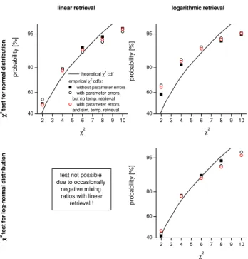
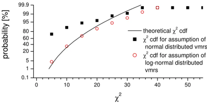
Theχ2test clearly rejects a normal distribution of the mixing ratios. This can be seen by comparing the theoretical cumula-tive distribution function (cdf) ofχ2with the one determined by Eq. (5). Figure 2 demonstrates that the theoreticalχ2

cdf differs clearly from the cdf obtained from the ensemble’s state vectors if they are assumed to be normally distributed (difference between black line and black squares). More than 95% of the ensemble’s state vectors are not consistent with this assumption. On the other hand, a prior log-normal pdf is well confirmed. If the mixing ratios and the covariances are transformed to a logarithmic scale, only approximately 10% of the ensemble’s states fail the test (compare black line and red circles).

2.2 Discussion of two retrieval methods

This section discusses the differences between an inversion performed on a linear scale, which is the method commonly used for trace gas retrievals, and one performed on a logarith-mic scale. The logarithlogarith-mic retrieval is occasionally applied as a positivity constraint, since it avoids negative components in the solution vector. In the case of water vapour it has a further advantage. It converts the state for which Eq. (3) minimises in a statistically optimal solution: on a logarith-mic scale the a-priori state can be described correctly in the form of a mean and covariance. Under these circumstances, substitutingBTBandxain Eq. (3) by the inverse of the loga-rithmic a-priori covariance (Sa−1) and the median state vec-tor, leads to a cost function, which is directly proportional to the negative logarithm of the a-posteriori probability density function (pdf) of the Bayesian approach. This posterior pdf is the conditional pdf of the state given the measurement, or in other words, the a-priori pdf of the state updated by the information given in the measurement. The minimisation of Eq. (3) thus yields the maximum a-posteriori solution, i.e. it is the most probable state given the measurement.

To the contrary, on a linear scale settingBTBasSa−1and

xa as mean state in Eq. (3) does not lead to a statistically

0 10 20 30 40 50

0.1 1 5 20 40 60 80 95 99 99.9

theoretical χ2

cdf χ2

cdf for assumption of normal distributed vmrs

χ2

cdf for assumption of log-normal distributed vmrs

probabilit

y [

%

]

χ2

Fig. 2. χ2test for different of a-priori assumptions. Black line:

theoreticalχ2 cumulative distribution function (cdf); black filled squares: χ2cdf of ensemble for assumed normal pdf on a linear scale; red circles:χ2cdf of ensemble for assumed normal pdf on a logarithmic scale.

optimal solution. It is not related to the a-posteriori pdf in the Bayesian sense. On a linear scale the a-priori state is log-normally distributed. Therefore, seen from a statistical point of view, the second term of the cost function over-constrains states above the mean and under-constrains states below the median. As a consequence, the probability of states above the mean is underestimated and below the median overestimated – the overestimation is greater the further away it is from the centre of the a-priori distribution. Thus, if compared to a correct maximum a-posteriori solution, the retrieval tends to underestimate the values of the real state both far above and far below the mean state.

However, the transformation on a logarithmic scale in-troduces some other problems: it significantly increases the non-linearity of the forward model, which requires decreas-ing the differences between each iteration step, thus lower-ing the speed of convergence. This difficulty is overcome within the inversion code PROFFIT by using a refined min-imisation scheme. A further drawback is that, in the retrans-formed linear scale the constraints now depend on the solu-tion, which may cause misinterpretations of the spectra. To assess whether the linear or logarithmic retrieval performs better both retrieval approaches are extensively examined first by a theoretical (Sect. 3) and second by an empirical validation (Sect. 4).

2.3 Applied inversion code and spectral region

(4)

1110 1111 1112 0

1 2 3 4

1117.5 1121 1122 H₂O

measurement retrieval residuum

x 10

abs

olute r

adianc

es

[W

/(

c

m

2s

ter

ad c

m

-1)]

H₂O

x 10

wavenumber [cm-1

]

H₂O H₂O

x 10

Fig. 3.Spectral regions applied for retrieval. Plotted is the situation

for a real measurement taken on 10 March of 2003 (solar elevation angle 50◦). Black line: measured spectrum; red line: simulated spectrum; green line: difference between simulation and measure-ment.

a-priori value for the measurement noise (σ of Eq. 3). This value is taken from the residuals of the fit itself, performing an automatic quality control of the measured spectra. Fur-thermore, if the observed absorptions depend on tempera-ture, PROFFIT allows the retrieval of temperature profiles. For both the linear and logarithmic retrieval, the same re-trieval setup is applied: three microwindows between 1110 and 1122 cm−1 are fitted. Figure 3 shows a typical situa-tion for an evaluasitua-tion of a real measurement. The black line represents the measurement, the red dotted line the simulated spectrum and the green line the difference between both. The H2O signatures are marked in the Figure. One can observe

that two stronger lines (at 1111.5 and 1121.2 cm−1) and two relatively weak lines (at 1117.6 and 1120.8 cm−1) lie within these spectral regions, where additionally O3is an important

absorber (numerous thin strong signatures). The profile of this species is thus simultaneously retrieved. Other interfer-ing gases are CO2, N2O, and CH4, whereby the latter two

are also simultaneously retrieved by scaling their respective climatological profiles, the former is kept fixed to a climato-logical profile. Spectroscopic line parameters are taken from the HITRAN 2000 database Rothman et al. (2003), except for O3, where parameters from Wagner et al. (2002) are

ap-plied.

3 Error analysis and sensitivity assessment

Assuming linearity for the forward modelF and the inverse modelIwithin the uncertainties of the retrieved state and the model parameters it is (Rodgers, 2000):

ˆ

x₋x₌∂I[F(xˆ,pˆ),pˆ]

∂y

∂F(x_ˆ,p_ˆ)

∂x −I

(x₋xa)

+ ∂I[F(_∂xˆ_y,pˆ),pˆ]∂F_∂(x_pˆ,pˆ)(p₋pˆ)

+ ∂I[F(_∂xˆ_y,pˆ),pˆ](y₋yˆ)

=(Aˆ ₋I)(x₋xa)+ ˆGKpˆ (p−pˆ)+ ˆG(y−yˆ) (6) i.e. the difference between the retrieved and the real state (xˆ₋x) – the error – can be linearised about a mean profile xa, the estimated model parameters p, and the measuredˆ spectrumy. Hereˆ Iis the identity matrix, Aˆ the averaging kernel matrix,Gˆ the gain matrix, andKpˆ a sensitivity matrix to model parameters:

ˆ A_{= ˆ}GKˆ

ˆ

G₌∂I[F(xˆ,pˆ,pˆ]

∂y

ˆ

K₌∂F(xˆ,pˆ)

∂x

ˆ

Kp=

∂F(x_ˆ,p_ˆ)

∂p (7)

wherebyKˆ is the Jacobian. Equation (6) identifies three prin-ciple error sources. These are the inherent finite vertical res-olution, the input parameters applied in the inversion proce-dure, and the measurement noise. This analytic error estima-tion may be applied if the inversion is performed on a linear scale. In this case, the constraints and consequentlyGˆ are constant within the uncertainty ofx. However, if the inver-ˆ sion is performed on a logarithmic scale the constraints are constant on this scale, but variable on the retransformed lin-ear scale. Changes of the state vector towards values above the a-priori value are only weakly constrained, while changes towards smaller values are more strongly constrained. As a consequenceGˆ cannot necessarily be considered constant within the uncertainty of the retrieved state and some model parameters. The latter is particularly problematic for water vapour. The phase error of the instrumental line shape and the temperature profile have a large impact on the spectra. This is due to the broad and strong absorption signatures of water vapor. Consequently, all these errors can only be es-timated by a full treatment. Two forward calculations are performed for each error estimation and for all profiles of the large ensemble of the a-priori profiles: a first calculation with correct parameters and a second with erroneous parameters. Subsequently both spectra are retrieved with the correct pa-rameter as input data. The papa-rameter error is then given by the difference of the two retrievals. The smoothing error is the difference between the correct parameter retrieval and the a-priori profile. In this work, all errors are estimated by this full treatment for consistency reasons for both the linear and the logarithmic retrieval.

(5)

ˆ

A) are used to estimate the sensitivity of the retrieval at cer-tain altitudes. They document by how much ppmv the re-trieved solution will change due to a variability of 1 ppmv in the real atmosphere. They may inform that 1 ppmv more at 5 km is reflected in the retrieval by an extra of 0.1 ppmv at 8 km. However, the typical real atmospheric variabilities at different altitudes are not considered and hence to what ex-tent the typical variability as retrieved at 8 km is disturbed by typical variabilities at 5 km. This is a minor problem if the mixing ratio variabilities have the same magnitude through-out the atmosphere. The variabilities of water vapour de-crease by 3–4 orders of magnitude from the surface to the tropopause (see Fig. 1), thus the interpretation of the averag-ing kernels is quite limited. Alternatively, one may produce adequately normed kernels to address this deficiency. Fur-thermore the averaging kernels depend strongly on the ac-tual water vapor content, i.e. there is no typical kernel and non-linearities play an important role. For all these reasons here a full treatment, consisting of forward calculation of as-sumed real states and subsequent inversion, is used to esti-mate the response of the retrieval on real atmospheric vari-abilities. Therefore, the real state vectors are correlated lin-early to their corresponding retrieved vectors. The correla-tion coefficient (ρ) considers the different magnitudes of the variabilities. For instance,ρ between the real state at 5 km and the retrieved state at 8 km gives the typical fraction of the retrieved variabilities at 8 km due to disturbances from 5 km. These correlation matrices give a good overview of the rela-tion between real atmospheric variabilities and the retrieved variabilities.

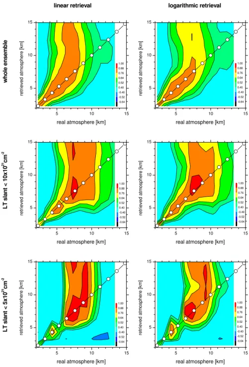
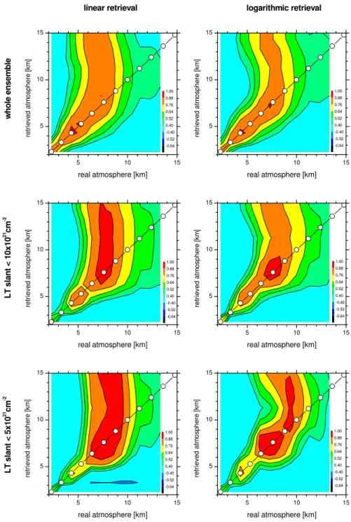
Error estimation and sensitivity assessment are performed for the whole ensemble (the ensemble used for calculat-ing the a-priori mean and covariances), and for two sub-ensemble of selected conditions, when especially good upper tropospheric sensitivity and even sensitivity in the tropopause region are expected. Sensitivity in the UT and tropopause re-gion requires the strong absorption lines to be unsaturated. Furthermore, the signal to noise ratio, which at Iza˜na is oc-casionally decreased by high aerosol loading owing to Sa-haran dust intrusion events, should be acceptable (above 200 at 1100 cm−1). In 30% of all measurement days the lower tropospheric water vapour slant column amounts (slant column amounts between surface and 4.3 km) are below 10×1021 cm−2(LT slant<10×1021cm−2criterion), which means that the strong absorption lines are unsaturated. On these days, good sensitivity for the UT can be expected. The observing system should perform even better if the lower tro-pospheric slant column amounts are below 5_×1021cm−2(LT slant <5_×1021 cm−2 criterion). This is however only the case for 10% of all possible observations.

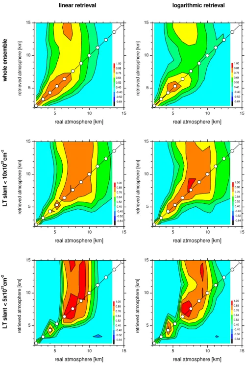
3.1 Smoothing error

Figure 4 shows correlation matrices in the absence of param-eter errors. They document the sensitivity of the retrieval

if the smoothing error alone is taken into account. The left panels show the linear retrieval, the right panels the loga-rithmic retrieval, the upper panels the whole ensemble, and the middle and lower panels the LT slant<10×1021 cm−2 and LT slant<5×1021 cm−2 sub-ensembles. Considering the whole ensemble the sensitivity is limited to altitudes be-low 8–9 km. Furthermore, the upper tropospheric mixing ratios of the linear retrieval tend to depend more on variabil-ities at lower altitudes. For example, the value retrieved at 9 km is mainly influenced by the real atmospheric situation at 7 km. This incorrect altitude attribution is less pronounced in the logarithmic retrieval. For the LT slant<10×1021cm−2 sub-ensemble the sensitivity is extended by 1–2 km towards higher altitudes. In this case, the observing system provides good information about the atmospheric water vapour vari-abilities up to 10 km (ρat the diagonal above 0.7). As before, for the linear retrieval, the amounts at higher altitudes are strongly disturbed by the real states at lower altitudes, while, for the logarithmic retrieval, high correlation coefficients are more concentrated around the diagonal of the matrix. If the LT slant is smaller than 5×1021 cm−2, the logarithmic re-trieval’sρvalues at the diagonal are still 0.7 at 11 km. The

ρ values of the linear retrieval are slightly lower (0.61 at 11 km). But the most pronounced difference between both methods is the incorrect altitude attribution in case of the lin-ear retrieval. For example, the mixing ratio retrieved by the linear method at 11 km is strongly correlated to real values at 8 km (ρof 0.9). These disturbances are significantly reduced in case of the logarithmic retrieval (ρof 0.63). Thus the error of the state retrieved with the logarithmic method at 11 km can already be sufficiently reduced by considering the distur-bances originating from altitudes down to about 8 km only. The linear method, on the other hand, should very likely take into account values from further down in order to reach a similar error level. This means that the correlation length of the smoothing error is larger for the linear retrieval. To de-termine the amount of a layer with a certain uncertainty the layer must be broader for the linear retrieval if compared to the logarithmic retrieval.

(6)

5 10 15 5

10 15

real atmosphere [km]

re

tr

ie

ved atm

o

spher

e [km

]

-0.64 -0.52 -0.40 0.40 0.52 0.64 0.76 0.88 1.00

5 10 15

L

T

slan

t <

5x10

21 cm -2 L

T

slan

t <

10x10

21 cm -2 w

h

o

le en

sem

b

le

linear retrieval logarithmic retrieval

re

tr

ie

ved atm

o

spher

e [km

]

-0.64 -0.52 -0.40 0.40 0.52 0.64 0.76 0.88 1.00

5 10 15

re

tr

ie

ved atm

o

spher

e [km

]

-0.64 -0.52 -0.40 0.40 0.52 0.64 0.76 0.88 1.00

5 10 15

re

tr

ie

ved atm

o

spher

e [km

]

-0.64 -0.52 -0.40 0.40 0.52 0.64 0.76 0.88 1.00

5 10 15

re

tr

ie

ved atm

o

spher

e [km

]

-0.64 -0.52 -0.40 0.40 0.52 0.64 0.76 0.88 1.00

5 10 15

re

tr

ie

ved atm

o

spher

e [km

]

-0.64 -0.52 -0.40 0.40 0.52 0.64 0.76 0.88 1.00

Fig. 4.Sensitivity of observing system in the absence of parameter error. Depicted are correlation matrices between assumed real profiles

and retrieved profiles. Left panels for retrieval on a linear scale, right panels for retrieval on a logarithmic scale. Upper panels for the whole ensemble, middle panels for the LT slant<10×1021cm−2sub-ensemble, and lower panels for the LT slant<5×1021cm−2sub-ensemble. Colors mark the values of the correlation coefficients (ρ) as given in legend.

the real atmosphere – as a mean – is mapped by the retrieval: their difference from the diagonal describes the systematic smoothing error. The scattering around the regression curve describes its pure random error. For a linear least squares fit the correlation coefficient (ρ) can be used to estimate this pure random error. ρ2is the ratio of the variance of the

re-gression line (σ_reg2 ) to the variance of the retrieved amount (σ2

ˆ x): ρ

2₌_σ2

reg/σx_ˆ2. It gives the proportion of the variance

(7)

5 10

0 50 100

5 10

0 50 100

noise/signal [%]

a

ltitu

d

e

[k

m

]

whole ensemble LT slant <10x1021

cm-2 LT slant <5x1021cm-2

noise/signal [%]

Fig. 5.Smoothing errors in the retrieved profiles. Left panel: linear

retrieval. Right panel: logarithmic retrieval. Colors as described in legend.

σ_ǫreg2 ). It can be calculated from (e.g. Wilks, 1995):

σ_reg2 ₊σ_ǫreg2 ₌σ_x_ˆ2 (8)

or

ρ2₊ σ_ǫreg2

σ_x2_ˆ =1 (9)

Figure 5 depicts the random smoothing errors relative to the variability of the retrieved value (noise to signal error:

σǫreg/σx_ˆ) of several layers throughout the troposphere. The

altitude region of each layer is indicated by the error bars. The left panel shows estimations for the linear retrieval and the right panel for the logarithmic retrieval. The errors for both retrieval methods are quite similar. The black squares represent the error for the whole ensemble. It confirms the observation made in Fig. 4 that above 8 km the retrieval generally contains limited information about the real atmo-sphere: the signal/noise ratio lies above 50%. The blue crosses show the same but for the LT slant<10×1021 cm−2 sub-ensemble. Here the smoothing errors above 6 km are re-duced, e.g. from 54% to 44% for the 7.6–10 km layer and the logarithmic retrieval. The red circles show the situation for the LT slant<5×1021 cm−2sub-ensemble. Under these conditions, the random smoothing error of the logarithmic retrieval for the 8.8–11.2 km layer is as small as 36%. The random errors calculated with Eq. (9) are similar for the lin-ear and logarithmic retrieval.

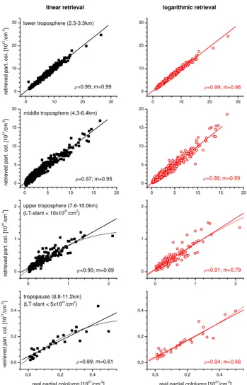
The better performance of the logarithmic approach be-comes visible in Fig. 6, which shows the real characteristics of the correlations for four different layers representing the lower troposphere (LT, 2.3–3.3 km), the middle troposphere (MT, 4.3–6.4 km), the upper troposphere (UT, 7.6–10 km), and the tropopause region (8.8–11.2 km). Depicted are all single ensemble members and curves of linear least squares fits (solid lines) and second order polynomial least squares fits (dotted lines). The correlation coefficient (ρ) and the slope (m) of the regression line are given in the panels. The left panels show the linear and the right panels the logarith-mic retrievals. Above≈6 km the linear retrieval regression

0 10 20 30 0

10 20 30

0 10 20 30 0

10 20 30

0 5 10 15 20 0

5 10 15 20

0 5 10 15 20 0

5 10 15 20

0 1 2

0,0 0,2 0,4 0,0

0,2 0,4

0,0 0,2 0,4 0,0

0,2 0,4

ρ=0.99; m=0.99

retrieved part. col. [10

21/cm -2]

lower troposphere (2.3-3.3km)

ρ=0.99; m=0.96

ρ=0.97; m=0.95

21/cm -2]

middle troposphere (4.3-6.4km)

ρ=0.98; m=0.99

ρ=0.90; m=0.69

21/cm -2]

upper troposphere (7.6-10.0km) (LT-slant < 10x1021

/cm2 )

ρ=0.91; m=0.79

ρ=0.89; m=0.61

21/cm -2]

real partial cololumn [1021 /cm-2

] tropopause (8.8-11.2km) (LT-slant < 5x1021

/cm2 )

ρ=0.94; m=0.66

real partial cololumn [1021 /cm-2

]

Fig. 6.Correlations between assumed real partial column amounts

and their corresponding retrieved amounts in the absence of parameter errors. From the top to the bottom: lower tro-posphere, middle trotro-posphere, upper troposphere (for the LT slant<10_×1021 cm−2sub-ensemble), and tropopause region (for the LT slant<5×1021 cm−2 sub-ensemble). Left panels, black squares and black lines: retrieval on a linear scale and correspond-ing least squares fits. Right panels, red circles: retrieval on a log-arithmic scale and corresponding regression line. Solid lines: lin-ear least squares fit. Dotted lines: second order polynomial least squares fit.

(8)

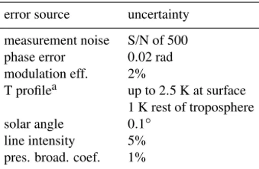
Table 1.Assumed uncertainties.

error source uncertainty

measurement noise S/N of 500 phase error 0.02 rad modulation eff. 2%

T profilea up to 2.5 K at surface 1 K rest of troposphere solar angle 0.1◦

line intensity 5% pres. broad. coef. 1%

a_{detailed description see text}

value. For a better description of this systematic behavior a second order polynomial would be needed. This additional characteristic of the linear retrieval’s smoothing error has im-portant consequences: it limits the linear retrieval in correctly detecting variabilities present in time series. It underesti-mates alterations towards large amounts and overestimate al-terations towards small amounts. For an analysis of water vapour time series above 6 km the logarithmic retrieval is the better choice!

3.2 Model parameter error

As for the smoothing error, the random and systematic errors caused by parameter uncertainties are separated by means of least squares fits. Therefore, the retrievals of spectra simu-lated with correct parameters are corresimu-lated to the retrievals of spectra simulated with erroneous parameters. In this sub-section, errors due to measurement noise, uncertainties in so-lar angle, instrumental line shape (ILS: modulation efficiency and phase error Hase et al., 1999), temperature profile, and spectroscopic parameters (line intensity and pressure broad-ening coefficient) are estimated. The assumed parameter un-certainties are listed in Table 1. Two sources are consid-ered as errors in the temperature profile: first, the measure-ment uncertainty of the sonde, which is assumed to be 0.5 K throughout the whole troposphere and to have no interlevel correlations. Second, the temporal differences between the FTIR and the sonde’s temperature measurements, which are estimated to be 1.5 K at the surface and 0.5 K in the rest of the troposphere, with 5 km correlation length for the inter-level correlations.

Random errors due to measurement noise, uncertainties in the modulation efficiencies, the solar angle and the line inten-sity are situated below or around 5%. They may be neglected if compared to the errors caused by phase error, temperature profile, or pressure broadening coefficient uncertainties. Fig-ure 7 shows the latter errors for the whole ensemble (upper panels) and for the sub-ensembles with low LT slant columns (middle and lower panels). It should be remarked that, owing to the aforementioned nonlinearity ofGˆ, it is impossible to

5 10

0 50 100

5 10

0 50 100

5 10

0 50 100

5 10

0 50 100

5 10

0 50 100

5 10

0 50 100

L

T

slan

t <

5x10

21cm -2 L

T

slan

t <

10x10

21cm -2 w

h

o

le en

sem

b

le

noise/signal [%]

a

ltitu

d

e

[k

m

] pressure broadening phase error T profile (no retr. of T)

T profile (simultaneaous retrieval of T)

noise/signal [%]

al

ti

tude [

k

m]

noise/signal [%]

al

ti

tude [

k

m]

noise/signal [%]

Fig. 7. Parameter errors in the retrieved profiles. Upper

panels: for the whole ensemble. Middle panels: for the LT slant<10_×1021 cm−2 sub-ensemble Bottom panels: for LT slant<5×1021cm−2sub-ensemble. Left panels: linear retrieval. Right panels: logarithmic retrieval. Symbols as described in the legend.

separate the parameter errors completely from the smoothing errors. As a consequence, even systematic error sources may produce random errors (line intensity and pressure broaden-ing parameter). Furthermore, the correlation plots are ex-pected to show some of the characteristics of the smoothing error: e.g. above 6 km the linear retrieval’s sensitivity to-wards parameter uncertainties is expected to be smaller at large amounts than at small amounts. This is the main reason for the linear retrieval’s high random errors above 6 km for the LT slant<5_×1021cm−2sub-ensemble caused by the un-certainties in the phase error parameter. The corresponding errors of the logarithmic retrieval are smaller (at least for the MT and UT).

(9)

This is due to the retrieval’s misinterpretation of spectral sig-natures arising from errors in the temperature profile. Since

ˆ

GKˆpfrom Eq. (6) is generally not equal to zero, the

parame-ter error in the measurement space may be transformed into the state space. This is a minor problem when the minimi-sation of the cost function (Eq. 3) is performed on a linear scale. Then changes of the state vector with respect to its a-priori state and the magnitude of the constraining term are linearly correlated. A misinterpretation would thus mean a large value of the constraining term and consequently Eq. (3) would never be minimised. On a logarithmic scale, however, a linear increase of the constraining term is related to an ex-ponential increase of the retransformed state vector. Hence, a significant change of the state vector is not avoided by the constraining term. The problem can be reduced by a simul-taneous retrieval of the temperature profile, which adds two terms to the cost function:

σ−2(y₋Kx)T(y₋Kx)₊(x₋xa)TSa−1(x−xa)

+σ−2(y₋Ktt)T(y−Ktt)+(t−ta)TSǫt−1(t−ta) (10)

Heretandtaare the real and the assumed temperature state vector,Ktthe sensitivity (or Jacobian) matrix for the

temper-ature, andSǫt the error covariance matrix for the

tempera-ture. Thus a temperature error does not lead to an adjustment of the first term – a misinterpretation of spectral information –, but to an adjustment of the third term in Eq. (10). This reduces the probability of misinterpreting the temperature er-ror. At 6.5 km, for example, the simultaneous fitting of the temperature profile reduces the error from 44% to 13%. This is seen by comparing the red crosses with the red squares in Fig. 7. This strategy leaves the uncertainty in phase error and pressure broadening coefficient as the most important error sources.

For the LT slant<10×1021 cm−2 sub-ensemble (middle panels of Fig. 7), the errors are much smaller (generally be-low 30%). Except for the phase error, the errors for the linear and logarithmic retrieval are now similar. A misinterpreta-tion of spectral signatures is less probable for this ensemble. Apparently, the condition of unsaturated absorption lines si-multaneously eliminates days predestined for misinterpreta-tion. However, a simultaneous retrieval of the temperature further improves the retrievals by reducing the temperature error to below 10% at all altitudes. The most important er-rors are due to uncertainties in the phase error.

The lower panel of Fig. 7 depicts the errors for the LT slant<5×1021 cm−2sub-ensemble. This condition further reduces all errors at altitudes above 5 km. A simultaneous fit of the temperature limits all errors for the logarithmic re-trieval to below 10%. The only exception is the error ow-ing to phase error uncertainties. It still reaches 18% around 10 km.

3.3 Total random errors

Due to the strong non-linearity ofGˆ, the total error cannot be deduced from the smoothing and parameter errors presented above. It has to be simulated separately by a full treatment. Figure 8 shows the correlation matrices for consideration of parameter errors according to Table 1 and for retrievals with-out simultaneous fitting of the temperature profile. It is the same as Fig. 4 but in the presence of parameter errors. The matrices for the whole ensemble (upper panels) show that the parameter errors reduce the sensitivity of both retrievals in the middle and upper troposphere. Additionally, the log-arithmic retrieval performs poorly in the lower troposphere. For the low LT slant sub-ensembles (middle and lower pan-els), the differences to Fig. 4 are much smaller: The param-eter errors are much more important for saturated than for unsaturated absorption lines, which was already observed in Fig. 7.

The total errors for this kind of retrieval are depicted in Fig. 9. If the whole ensemble is considered (black squares) even the retrieval of the 6.4–8.8 km layer becomes uncer-tain (noise/signal of 62% and 75% for the linear and log-arithmic retrieval). For the loglog-arithmic retrieval the large error in the lower troposphere also stands out. For the LT slant<10×1021 cm−2 sub-ensemble, the error in the 6.4– 8.8 km layer is reduced to 45% and the retrieval of the 7.6– 10 km layer is possible with an uncertainty of 53%. The condition of LT slant<5_×1021cm−2further reduces the er-rors: the logarithmic retrieval enables the 8.8–11.2 km layer to be retrieved with an error of only 43%. This realistic error scenario suggests that, considering the whole ensemble, the linear retrieval performs better.

The reason for the poorer performance of the logarithmic retrieval is due to the misinterpretations of spectral signatures as discussed above. There it was shown that the misinterpre-tation of a temperature error is strongly reduced by simulta-neously fitting this parameter. Figures 10 and 11 show that this strategy is also successful concerning the total error. For the logarithmic retrieval the respective correlation matrices (Fig. 10) are very similar to those without additional parame-ter errors (Fig. 4). It should now be possible to retrieve waparame-ter vapour amounts up to at least 7–8 km under all conditions. Figure 11 demonstrates that, for a realistic error scenario and a simultaneous fit of temperature, both linear and logarithmic retrieval yield similar random errors. Considering the whole ensemble, LT and MT amounts can be determined with an acceptable noise to signal ratio of around 22%.

(10)

cor-5 10 15 5

10 15

re

tr

ie

ved atm

o

spher

e [km

]

-0.64 -0.52 -0.40 0.40 0.52 0.64 0.76 0.88 1.00

5 10 15

L

T

slan

t <

5x10

21 cm -2 L

T

slan

t <

10x10

21 cm -2 w

h

o

le en

sem

b

le

re

tr

ie

ved atm

o

spher

e [km

]

-0.64 -0.52 -0.40 0.40 0.52 0.64 0.76 0.88 1.00

5 10 15

re

tr

ie

ved atm

o

spher

e [km

]

-0.64 -0.52 -0.40 0.40 0.52 0.64 0.76 0.88 1.00

5 10 15

re

tr

ie

ved atm

o

spher

e [km

]

-0.64 -0.52 -0.40 0.40 0.52 0.64 0.76 0.88 1.00

5 10 15

re

tr

ie

ved atm

o

spher

e [km

]

-0.64 -0.52 -0.40 0.40 0.52 0.64 0.76 0.88 1.00

5 10 15

re

tr

ie

ved atm

o

spher

e [km

]

-0.64 -0.52 -0.40 0.40 0.52 0.64 0.76 0.88 1.00

Fig. 8.Same as Fig. 4 but in the presence of parameter error as listed in Table 1.

relation with the real amounts at all altitudes, which finally results in higher sensitivity (higher values of slopes), for al-titudes above 6 km, if compared to the linear retrieval. 3.4 Systematic errors

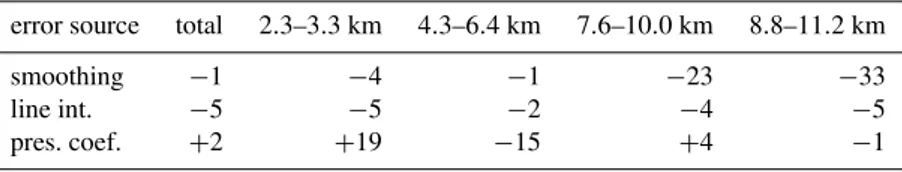
Already in Sect. 3.1, compared to the logarithmic method, the systematic smoothing error of the linear method is shown to be larger. At the same time the linear retrieval’s error

(11)

Table 2. Estimated noise/signal of linear retrieval with simultaneous fitting of temperature [%]. The values for the 7.6–10.0 km and 8.8– 11.2 km layers are for the LT slant<10×1021cm−2and LT slant<5×1021cm−2sub-ensembles, respectively.

error source total 2.3–3.3 km 4.3–6.4 km 7.6–10.0 km 8.8–11.2 km

smoothing 3 14 23 44 45

meas. noise <1 3 2 8 9

pha. err. 2 12 8 24 18

mod eff. <1 1 <1 <1 2

T. profile 1 4 2 6 5

solar angle <1 1 <1 <1 1

line int. <1 <1 <1 2 1

pres. coef. 1 7 7 7 5

total 4 21 24 50 47

Table 3.Same as Table 2, but for logarithmic retrieval.

smoothing 2 10 21 44 36

meas. noise 1 4 2 7 8

pha. err. 2 19 10 33 18

mod eff. <1 1 <1 <1 <1

T. profile 1 8 6 7 3

solar angle 1 <1 <1 <1 <1

line int. <1 1 1 1 1

pres. coef. 1 11 6 5 4

total 4 22 24 49 42

5 10

0 50 100

5 10

0 50 100

noise/signal [%]

a

ltitu

d

e

[k

m

]

whole ens. LT slant <10x1021

cm-2 LT slant <5x1021

cm-2

noise/signal [%]

Fig. 9. Same as Fig. 5 but in the presence of parameter error as

listed in Table 1.

variance of the linear retrieval’s regression line (σ_reg2 ) agrees less well with the real variance. According to Eq. (9) and sinceρ2₌σ_reg2 /σ2

ˆ

x is similar for both retrieval methods, the

absolute variance of the scattering around the regression line (the random error) is then larger for the logarithmic retrieval. However, this is a mean value for the whole ensemble. A detailed analysis would reveal that the linear retrieval has in-creased absolute systematic errors and reduced absolute ran-dom errors only for large amounts. It is vice versa for small

amounts: the absolute systematic errors are increased and the random errors reduced. This once again manifests the dependency of the linear retrieval’s errors on the retrieved amounts. On the other hand, the absolute errors of the log-arithmic retrieval are practically independent from the re-trieved amounts.

Additionally, systematic uncertainties of the spectroscopic line parameters may cause systematic errors. To estimate them, the retrievals of spectra simulated with correct param-eters are linearly correlated to the retrievals of spectra sim-ulated with erroneous parameters. The systematic errors are given as the difference of the regression line slope to unity.

(12)

system-5 10 15 5

10 15

re

tr

ie

ved atm

o

spher

e [km

]

-0.64 -0.52 -0.40 0.40 0.52 0.64 0.76 0.88 1.00

5 10 15

L

T

slan

t <

5x10

21 cm -2 L

T

slan

t <

10x10

21 cm -2 w

h

o

le en

sem

b

le

re

tr

ie

ved atm

o

spher

e [km

]

-0.64 -0.52 -0.40 0.40 0.52 0.64 0.76 0.88 1.00

5 10 15

re

tr

ie

ved atm

o

spher

e [km

]

-0.64 -0.52 -0.40 0.40 0.52 0.64 0.76 0.88 1.00

5 10 15

re

tr

ie

ved atm

o

spher

e [km

]

-0.64 -0.52 -0.40 0.40 0.52 0.64 0.76 0.88 1.00

5 10 15

re

tr

ie

ved atm

o

spher

e [km

]

-0.64 -0.52 -0.40 0.40 0.52 0.64 0.76 0.88 1.00

5 10 15

re

tr

ie

ved atm

o

spher

e [km

]

-0.64 -0.52 -0.40 0.40 0.52 0.64 0.76 0.88 1.00

Fig. 10.Same as Fig. 8 but with simultaneous retrieval of temperature profile.

Table 4. Estimated systematic errors of linear retrieval [%]. The values for the 7.6–10.0 km and 8.8–11.2 km layers are for the LT

slant<10×1021cm−2and LT slant<5×1021cm−2sub-ensembles, respectively.

smoothing 0 ₋3 ₋6 ₋31 ₋38

line int. −5 −5 −3 −3 −4

(13)

Table 5.Same as Table 4, but for logarithmic retrieval.

smoothing −1 −4 −1 −23 −33

line int. ₋5 ₋5 ₋2 ₋4 ₋5

pres. coef. +2 +19 −15 +4 −1

5 10

0 50 100

5 10

0 50 100

noise/signal [%]

a

ltitu

d

e

[k

m

]

whole ens. LT slant <10x1021

cm-2 LT slant <5x1021cm-2

noise/signal [%]

Fig. 11.Same as Fig. 9 but with simultaneous retrieval of

tempera-ture profile.

atic line intensity error, since the increasing sensitivity of the linear retrieval for high amounts reduces the slope of the re-gression line. The same can be observed for the pressure coefficient error: at high altitudes the linear retrieval’s error always lies below the logarithmic retrieval’s error.

3.5 Characterisation of posterior ensembles

On a logarithmic scale all involved pdfs are Gaussian distri-butions. A correctly working retrieval should therefore pro-duce a normal pdf for the posterior ensemble, or if referred to the retransformed linear scale, a log-normal pdf. It should not change the principle distribution characteristics of the a-priori ensemble. The situation of the linear retrieval is differ-ent because it involves normal and log-normal pdfs. Conse-quently the posterior pdf may be something between a log-normal and log-normal pdf. Aχ2test can check this issue. The posterior covariance matrix isSx_ˆ=ǫ{xˆxˆT}. In contrast to the

a-priori covariance matrixSa, the matrixSx_ˆis singular, since

the solution space has fewer dimensions than the a-priori space. The calculation of theχ2values according to Eq. (5) is thus not straightforward. However, since the covariance matrix is symmetric its singular value decomposition leads toL3LT, with the columns ofLcontaining its eigenvectors and the diagonal matrix3its corresponding eigenvalues. As

S−1in Eq. (5) a pseudo inverse is applied, which only con-siders the 3 largest eigenvalues. Theχ2calculated with this inverse would thus have 3 degrees of freedom. The test is performed for all aforementioned retrievals: with/without pa-rameter errors and with/without simultaneous fitting of

tem-0 10 20 30 0

10 20 30

0 10 20 30 0

10 20 30

0 5 10 15 20 0

5 10 15 20

0 5 10 15 20 0

5 10 15 20

0 1 2

0,0 0,2 0,4 0,0

0,2 0,4

0,0 0,2 0,4 0,0

0,2 0,4

ρ=0.98; m=0.98

21/cm -2]

ρ=0.98; m=0.98

ρ=0.97; m=0.83

21/cm -2]

ρ=0.97; m=0.86

ρ=0.87; m=0.55

21/cm

-2] upper troposphere (7.6-10.0km) (LT-slant < 10x1021

/cm2 )

ρ=0.87; m=0.64

ρ=0.88; m=0.53

21/cm -2]

real partial column [1021 /cm-2

/cm2 )

ρ=0.91; m=0.62

real partial column [1021 /cm-2

]

Fig. 12.Same as Fig. 6 but in the presence of parameter errors and

with simultaneous retrieval of temperature profile.

(14)

2 3 4 5 6 7 8 9 10 40

60 80 95

2 3 4 5 6 7 8 9 10

40 60 80 95

2 3 4 5 6 7 8 9 10

40 60 80 95

theoretical χ2_cdf

empirical χ2

cdfs: without parameter errors with parameter errors, but no temp. retrieval

with parameter errors and sim. temp. retrieval

probabilit

y

[

%

]

χ2

test not possible due to occasionally

negative mixing ratios with linear

retrieval !

probabilit

y

[

%

]

χ2

χχχχ

2 t

est

f

o

r lo

g

-n

o

rm

a

l d

ist

rib

u

tio

n

χχχχ

2 t

e

s

t f

or

nor

m

a

l di

s

tr

ibut

ion

probabilit

y

[

%

]

χ2

Fig. 13. χ2 test for posterior ensembles. Upper panels: χ2test

assuming normal distribution. Lower panels:χ2test assuming normal distribution. Left panels: linear retrieval. Right panels: log-arithmic retrieval. Black line: theoreticalχ2cumulative distribu-tion funcdistribu-tion (cdf) for 3 degrees of freedom; black filled squares: empiricalχ2cdf of ensemble in absence of parameter errors; black circles: empiricalχ2cdf of ensemble in the presence of parameter errors and without retrieval of temperature profile; red circles: em-piricalχ2cdf of ensemble in the presence of parameter errors and simultaneous retrieval of temperature profile.

circles) represent the posterior ensemble when no parameter errors are assumed. The linear posterior ensemble is quite consistent with a normal distribution. This means that the linear retrieval forces the originally log-normally distributed ensemble into a Gaussian ensemble. Additional errors push the solutions slightly away from a normal distribution. A simultaneous retrieval of the temperature enables a better ex-ploitation of the information present in the spectra and leads nearly to the same distribution characteristic as if no errors were present. The logarithmic posterior ensemble has fewer characteristics of a normal distribution. Its empiricalχ2cdfs differ considerably from the theoreticalχ2cdf. The lower panel checks for a log-normal distribution. This test cannot be performed for the linear retrieval since it yields occasion-ally to negative retrieved values. In the absence of parameter errors, the logarithmic retrieval does not change the charac-teristics of the a-priori distribution. It is still a log-normal distribution (black squares). The presence of parameter er-rors pushes the posterior ensemble slightly away from a pure log-normal distribution (black and red circles).

2 3

no temperature retrieval

DOF (

real

is

ti

c er

ro

rs

)

DOF (no parameter error)

simultaneous temperature retrieval

DOF (

real

is

ti

c er

ro

rs

)

DOF (no parameter error)

Fig. 14. DOF values for logarithmic retrievals with realistic error

assumptions compared to DOF values of logarithmic retrieval in the absence of errors. Left panel: no retrieval of temperature profile. Right panel: simultaneous retrieval of temperature profile.

In the case of misinterpretation of spectral signatures the logarithmic retrieval over-interprets spectral signatures. This can be demonstrated by analysing the trace of the averaging kernel matrix (tr(Aˆ)). It determines the amount of informa-tion present in the spectra used by the retrieval for updat-ing the a-priori state. It is commonly called the degree of freedom of the measurement (DOF). Figure 14 compares the DOF values for the logarithmic retrievals with and without additional errors. If the retrieval is working correctly adding further errors should reduce the DOF value, since the infor-mation in the spectra is more uncertain. However, on a log-arithmic scale occasionally the contrary is observed. If the temperature profile is not simultaneously fitted (left panel of Fig. 14) occasionally more information is retrieved from the erroneous spectra than from the spectra with only white noise, which means that errors in the spectra are misinter-preted as information. This problem disappears by fitting the temperature profile simultaneously (right panel).

4 Comparison of retrieval results to ptu-sonde

measure-ments

4.1 The FTIR measurements

(15)

applied whose nonlinearities were corrected. The spectra are typically constructed by co-adding up to 8 scans recorded in about 10 or 13 min, depending on their resolution. Analysing the shape of the absorption lines (lines are widened by pres-sure broadening) and their different temperature sensitivities enables the retrieval of the absorbers’ vertical distribution. Since the instrumental line shape (ILS) also affects the shape of the measured absorption lines, this instrumental charac-teristic should be determined independently from the atmo-spheric measurements. This is done on average every two months using cell measurements and LINEFIT software as described in Hase et al. (1999). The temperature and pres-sure profiles, necessary for the inversion, are taken from the synoptical meteorological 12:00 UT sondes. Above 30 km data from the Goddard Space Flight Center’s automailer sys-tem are applied. Some results of these measurements are presented in Schneider et al. (2005) and references therein. 4.2 The radiosonde measurements

Until September 2002 the meteorological soundings were launched from Santa Cruz de Tenerife, 35 km northeast of the observatory, and since October 2002 in an automised mode from G¨uimar, 15 km southeast of the observatory. The son-des are equipped with a Vaisala RS80-A thin-film capaci-tive sensor which determines relacapaci-tive humidity. The sonde data are corrected by a method suggested by Leiterer et al. (2004), who reported a remaining random error of less than 5% throughout the troposphere. Other authors report cor-rection methods with a remaining uncertainty of over 10% (Miloshevich, 2001). Furthermore, the precision of the wa-ter vapour measured by the RS80-A sensor may be degraded due to chemical contamination during storage. To avoid son-des with iced detectors, sonson-des that passed through clouds are not taken into account. Therefore sondes which detect a vapour pressure close to the liquid or ice saturation pres-sure are disregarded. Furthermore, sondes with unrealistic high humidities above 10 km, which may indicate an iced detector, are excluded. The corrected sonde mixing ratios are finally sampled on the altitude grid of the retrieval by re-quiring that linear interpolation of the mixing ratios between two grid levels yield the same partial columns as the original highly-resolved data.

4.3 Temporal and spatial variability

The large temporal and spatial variabilities of atmospheric water vapour are problematic when measurements conducted from different platforms are to be compared. Both experi-ments should be conducted at the same time and sound the same atmospheric location. For this reason only sonde mea-surements coinciding within 2 h of the FTIR meamea-surements are used for the comparison. Spatial coincidence is difficult to achieve. The sonde measures in-situ and will always be situated at a certain distance from the imaginary line between

the FTIR instrument and the sun. This is particularly prob-lematic for the lowest layer above the FTIR instrument as, while the FTIR instrument is located at the surface the sonde is typically floating around 30 km south of the observatory in the free troposphere. A comparison between the humidity measured in-situ at the observatory and the sonde’s humidity demonstrated that the water vapour amounts close to the sur-face are more variable and on average 40% larger than those in the free troposphere.

4.4 Comparison

(16)

5 10 15 5

10 15

sonde atmosphere [km]

re

tr

ie

ved atm

o

spher

e [km

]

-0.64 -0.52 -0.40 0.40 0.52 0.64 0.76 0.88 1.00

5 10 15

L

T

slan

t <

5x10

21 cm -2 L

T

slan

t <

10x10

21 cm -2 w

h

o

le en

sem

b

le

re

tr

ie

ved atm

o

spher

e [km

]

-0.64 -0.52 -0.40 0.40 0.52 0.64 0.76 0.88 1.00

5 10 15

re

tr

ie

ved atm

o

spher

e [km

]

-0.64 -0.52 -0.40 0.40 0.52 0.64 0.76 0.88 1.00

5 10 15

re

tr

ie

ved atm

o

spher

e [km

]

-0.64 -0.52 -0.40 0.40 0.52 0.64 0.76 0.88 1.00

5 10 15

re

tr

ie

ved atm

o

spher

e [km

]

-0.64 -0.52 -0.40 0.40 0.52 0.64 0.76 0.88 1.00

5 10 15

re

tr

ie

ved atm

o

spher

e [km

]

-0.64 -0.52 -0.40 0.40 0.52 0.64 0.76 0.88 1.00

Fig. 15.Same as Fig. 10 but for correlation matrices between measured sonde and FTIR profiles.

retrieval at high altitudes if compared to the linear retrieval. Tables 6 and 7 list these differences. They are calculated from least squares fits as described in section 3.1. The dif-ference to unity of the slope gives the systematic deviation and the scattering around the regression line gives the ran-dom deviation. This scattering describes the level of consis-tency between the variabilities detected by the sonde and the FTIR measurements. It may also be seen as the overall pre-cision of FTIR and sonde experiments together. For the UT and tropopause layer and considering the coincidences with

(17)

Table 6. Differences between sonde and FTIR column amounts as estimated from the correlation plots (Fig. 16). The values for the 7.6– 10.0 km and 8.8–11.2 km layers are for the LT slant<10×1021cm−2and LT slant<5×1021cm−2sub-ensembles, respectively.

total 2.3–3.3 km 4.3–6.4 km 7.6–10.0 km 8.8–11.2 km

random 25 40 32 54 56

systematic +6 +3 −4 −40 −47

Table 7.Same as Table 6 but for logarithmic retrieval.

total 2.3–3.3 km 4.3–6.4 km 7.6–10.0 km 8.8–11.2 km

random 25 47 33 58 51

systematic ₊6 ₋4 ₊1 ₊2 ₋10

An outstanding difference to Tables 2 and 3 is the poorer consistency for the LT layer of FTIR when compared to sonde than when compared within the simulations: empir-ical standard deviation of≈45% compared to the estimated values of below 22%. This is due to the aforementioned dif-ferent conditions in the lowermost layer above the instrument (surface influences) and the corresponding layer at the sonde (free troposphere). Since the LT mainly determines the to-tal column amount, the latter is also largely affected by these differences. The estimated and empirically observed preci-sion for the MT are much more consistent: estimated noise to signal for the FTIR of 24% versus measured≈32% for both experiments together.

Figure 16 shows the correlation between LT, MT, UT, and tropopause partial column amounts of FTIR and sonde mea-surements. The greatest differences with Fig. 12 are ob-served for the LT (as discussed above), where the regres-sion line between sonde and FTIR data has on offset of

≈2.5×1021 cm−2: the LT at the site of the instrument is more humid than the free tropospheric LT. For the MT the consistency between the simulations and the empirical ob-servations is excellent, even though the errors of the sonde measurements and temporal and spatial mismatching are still disregarded. The regression lines for the UT and the tropopause region show a small offset. Retrieved amounts are≈1×1020cm−2larger than the sonde amounts. This may confirm a dry bias of the sonde measurements (Turner et al., 2003). The slopes of the linear regression lines for the UT and tropopause region are 1.02 and 0.90 for the logarithmic retrieval. These values are much larger than the simulated slopes of 0.64 and 0.62. The reason may be that the humidity applied for the first layer in the simulations differs from the real humidity of this layer. Due to the aforementioned differ-ent condition at the sonde and at instrumdiffer-ent altitude (2.3 km), a mixing ratio determined by an in-situ instrument was ap-plied for the simulation. This relatively high value is then spread out up to the next grid point (3.3 km). However, the

enhanced humidity due to surface conditions is very likely limited to the lowest 100 m of the atmosphere. This overesti-mation of simulated LT amounts reduces the mean estimated sensitivity in the UT and tropopause region.

Figure 16 further demonstrates that the logarithmic re-trieval is correlated linearly to the sonde data at all altitudes, whereby for high altitudes the linear retrieval’s regression line underestimates both especially large and small amounts. This is consistent with the simulations (Fig. 12). The experi-ments confirm that at high altitudes the linear retrieval is less sensitive at large amounts if compared to small amounts. The empirical validation suggests that the differences between the linear and logarithmic retrievals’ systematic errors are even more pronounced than proposed by the theoretical study per-formed in Sect. 3. This is reflected in the larger differences between the slopes of the regression lines for the linear and logarithmic retrieval. While at higher altitudes and for days with low LT slant column amounts, slopes of around 0.53 for the linear retrieval versus 0.63 for the logarithmic retrieval are simulated, the empirical validation yields 0.57 versus 0.96. An explication may be that the assumed measurement noise is underestimated in the simulations, since all spectra were calculated for no aerosol loading. More measurement noise would mean that the a-priori information is more im-portant and, since the linear retrieval applies a wrong a-priori, the caused systematic error would increase.

(18)

0 10 20 30 0

10 20 30

0 10 20 30 0

10 20 30

0 5 10 15 20 0

5 10 15 20

0 5 10 15 20 0

5 10 15 20

0 1 2

0,0 0,2 0,4 0,6 0,0

0,2 0,4 0,6

0,0 0,2 0,4 0,6 0,0

0,2 0,4 0,6

ρ=0.91; m=1.03

21/cm -2]

ρ=0.88; m=0.96

ρ=0.95; m=0.96

21/cm -2]

ρ=0.94; m=1.01

ρ=0.81; m=0.60

21/cm -2]

upper troposphere (7.6-10.0km) (LT-slant < 10x1021

/cm2 and S/N > 200)

ρ=0.81; m=1.02

ρ=0.83; m=0.53

21/cm -2]

sonde partial column [1021 /cm-2

/cm2 and S/N > 200)

ρ=0.86; m=0.90

sonde partial column [1021 /cm-2

]

Fig. 16.Same as Fig. 12 but for measured sonde and FTIR partial

column amounts.

5 Subtropical water vapour time series

Figure 17 depicts a nearly 7 year record of tropospheric wa-ter vapour amounts as dewa-termined by the logarithmic retrieval with simultaneous fitting of the temperature. The black cir-cles show data from the Bruker IFS 120M, which was op-erated until April 2005. The red crosses are results as ob-tained from a Bruker 125HR, which measures since Jan-uary 2005. While for the lower and middle tropospheric values all measurement days are depicted, the upper tropo-spheric and tropopause values are presented only when the LT slant column amounts are lower than 10_×1021cm−2and 5×1021cm−2, respectively. For the lower and middle tropo-sphere a well pronounced seasonal cycle is observed. Val-ues are highest at the end of summer and lowest in the win-ter months. A similar clear seasonal dependence is not ob-served for the upper tropospheric amounts and the amounts of the tropopause region. Values are sometimes even espe-cially high in autumn/winter, which demonstrates their

inde-pendence from lower tropospheric levels. A quick view may give the impression of increasing water vapour contents in the upper troposphere; however, for a serious trend analysis a longer and more continuous time series would be needed.

6 Summary and conclusions

Compared to other atmospheric components, the retrieval of atmospheric water vapour from ground-based FTIR mea-surements has additional difficulties. Water vapour has very large vertical gradients and variabilities, which generally limit the sensitivity of the ground-based technique to the lower and middle troposphere. The spectral signatures orig-inating from the upper troposphere are rather weak and thus their retrieved values depend to an important extent on a-priori assumptions. Water vapour mixing ratios are log-normally distributed and an inversion on a logarithmic scale enables the correct application of this a-prior knowledge and consequently leads to a statistically optimal retrieval. How-ever, this method introduces the risk of misinterpreting spec-tral signatures produced by errors in assumed model parame-ters. It is shown that the misinterpretations can be controlled by simultaneously fitting the temperature profile. A logarith-mic retrieval should therefore perform better than the com-monly applied linear retrieval, in particular for high altitudes where the spectral signatures are similar to the measurement noise. It is found that the linear retrieval leads to large sys-tematic errors, which are difficult to characterise. They can be observed in correlation plots between retrieved and real amounts. The complex character of the linear retrieval’s systematic error has important consequences: it limits the linear retrieval in correctly detecting variabilities present in time series. It would underestimate alterations towards large amounts and overestimate alterations towards small amounts. The systematic error of the logarithmic retrieval is smaller. Its amounts are almost linearly correlated to the real amounts, i.e. its sensitivity is independent from the retrieved amount. For an analysis of water vapour time series of the upper tro-posphere and the tropopause region the logarithmic retrieval has to be applied. A realistic error scenario simulates ran-dom errors of 4% for the total column amounts and around 23% for amounts of the lower and middle troposphere. On days with low LT slant amounts, amounts of the upper tro-pospheric and the tropopause region can also be determined with an uncertainty of around 45%. Furthermore, it is found that, in addition to the limited vertical resolution, the uncer-tainties in the instrumental line shape (phase error) are re-sponsible for the most important errors. All these estimations are confirmed by a comparison to sonde measurements.