Multiuser CoMP transmit processing with statistical
channel state information at the transmitter
Lígia Ma. C. Sousa, Tarcisio F. Maciel, and Charles C. Cavalcante
Wireless Telecom Research Group - GTEL, Federal University of Ceará,CP 6005, Campus do Pici,60455-760, Fortaleza, Brazil, {ligia, maciel, charles}@gtel.ufc.br
Abstract—Coordinated Multi-Point (CoMP) transmis-sion/reception is a candidate technique for increasing cell-average and cell-edge throughputs in next-generation wireless systems. Joint Processing (JP) can enhance CoMP systems’ performance, mainly employing precoding algorithms based on channel state information at the transmitter (CSIT). Currently, many research efforts focus on reducing feedback and optimizing precoding with partial CSIT. This paper proposes a model to approximate the downlink multiuser CoMP channel based on the channel statistics and taking into account the channel temporal variation. The proposed model is relatively simple, highly reduces feedback overheads, and might be employed to perform precoding. Compared to using linear precoding with instantaneous CSIT, results show that throughput losses are negligible for low SNR values and moderate for high SNR values when using the proposed model. Analyses considering users all over the cell and in the cell-edge are also presented.
I. INTRODUCTION
Coordinated Multi-Point (CoMP) transmission/reception has been considered as a promising approach to improve coverage with high data rates and cell-edge throughput [1]. CoMP trans-mission can be categorized into two classes: Joint Processing (JP), where data are simultaneously transmitted from multiple transmission points to a single user as to improve its received signal quality and/or actively cancel interference from other users; and Coordinated Scheduling/Beamforming (CS/CB), in which data is only available at the serving cell (data transmission from that point) but user scheduling/beamforming decisions are made with coordination among cells belonging to the CoMP cooperating set [1].
The benefits of Multiple-Input-Multiple-Output (MIMO) systems are enhanced when the transmitter exploits channel state information (CSI) to process, in an intelligent way, the signal before transmission. This can be accomplished by pre-coding techniques, which often rely on the assumption that the transmitter knows perfectly the MIMO channel matrix [2], [3]. However, this may not be realistic in many practical scenarios and considering partial availability of CSIT in MIMO systems becomes an important issue. This assumption might have a significant impact on the throughput that can be reliably obtained by the system.
Partial CSIT was firstly introduced in [4], where Lloyd’s algorithm is used to quantize CSI. Indeed, some limited
feed-This work was partially supported by the Research and Development Cen-ter, Ericsson Telecomunicações S.A., Brazil, under EDB/UFC.25 Technical Cooperation Contract and National Research Council (CNPq), Brazil.
back multiuser MIMO schemes let each user quantize some function of the channel coefficients and feed this information back to the transmitter [5], [6]. Problems occur, e.g., when user signals can not be perfectly orthogonalized by precoding due to channel quantization errors. To avoid this, schemes have been proposed which select, at the receiver, a quantized precoder from a codebook. Then, only the precoder index is fed back to the transmitter [7], [8]. However, designing precoder codebooks is a quite difficult task, which must take into account the statistical characteristics of the channel. Other approaches focused on feeding back the mean [9] or the covariance matrix [10] of the channel, which convey important information about the slow fading and the mean spatial separability of the users. However, such techniques usually do not take into account the temporal variation of the channel, leading to accuracy degradation of CSIT.
In this work, we propose a multicell multiuser dynamic channel model which assumes that the transmitter has only partial channel information, while the receiver has access to instantaneous CSI. This partial information consists of the channel statistics and the temporal correlation parameter. The simulation results show that the proposed channel model plays a significant role in low-SNR regimes in which the transmit power is only sufficient to excite a subset of the eigenmodes of the channel.
The remainder of this paper is organized as follows. In section II, the multicell multiuser MIMO system considering CoMP is presented. In section III we describe our proposal for modeling the CSIT. Simulation results are presented in section IV. Finally, conclusions are stated in section V.
II. SYSTEMMODEL
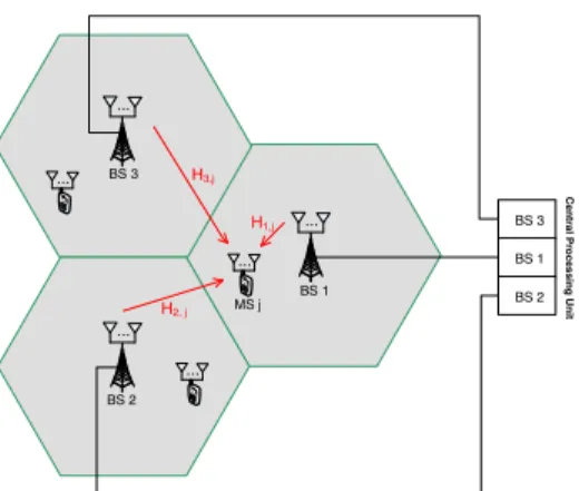
We consider the downlink of a multicell multiuser MIMO communication system composed by �� Base Stations (BSs) and� cochannel Mobile Stations (MS) arbitrarily distributed within the system coverage area. Each BS is equipped with �� transmit antennas and each MS with�� receive antennas. The BSs are connected to a central processing unit, thus characterizing a CoMP structure. Moreover, synchronization among the BSs is assumed. Hereafter (��,��,��,�) will be used to represent the overall structure of the system. Figure 1 shows this representation for a case with ��=�= 3.
BS 2
BS 1 BS 3
... ...
...
...
MS j
... ... H3,j
H2, j
H1,j
BS 2 BS 3
BS 1
Ce
n
tra
l P
ro
ces
si
n
g
U
n
it
Figure 1. Multicell multiuser MIMO system model with��=�= 3.
Rayleigh-distributed small-scale fading is considered, which is modeled using Jake’s model [11]. The spatial channel characteristics assume Kronecker-structured covariances with a transmit covariance matrix Rt� and a receive covariance
matrix Rr� for each MS �. Considering this, the channel
matrix from all BSs to MS � at time�can be modeled as
H�[�] =Rr 1/2
� HJakes[�]Rt 1/2
� , (1)
where H� = [H1,� H2,� . . . H��,�
]
������ is the
joint channel matrix from all BS to MS � with H�,� being the channel matrix from base � to user � and HJakes[�]
is a �� ���� small-scale fading channel matrix. Here, Rt1�/2 is the principal square-root of Rt�, such that,Rt� =
Rt1�/2Rt1�/2. Analogously, Rr�=Rr1�/2Rr1�/2.
As already mentioned, in a CoMP-JP system, the transmit signal intended for each user � is spread over all �� BSs.
It can be expressed as x� =
[
x[1]� � x[2]� � . . . x[��]�
�
]�
,
wherex[��] is the signal transmitted from BS�for user�. The signaly� received at MS � is
y� =H�x�+
∑
�∕=�
H�x�+n�, (2)
where n� is the background noise and time � is omitted for simplicity.
Let�� denote the number of data streams intended for MS �, � = 1,2, . . . , �. For each MS, an ���� ×�� precoder matrix T� is designed based on the characteristics of HΣ�. UsingT�, Equation (2) can be rewritten as
y�=H�Ts+n�, (3)
where T = [
T1 T2 . . . T�]�
����� is the joint
pre-coding matrix,s=[
s�1 s�2 . . . s��]�
��×1is the joint data
stream vector withs� being a data stream intended for MS� and �� =∑�
�=1��. For simplicity, streams are assumed to
have i.i.d. zero-mean unit-variance complex Gaussian entries, i.e., Gaussian signaling is assumed.
In (2), the term ∑
�∕=�HΣ�T�s� represents the asyn-chronous reception by MS � of the signal sent for the MS �,� ∕=�. Since MS� is not interested in correctly detecting s�, the design of the joint transmit matrix T is not affected
by asynchronous receptions of interfering signals and s� can be simply viewed as the data of some virtual synchronous interfering MSs.
III. MULTIUSERMULTICELLDYNAMICCSIT MODEL A. Covariance and Auto-covariance of the Channel
The channel covarianceR�[0]of MS� captures the spatial correlation among all transmit and the receive antennas of MS �being a������������positive semi-definite Hermitian matrix defined as
R�[0] =�{hΣ�h∗Σ�
}
, (4)
where hΣ� =vec(HΣ�), and (.)∗ denotes a conjugate trans-pose. Its diagonal elements represent the power gain of the ������×������ scalar channels from all BSs to MS �, and the off-diagonal elements are the cross-coupling between these scalar channels.
Assuming that R�[0] has the simplified, separable Kro-necker structure [12], it can be decomposed as
R�[0] =Rt��[0]⊗Rr�[0], (5)
where ⊗denotes the Kronecker product. Moreover, assuming stationarity, the auto-covariance between two channel samples HΣ�[�] and HΣ�[�+�] depends on the time difference � but not on the absolute time and is given by
R�[�] =�{hΣ�[�]h∗Σ�[�+�]
}
, (6)
which coincides withR�[0]in (4) when�= 0and eventually decays to zero when �becomes large.
The channel auto-covariance characterizes how fast the channel decorrelates with time. While the covariance R�[0] captures the spatial correlation among all transmit and receive antennas of user �, the channel auto-covariance at a non-zero time differenceR�[�]captures both channel spatial and temporal correlations.
Based on the premise that the channel temporal statistics for all antenna pairs of the same MS � can be the same, the channel gains between all the���� transmit antennas and�� receive antennas of the BSs-MS link have the same temporal correlation function. Then, at each time �, it is possible to separate the temporal correlation ��[�] from the spatial correlationR�[0]and the auto-covarianceR�[�]becomes their product as
R�[�] =��[�]R�[0],with (7)
��[�] =�0(2�����
)
, (8)
where �0(.) is the zero-th order Bessel function of the first
kind and��� is the maximum Doppler spread of MS�at time
� [11] [13].
B. Channel Estimation at the Transmitter
Firstly, we assume that the transmitter has an initial channel measurement at time�= 0and relevant channel statistics for each MS �, namelyH�[0]andR�[0].
considered error-free, the main source of irreducible error in channel estimation will be the channels’ random variation in time. Thus, the error in the channel estimate depends only on the time difference�between this initial measurement and its use by the transmitter.
Let HˆΣ�[�] be the channel estimate for MS � at time � andEΣ�[�]the estimation error with correlationRe�[�]. The
CSIT model can be written as
HΣ�[�] =HˆΣ�[�] +EΣ�[�], (9)
Re�[�] =�{eΣ�[�]eΣ�[�]∗} (10)
whereeΣ�[�] =vec(EΣ�[�]). In the following, we show how the CSIT of each user�, which consists of the estimateHˆΣ�[�] and its error covarianceRe�[�], can be obtained using MMSE
estimation theory.
C. Linear Estimation Theory for the CSIT Problem
Since thehΣ�[�]andhΣ�[0]vectors are dependent random variable vectors, the value assumed byhΣ�[�]can be estimated when the value byhΣ�[0]is known or measured. Indeed, the estimate ˆhΣ�[�] can be described as a function of the value assumed byhΣ�[0], i.e.,
ˆ
h�[�] =�(h�[0]). (11)
The challenge is to suitably choose�(⋅)to yield a reason-able estimatehˆΣ�[�], which means to satisfy a desired opti-mality criterion. Considering the mean square error criterion, it can be shown that the optimum estimate is [14]
ˆ
hΣ�[�] =�{hΣ�[�]∣hΣ�[0]}. (12)
Calculating this expectation requires full knowledge of the joint probability density function of hΣ�[�] and hΣ�[0], which is often hard to obtain. However, if we restrict the estimation function �(⋅) to be a lin-ear function of the observations1, then it turns out that
all we shall need is knowledge of first- and second-order statistics �{hΣ�[�]}, �{hΣ�[0]}, �{hΣ�[�]hΣ�[�]∗},
�{hΣ�[0]hΣ�[0]∗}and�{h
Σ�[�]hΣ�[0]∗}. Thus, the estima-tion funcestima-tion will be given by
ˆ
h�[�] =K�h�[0] (13)
where K� ∈ ℂ������×������ is a coefficient matrix min-imizing the resulting error covariance matrix and which we need to determine.
Since�(K)is the mean square error matrix given by
�(K) =�{(hΣ�[�]−KhΣ�[0])(hΣ�[�]−KhΣ�[0])∗}, (14)
our optimization problem will be
K�= arg min
K
�(K), (15)
which is equivalent to require
a�(K)a∗≥a�(K�)a∗ (16)
for every K and for every row vector a [14]. This change simplifies the optimization problem, sincea�(K)a∗is a scalar
1This restriction is not so hard since whenh
�[�]andh�[0]are jointly
Gaussian, an assumption that is often reasonable, the unconstrained least mean squares estimation function is linear [14].
function of a complex-valued (row) quantity aK, which is more tractable. Thus, K� solves (13) if, and only if, for all vectors a,aK� is a minimum ofa�(K)a∗.
Differentiatinga�(K)a∗with respect toaKand setting the derivative equal to zero atK=K�, i.e.,
∂(a(R�[0]−R�[�]∗K∗−KR�[�] +KR�[0]K∗)a∗) ∂aK
K=K�
= 0
yields
K� =R�[�]∗R−�1[0]. (17)
After some mathematical manipulations on (17), the mini-mum mean square error matrix �(K�)is obtained as
�(K�) =�{(hΣ�[�]−K�hΣ�[0])(hΣ�[�]−K�hΣ�[0])∗}
=R�[0]−R�[�]∗R−1
� [0]R�[�]. (18)
Thus, the CSIT at time � for MS� given by the estimate ˆ
H�[�]and its error covarianceRe�[�] become
ˆ
HΣ�[�] =K�HΣ�[0] =R�[�]∗R−�1[0]HΣ�[0], and (19)
Re�[�] =�(K�) =R�[0]−R�[�]∗R−�1[0]R�[�] (20)
The two quantitiesHˆΣ�[�]andRe�[�]constitute the CSIT.
They effectively function as channel mean and channel covari-ance at time �for MS �.
Using the homogeneous channel temporal correlation as-sumption given in (7), the channel estimate and its error covariance become
ˆ
H�[�] =��[�]H�[0], and (21)
Re�[�] = (
1−��[�]2)
R�[0]. (22)
Thus, the CSIT for each user � is simply characterized as a function of ��[�],H�[0]andR�[0].
From (5), the error covariance Rt�,�[�] can similarly be
decomposed in effective antenna correlations as
Rt�,�[�] = √
1−��[�]2R
t�[0],and
Rr�,�[�] = √
1−��[�]2R r�[0].
(23)
Thus, the channel matrix at time� for MS� is becomes
HΣ�[�] = ˆHΣ�[�] +Rr�,�[�]1/2H�Rt�,�[�]1/2, (24)
where H�is a������ channel matrix whose entries are zero-mean circular symmetric complex Gaussian variables.
In this CSIT model,��[�]acts as a channel estimate quality dependent on the time �. For small � values, ��[�] is close to 1, the estimate depends heavily on the initial channel measurement and the error covariance is small. As�increases, ��[�]decreases, the impact of the initial channel measurement is reduced and the error covariance grows towards the channel covariance R�[0].
IV. SIMULATION ANDRESULTS
A. Scenario, Channel Model and Main Simulation Parameters
For simulation of the multicell multiuser dynamic model, we have the following steps:
1) The covariance matrixR�[0]is measured at the BS based on the pilot symbols sent in uplink by MS�. Due to chan-nel stationarity, R�[0]keeps valid all over the simulation. 2) Blocks of��symbols are considered and, at the beginning of each block, MSs send their initial channel measurement H�[0]to the BS.
3) For each symbol period��, users send their corresponding parameter ��[�] to BSs and the CSIT is estimated using (21), (23) and (24) at the central processing unit. We can note that if the transmitter knows the users’ speed, the parameter�can be evaluated by BSs and it is not needed as feedback.
The most relevant parameters considered in the simulations are shown in table I.
Table I
PARAMETER OF THESIMULATIONS.
Parameters Value
Cell radius 1km
Number of Tx antennas per BS�� 2
Number of Rx antennas per MS�� 2
Carrier Frequency 1.8GHz
System Bandwidth 100kHz
Users velocity 60km/h
Doppler frequency�� 100Hz
Coherence Time 2�1
� = 5ms
Noise power −103dBm
The initial antenna correlations are fixed for all MSs as
Rt�[0] = ⎛
⎝ [
1 0.3 0.3 1
] ⊗
⎡
⎣
1 0 0 0 1 0 0 0 1 ⎤
⎦ ⎞
⎠
��������
andRr�[0] = [
1 0 0 1 ]
����
.
B. Precoding Technique and Power Allocation
For the considered CoMP scenario, power constraints are per BS and for simplification the precoding matrix T is determined in a suboptimal way as follows. First, precoders are determined without considering the per BS power con-straints (yielding unit-norm beamformers) according to ex-istent precoding techniques, namely, Zero Forcing (ZF) and Minimum Mean Square Error (MMSE) [13]. Afterwards the per-BS power constraints are imposed using a power loading matrix, so that we have T = FΩ, where F = [
F1 F2 . . . F�]�
����� is the precoder matrix withF�
representing the precoding matrix for the MS � and Ω the power loading matrix.
The matrixΩ=�Iis an��×�� diagonal matrix with� being the power allocated equally for the original data streams. Then, Ωcan be calculated as
Ω=�I, �= min
�=1,2,⋅⋅⋅,��
⎷ (
�BS_�
F[�]
2
ℱ
)
, (25)
where F[�] contains the rows of F corresponding to the transmit antennas at BS � [15],∥.∥ℱ is the Frobenius norm, and�BS_� is the power constraint of BS�.
C. Performance Metrics
In order to evaluate the simulation results, the average throughput per user TRavgis adopted as performance measure.
It is given by
TRavg= 1
� ���
∑
�=1 log2
(
1 + ∥Heq�,�∥ 2
∑
�∕=�∥Heq�,�∥2+∥n∥2 )
, (26)
where Heq = HT is the product of the channel matrix by
the precoding matrix andHis the channel matrix of all users given by H = [H�Σ1, . . . ,H�Σ�]� and H
eq�,� is the element
of the �-th row and�-th column of the matrix Heq.
D. Results
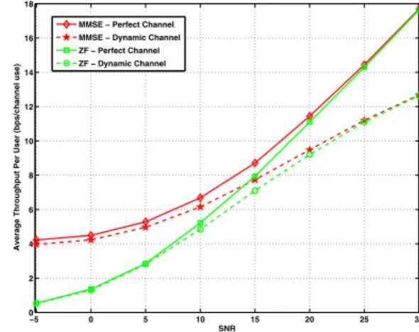
In figure 2, the average throughput using ZF and MMSE precoding considering perfect and dynamic CSIT are com-pared for the scenario (2,2,3,3) with �� = 5 symbols per block. At low SNRs, the performance obtained with the dynamic CSIT model is quite similar to the perfect channel. Only from an SNR value of 15 dB, the performance gap between perfect and dynamic CSIT increases.
−5 0 5 10 15 20 25 30
0 2 4 6 8 10 12 14 16 18
SNR
Average Throughput Per User (bps/channel use)
MMSE − Perfect Channel
MMSE − Dynamic Channel
ZF − Perfect Channel
ZF − Dynamic Channel
Figure 2. Throughput curves for ZF and MMSE precoding using perfect
CSIT and the dynamic CSIT model (��= 5).
The proposed CSIT model has been simulated using pre-coding techniques originally designed for perfect CSIT. Thus, it is interesting to notice the good results obtained with the proposed model even in this non-ideal situation.
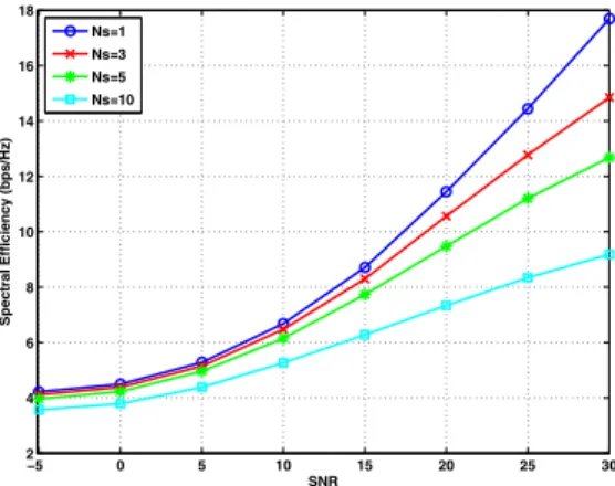
In order to evaluate how the performance of proposed schemes changes when the number�� of symbols per block varies, the previous scenario has been simulated using MMSE precoding for increasing values of��. The obtained through-put results are shown in figure 3. Therein, we can note that the results are similar in the SNR range [−5, 15] dB for�� equal to 1,3 and5. For these values of��, the performance gap increases when the SNR value is higher than15 dB.
In order to analyze the macrodiversity advantages of CoMP systems, two scenarios with the MSs located at fixed points are simulated, as illustrated in figure 4.
−5 0 5 10 15 20 25 30 2
4 6 8 10 12 14 16 18
SNR
Spectral Efficiency (bps/Hz)
Ns=1 Ns=3 Ns=5 Ns=10
Figure 3. Throughput curves of MMSE precoding using the dynamic CSIT
model and different block sizes��.
BS 2
BS 1 BS 3
... ...
...
BS 2 BS 3 BS 1
Central Processing Unit
MS 1 MS 3
MS 2
(a) Scenario 1
BS 2
BS 1 BS 3
... ...
...
BS 2 BS 3 BS 1
Central Processing Unit
MS 1 MS 3
MS 2
(b) Scenario 2
Figure 4. Multicell Multiuser System with fixed users’ position.
and interfering BSs to the MS is almost the same. However, because CoMP joint processing is adopted, interference can be controlled and each MS receives higher SNRs compared to the single-cell processing case. In scenario2, MSs are placed again near the cell-edge, but distant from each other. For CoMP joint processing, lower SNR values are now expected compared to scenario 1, since MSs are away from adjacent BSs, which are sources of useful signal.
Figure 5 shows the throughput curves with ZF precoding, �� = 5, and using both perfect CSIT and the dynamic CSIT model in two referred scenarios. We can note that scenario 1 presents better performance results, as expected. This improvement comes from the better joint processing performed by the BSs in this scenario compared to scenario2. Thus, the CoMP improves the system performance, exploiting macrodiversity with various BSs transmitting to the same MS.
V. CONCLUSIONS
In this work, the use of linear precoding with statistics-based CSIT obtained in a dynamic way has been studied. The scenario considers a multiuser CoMP system with joint processing, which is an architecture of great interest for future wireless systems due, e.g., to macrodiversity and good channel conditioning. The proposed CSIT model has been obtained from error estimation theory and compared to the case with perfect CSIT using the ZF and MMSE precoding. The results have shown that the performance gap between the proposed CSIT model and the cases with perfect CSIT is negligible for low SNR values and moderate for medium to high SNR values. Combined with reductions on the needed CSI feedback, we
−5 0 5 10 15 20 25 30
0 2 4 6 8 10 12
SNR
Average Throughput Per User (bps/channel use)
ZF − Perfect Channel − Scenario 1
ZF − Dynamic Channel − Scenario 1 ZF − Perfect Channel − Scenario 2
ZF − Dynamic Channel − Scenario 2
Figure 5. Throughput curves for ZF precoding using perfect CSIT and the
dynamic CSIT model for fixed MSs’ positions.
can concluded that the proposed CSIT model has an attractive signaling-performance trade-off compared to the case with perfect CSI.
REFERENCES
[1] 3GPP, “Further Advancements for E-UTRA Physical Layer Aspects,”
3�� Generation Partnership Project, Tech. Rep. TR 36.814 V1.5.0
-Release 9, 2009.
[2] G. Dietl and G. Bauch, “Linear Precoding in the Downlink of Limited
Feedback Multiuser MIMO,”IEEE GLOBECOM’07, pp. 4359–4364,
Nov. 2007.
[3] V. Stankovic and M. Haardt, “Generalized design of multi-user MIMO
precoding matrices,”IEEE Trans. on Wireless Comm., vol. 7, no. 3, pp.
953–961, Mar. 2008.
[4] A. Narula, M. Lopez, M. Trott, and G. Wornell, “Efficient use of side information in multiple-antenna data transmission over fading channels,”
IEEE J. on Sel. Areas in Comm., vol. 16, no. 8, pp. 1423–1436, Oct. 1998.
[5] P. Ding, D. Love, and M. Zoltowski, “Multiple antenna broadcast
channels with shape feedback and limited feedback,”IEEE Trans. on
Sig. Processing, vol. 55, no. 7, pp. 3417–3428, July 2007.
[6] N. Jindal and A. Goldsmith, “Dirty-paper coding versus tdma for MIMO
broadcast channels,”IEEE Trans. on Inf. Theory, vol. 51, no. 5, pp.
1783–1794, May 2005.
[7] D. Love, R. H. Jr., and T. Strohme, “Quantized maximum ratio
trans-mission for multiple-input multiple-output wireless system,” in Conf.
Record of the 36th ACSSC’06, vol. 1, pp. 531–535, Nov. 2002. [8] K. K. Mukkavilli, A. Sabharwal, E. Erkip, and B. Aazhang, “On
beamforming with finite rate feedback in multiple-antenna systems,”
IEEE Trans. on Inf. Theory, vol. 49, no. 10, pp. 2562–2579, Oct. 2003. [9] U. M. E. Visotsky, “Space-time Transmit Precoding with Imperfect
Feedback,”IEEE Trans. on Inf. Theory, vol. 47, no. 6, pp. 2632–2639,
Sept. 2001.
[10] S. A. Jafar, S. Vishwanath, and A. Goldsmith, “Channel Capacity and Beamforming for Multiple Transmit and Receive Antennas with
Covariance Feedback,”in Proc. of IEEE ICC’01, vol. 7, pp. 2266–2270,
June 2001.
[11] W. Jakes,Microwave Mobile Communications, 2nd ed. Piscataway, NJ:
Wiley-IEEE Press, May 1994.
[12] D.-S. Shiu, G. Foschini, M. Gans, and J. Kahn, “Fading correlation and
its effect on the capacity of multielement antenna systems,”IEEE Trans.
on Comm., vol. 48, no. 3, pp. 502–513, Mar 2000.
[13] A. Paulraj, R. Nabar, and D. Gore,Introduction to Space-Time Wireless
Communications. Cambridge University Press, 2003.
[14] A. H. S. T. Kailath and B. Hassibi, Eds., Linear Estimation, 1st ed.
Prentice Hall, 2000.
[15] H. Zhang and H. Dai, “Cochannel interference mitigation and coop-erative processing in downlink multicell multiuser MIMO networks,”