A Constrained Factor Decomposition With
Application to MIMO Antenna Systems
André L. F. de Almeida, Gérard Favier, and João Cesar M. Mota
Abstract—In this paper, we formulate a new tensor decomposi-tion herein called constrained factor (CONFAC) decomposidecomposi-tion. It consists in decomposing a third-order tensor into a triple sum of rank-one tensor factors, where interactions involving the com-ponents of different tensor factors are allowed. The interaction pattern is controlled by threeconstraint matricesthe columns of which are canonical vectors. Each constraint matrix is associated with a given dimension, or mode, of the tensor. The explicit use of these constraint matrices provides degrees of freedom to the CONFAC decomposition for modeling tensor signals with con-strained structures which cannot be handled with the standard parallel factor (PARAFAC) decomposition. The uniqueness of this decomposition is discussed and an application to multiple-input multiple-output (MIMO) antenna systems is presented. A new transmission structure is proposed, the core of which consists of a precoder tensor decomposed as a function of the CONFAC constraint matrices. By adjusting the precoder constraint ma-trices, we can control the allocation of data streams and spreading codes to transmit antennas. Based on a CONFAC model of the received signal, blind symbol/code/channel recovery is possible using the alternating least squares algorithm. For illustrating this application, we evaluate the bit-error-rate (BER) performance for some configurations of the precoder constraint matrices.
Index Terms—Blind detection, constrained tensor decomposi-tion, multiple-input multiple-output (MIMO) antenna systems, space-time spreading.
I. INTRODUCTION
D
ECOMPOSITIONS of tensors, or multiway arrays, are ex-tensions of matrix decompositions to orders higher than two. Among them, the most popular ones are the parallel factor (PARAFAC) decomposition [1] [also known as canonical de-composition (CANDECOMP) [2]] and the Tucker3 decompo-sition [3], [4]. PARAFAC decomposes a tensor into a sum of rank-one tensor factors. The popularity of PARAFAC comes from its uniqueness properties [5]–[10]. The Tucker3 deposition can be viewed as a generalization of principal com-ponent analysis to three-way data [3]. It has been widely usedManuscript received May 25, 2007; revised October 28, 2007. The associate editor coordinating the review of this manuscript and approving it for publica-tion was Dr. Subhrakanti Dey. The work of A. L. F. de Almeida was supported by CAPES/Brazil.
A. L. F. de Almeida and G. Favier are with the I3S Laboratory, University of Nice Sophia Antipolis (UNSA), Centre National de la Recherche Scientifique (CNRS), Les Algorithmes/Euclide B, 06903, Sophia Antipolis, Cedex France (e-mail: [email protected]; [email protected]).
J. C. M. Mota is with the Wireless Telecom Research Group, Department of Teleinformatics, Federal University of Ceará, 60455-760, Fortaleza, Ceará, Brazil (e-mail: [email protected]).
Color versions of one or more of the figures in this paper are available online at http://ieeexplore.ieee.org.
Digital Object Identifier 10.1109/TSP.2008.917026
in chemometrics to resolve mixtures of chemical data. Con-trarily to PARAFAC, the Tucker3 decomposition is generally nonunique due to rotational indeterminacy.
Constrained tensor decompositions, which can be viewed as hybrid decompositions between PARAFAC and Tucker3, are studied for some time in the area of chemometrics [11]–[16]. The constraints are generally imposed on the equivalent Tucker3 core tensor, which may have a large majority of zero elements [15]. In some cases, these constraints can be modeled, alternatively, by means of constraint matrices. This results in a PARAFAC de-composition with rank-deficient structure or linear dependency [16]. With respect to uniqueness, constrained tensor decompo-sitions may be “partially” unique (or nonunique in a restrictive sense). Partial uniqueness can be studied from the pattern of zeros of the core tensor as pointed out in [14] and [15].
In this paper, we present a new third-order tensor de-composition herein called constrained factor (CONFAC) decomposition. The tensor is decomposed into a triple sum of rank-one tensor factors, where component combinations, or
interactions, involving the different tensor factors are allowed. The interaction pattern is captured by threeconstraint matrices
the columns of which are canonical vectors. Each constraint matrix is associated with a given dimension or mode of the tensor. Uniqueness of the CONFAC decomposition is discussed from its constrained interaction structure. We show that the proposed decomposition has an inherent “uniqueness tradeoff”: the essential uniqueness in two modes comes at the price of a restrictive nonuniqueness (or partial uniqueness) in the third mode. We present some partial uniqueness conditions and translate them into equivalences between pairs of constraint matrices with respect to their pattern of zeros.
An application of the CONFAC decomposition to MIMO wireless communications with multiple transmit and receive antennas is presented. A new space-time spreading model is formulated exploring the constrained structure of the CONFAC decomposition. The core of the proposed MIMO system is a precoder tensor that controls the joint coupling of multiple data streams, spreading codes and transmit antennas to gen-erate the transmitted signal. Based on the resulting CONFAC model for the received signal, we study the implication of the partial uniqueness properties of this decomposition to blind symbol/code/channel recovery by means of the alternating least squares algorithm. For illustration purposes, we evaluate the bit-error-rate (BER) performance for some configurations of the precoder constraint matrices.
The use of tensor decompositions in signal processing prob-lems for wireless communications dates back to the seminal paper [17], which proposed a blind multiuser
ration receiver for direct-sequence code division multiple ac-cess (DS-CDMA) systems based on a PARAFAC modeling of the received signal. Different generalizations of this PARAFAC-based DS-CDMA model were proposed in subsequent works [18]–[23] under different assumptions concerning the multipath propagation structure (e.g., including frequency-selectivity and specular multipath). In [20] and [23], a constrained approach is used for modeling the received signal under frequency-selective multipath propagation, the constraint matrices being fixed and dependent on the multipath structure. The modeling approaches of [19] and [21] are based on block factor decompositions. In this case, the frequency-selective multipath structure is linked to the rank of the decomposition blocks [24].
Tensor decompositions have also been exploited to model multiple-input multiple-output (MIMO) antenna systems with space-time coding/spreading and blind detection [25]–[27]. In this context, the constraint matrices appear in the tensor model of [27] as a consequence of the space-time spreading struc-ture proposed therein. In [28], a constrained tensor model with two constraint matrices having a variable interaction structure is formulated. The constrained structure of this decomposition is then fully exploited to design generalized space-time spreading schemes for DS-CDMA systems using blind detection, which is in contrast to [27], where the structure of the two constraint matrices is fixed. The CONFAC decomposition proposed in this paper is a generalization of [28] by considering constraint ma-trices in all the three modes. As a consequence, more degrees of freedom are available for decomposing tensors with more com-plicated interaction structures.
The rest of this paper is organized as follows. In Section II, we first introduce the CONFAC decomposition in scalar form and some links with Tucker3 and PARAFAC decompositions are established. Then, matrix representations are given and the interpretation of the constraint matrices in terms of interaction between modes is illustrated by means of two examples. In Section III, uniqueness is studied. Two sufficient conditions for partial uniqueness are presented by focusing on particular cases of the CONFAC decomposition. In Section IV, we present a MIMO wireless communication system based on the CONFAC structure and the physical meaning of the constraint matrices is illustrated. Section V exploits the partial uniqueness condi-tions discussed earlier for blind symbol/code/channel recovery based on a CONFAC model of the received signal. Some simula-tion results are provided in Secsimula-tion VI for illustrating the BER performance of the proposed MIMO antenna system using an alternating least squares based receiver. Section VII concludes the paper and some perspectives are drawn.
Notation: Some notations and properties are now defined. and stand for transpose, inverse, and pseudoin-verse of , respectively. The operator forms a diagonal matrix from its vector argument, while forms a diagonal matrix holding the th row of on its main diagonal. The Kro-necker and the Khatri-Rao products are denoted by and , respectively
..
. (1)
with .
We shall make use of the following property of the Khatri-Rao product:
(2)
for arbitrary .
Scalars are denoted by lower-case letters ,
vectors are written as boldface lower-case letters , ma-trices as boldface capitals , and tensors as
calli-graphic letters .
II. CONFAC DECOMPOSITION
Let us consider a third-order tensor , three
factor matrices
, and three constraint matrices
. The CONFAC decomposition of with factor combinations is defined in scalar form as
(3)
where
are entries of the factor matrices and
, respectively. Similarly,
are entries of the constraint matrices and , respectively. The structure of the constraint matrices is defined by means of the two following assumptions.
A1) The columns of (respectively, and ) are canon-ical vectors1belonging to the following canonical bases,
respectively
(4)
A2) and are full-rank matrices.
Based on these assumptions, the constraint matrices satisfy the following properties:
(5)
(6)
where denotes the number of combinations
involving the th column of in (3), i.e., the number of times that the th column of is reused for composing the
1A canonical vectore 2 is a unitary vector containing an element
tensor . Similarly, and
represent the number of combinations involving the th column of and the th column of , respectively. In matrix form, (6) yields
(7)
where ,
and . We also have
(8)
This property can be demonstrated by noting that
For any , there is one and only one pair such
as , which implies .
Reasoning similarly for and , we obtain (8). The CONFAC decomposition can be stated in a different manner, which sheds light on a different way of interpreting its constrained structure. By exchanging summations in (3), we obtain
(9)
where
(10)
is an element of a tensor that follows
an -factor PARAFAC decomposition in terms of and . We call , or simply , theconstrained core tensor
of the CONFAC decomposition.
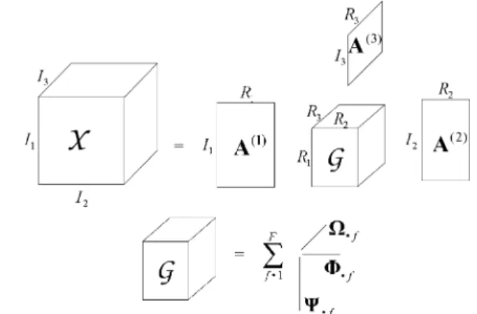
Relation With the Tucker3 Decomposition: It is worth noting that (9) takes the form of a constrained Tucker3 decomposi-tion [11], [13], [14] with the particular characteristic of having a PARAFAC-decomposed core tensor. The main difference be-tween CONFAC and Tucker3 decompositions is in the following aspect. In the Tucker3 decomposition, all the possible factor combinations exist for composing the tensor , where each entry of the Tucker3 core tensor defines the “strength” of each factor combination. Differently, in the CONFAC de-composition, only effectivecombinations take place for com-posing the tensor . In this case, the -factor PARAFAC de-composition of the constrained core tensor reveals the pat-tern of combinations involving the columns of the factor ma-trices , and . Fig. 1 provides an illustration of the CONFAC decomposition.
Relation With the PARAFAC Decomposition: Let us consider
the CONFAC decomposition (3) with and
Fig. 1. Visualization of the CONFAC decomposition of a third-order tensor.
. In this case, the CONFAC decomposition coincides with the -factor PARAFAC decomposition [1]
(11)
Matrix Representations: The CONFAC decomposition can be represented in matrix forms. Two different matrix
represen-tations of the tensor are possible, namely the
slicedandunfoldedrepresentations. Their construction is sim-ilar to that of the standard PARAFAC decomposition [1], [17].
Let us define as a matrix obtained by slicing
the tensor along its first dimension. Similarly,
and are matrices obtained
by slicing the tensor along its second and third dimensions, re-spectively. These matrix-slices can be expressed as a function
of and , by the following set of
equations:
(12)
(13)
(14)
The full information contained in the tensor can be organized in threeunfolded matrices
, and . These matrices are constructed
from the sets of matrix-slices
..
. ... ...
, and can be expressed by the following set of equations:
(15)
(16)
Proof: The proof of (12) and (17) is simple. It is similar to the one presented in [29] for the PARAFAC and Tucker decom-positions. The CONFAC decomposition (3) can be rewritten as
(18)
which means that
..
. ...
and
.. .
.. .
Using (1), we straightforwardly obtain
The factorization of and can be demonstrated in a similar way.
Relation With the PARALIND Model: By comparing (18) with the standard PARAFAC decomposition (11), we remark that the CONFAC decomposition can be viewed as an -factor PARAFAC decomposition with equivalent (rank-deficient) matrices
. The rank-deficient struc-ture due to the repetition of some columns of and , is controlled by the constraint matrices and , respectively. A rank deficient tensor model using constraint matrices is proposed in [16]. This tensor model, which is called PARALIND, makes use of two constraint matrices to model interaction patterns between columns of different factor matrices. In the PARALIND model, the number of factor com-binations/interactions is equal to the number of columns of the factor matrix that is not rank-deficient. The PARALIND model can be obtained from the CONFAC one by making and . Therefore, the CONFAC tensor model can be viewed as a generalization of the PARALIND one.
Interpretation as a Constrained Tucker3 Decomposition:
As aforementioned, the CONFAC decomposition can be interpreted as a constrained Tucker3 decomposition with PARAFAC-decomposed core tensor. We can rewrite (15)–(17)
as a function of the constrained core tensor .
Let us define and
as slices of the constrained core tensor along its first, second and third dimensions, respectively. In order to factorize the unfolded matrices as a function of
the constrained core tensor , we apply the
property (2) yielding the following expressions:
(19)
(20)
(21)
where
(22) (23) (24)
are the three unfolded representations of the constrained core tensor , with
Taking the property (1) into account, we have
..
. ... (25)
where
(26)
In the same way, we get
(27) (28)
Definition 1 (Interaction Matrices): Theinteraction matrices
of the CONFAC decomposition (3) characterize the interaction pattern involving the factors of different pairs of modes. They are defined by
(29)
(30)
where we have used property (5). Similarly, we define
and . Using (8),
the three interaction matrices satisfy the following relation:
(32)
where and are the entries of
and , respectively. We can distinguish the two following situations:
• means that there is no interaction between the
th column of and the th column of , with
or ;
• means that there are interactions
between the th column of and the th column of .
Example 1: Let us consider the CONFAC decomposition of a third-order tensor with
characterized by the following constraint matrices:
(33)
From (29)–(31) we have
indicates that and interact twice. The same
is valid for and . From , we can see that
interacts with while interacts with
. According to , there is an interaction
between and while interacts with
, and with . Summing the nonzero elements
of and yields the number of factor
combinations.
Example 2: Now, consider ,
with constraint matrices having the following structure:
(34)
yielding the following interaction matrices:
According to , each column of interacts with a dif-ferent column of . In particular, interacts twice with . We also have interacting once with and twice
with as indicated by . On the other hand,
in-teracts twice with and once with .
III. UNIQUENESS
The uniqueness of the factor matrices of
the CONFAC decomposition (up to permutation and scaling) depends on the particular structure of the constraint matrices . Specifically, the degrees of freedom introduced in the decomposition by the three constraint matrices can induce a transformational ambiguity over (at least a subset of) the columns of the factor matrices.
Theorem 1 (Identifiability): Let us consider the CONFAC decomposition (3) of a third-order tensor with factor
combinations. Suppose that and are full
column-rank, and that the joint structure of is such
that , and
are also full column-rank, then the decomposition is identifiable in the least squares (LS) sense from (19)–(21).
Proof: Recall the following properties. For
and , with full column-rank,
we have
(35) (36)
Let us define the following quantities:
Identifiability of , in the LS sense, from
(19)–(21) requires that be full column-rank
to be left-invertible. Since , are full
column-rank, using (35) implies that ,
are also full column-rank. From (36), we conclude that since is assumed to be full column-rank, and, thus, is itself full column-rank. The reasoning is similar for .
Identifiability of and in the LS sense means
that they are unique up to a multiplication by a nonsingular
matrix, i.e., any alternative set yielding the
same tensor is linked to the true set by
with and
satisfying the following equality:
(37)
Definition 2 (Admissible Transformation Matrices): The
transformation matrices and are called
admis-sibleif and only if they preserve the constrained structure of the decomposition, which means that (37) is satisfied.
Definition 3 (Essential Uniqueness) [6]: Essential
unique-ness means that any alternative set giving
up to permutation and scaling of their columns, implying admis-sible transformation matrices of the form
(38)
where are diagonal matrices satisfying the relation , and are permutation matrices. A proof of (38) is given in [10] for the PARAFAC decomposition, which also applies here using a similar reasoning.
Definition 4 (Partial Uniqueness): The CONFAC de-composition is said to be partially unique (or restrictively nonunique), when a subset of the columns belonging to the set are essentially unique while the remaining columns are affected by a linear transformation. Partial unique-ness was first observed in [5], and also investigated in [18] and [30] in the context of the standard PARAFAC decomposi-tion. For the CONFAC decomposition, the partial uniqueness property is linked to the structure of the interaction matrices. It can also be studied from equivalence relations between pairs of constraint matrices. We now present sufficient (but not necessary) conditions for partial uniqueness of the CONFAC decomposition implying essential uniqueness in one or two modes.
Theorem 2 (Partial Uniqueness): Consider the CONFAC
de-composition of in terms of factor matrices
and , and characterized by interaction matrices and . Suppose that the three factor matrices contain no zeros. We have the following.
C.1) If , then is
essentially unique.
C.2) If , then is
essentially unique.
C.3) If , then is
essentially unique. Note that
only happens when
. For instance, when
, only is guaranteed to be essen-tially unique, while and are not guaranteed to be unique since only condition 1 of Theorem 2 is satisfied. In this case, however, partial uniqueness (i.e., essential uniqueness of a subset of columns) of and is possible. The degree of partial uniqueness depends on the joint interaction structure of the decomposition. The only case where all the three above conditions are simultaneously satisfied is the one
with , in which the CONFAC decomposition
is close to the PARAFAC one. If and/or
, the essential uniqueness of is not guaranteed by Theorem 2. It should be noted that the three above conditions are sufficient but not necessary for the essential uniqueness of the factor matrices of the decomposition.
Definition 5 (Equivalent Constraint Matrices): When
(respectively, or ), the matrix set
(respectively, or ) is said to beequivalentif
(39)
where are arbitrary permutation matrices.
Note that the equivalence of two constraint matrices means that they are identical up to permutation of their rows. For in-stance, the equivalence between and implies that
and have the same column repetition pattern (up to permutation of the columns of ). Consequently, the matrix-slice factorization defined in (14) can be rewritten as
(40)
where is a diagonal matrix. Note
that (40) is similar to a PARAFAC factorization of the matrix-slice up to permutation and scaling. Similarly, when
or , we have, respectively
(41)
(42)
Therefore, the essential uniqueness of in (40), or
or in (41)–(42) follows from that of
the PARAFAC decomposition.
Partial Uniqueness Corollaries: Using Theorem 2 and the concept of equivalence between constraint matrices given by (39), we can deduce the following partial uniqueness corollaries.
C.1) When and is an equivalent set,
we have
• essentially unique;
C.2) When and is an equivalent set,
we have
• essentially unique;
C.3) When and is an equivalent set,
we have
• essentially unique.
From these corollaries, the essential uniqueness in two modes comes at the expense of a restrictive nonuniqueness in the re-maining mode. Such a “uniqueness tradeoff” is inherent to the CONFAC decomposition. For an illustrative purpose, we can apply corollary C.1 to Example 1 for concluding that and
are essentially unique while is nonunique.
IV. SPACE-TIMESPREADINGMIMO SYSTEM
Inspired on the CONFAC decomposition, we present a new MIMO transmission system. We consider a point-to-point MIMO system with transmit antennas and receive an-tennas. At the transmitter, input data streams are transmitted using spreading codes and transmit antennas. The pro-posed transmission model consists in: i) generating output signals to be transmitted by spreading input data streams2
with the aid of spreading codes and then ii) associating these output signals with the transmit antennas. The simulta-neous transmission of the data streams across multiple transmit antennas may use different codes, or fully reuse the same code, or partially reuse one, or a set of, spreading code(s). Such a
2TheRinput data streams can be assumed to be associated withRusers in
code reuse pattern will be explicitly modeled by exploiting the CONFAC structure, as will be clarified in Section IV-A.
Let denote the spreading factor of the system, i.e., each
symbol is composed of chips of duration
sec-onds, where is the symbol period. We assume that is known or has been estimated (e.g., using cyclostationarity tests). Each input data stream is a packet of symbols. Let
denote the th symbol of the th data stream, the th chip of the th symbol periodic spreading code and the spatial channel gain between the th transmit antenna and the th receive antenna. Each transmit-receive antenna pair is assumed to be characterized by an independent Rayleigh flat fading. Let us define the following matrices
as thesymbol,code,channel matrices, where
are the respective entries of these matrices. We assume that the propagation channel between each pair of transmit and receive antennas is characterized by a finite number of resolvable mul-tipaths. The multipath channel is assumed to be constant during symbols. We assume small angle-spread around the receiver, which arises when the multipath reflectors are in the far field of the receive antenna array [31]. Intersymbol interference (ISI) is handled by assuming that the codes include trailing zeros, or “guard chips” (further details are given in [17]). In this case, only interchip interference (ICI) exists, and the known codes are transformed intounknown“effective signature codes,” given by the convolution of the transmitted spreading codes with the impulse response of the multipath channel, with denoting the number of ISI-free chips per symbol. Under the assumption of independent multipath propagation, the effective signature codes (henceforth referred to as “spreading codes”) are pseu-dorandom and mutually independent codes.
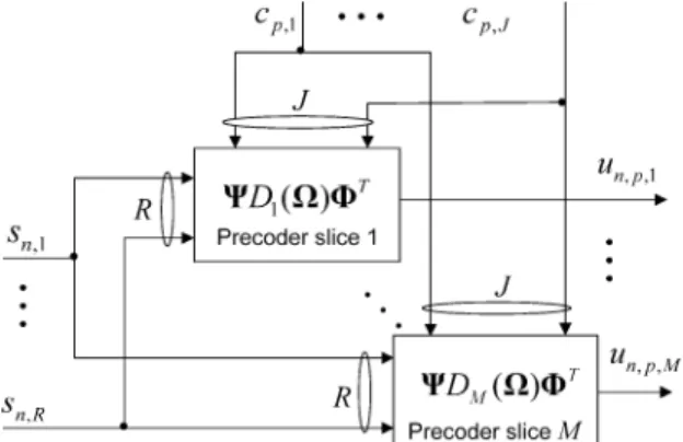
A. Precoder Decomposition
The signal to be transmitted is modeled as the sum of pre-codedsignal components. Let be the th element of theprecoder tensor . This tensor determines the allocation of the th data stream and the th spreading code to the th transmit antenna. The -factor decomposition of the precoder tensor is given, in scalar form, by the following “con-strained” PARAFAC decomposition:
(43)
arestream allocation,
code allocationandantenna allocationmatrices, respectively. Therefore, the precoder tensor can be viewed as ajoint stream-code-antenna multiplexerwhich is decomposed in terms of elementary stream, code and antenna allocation
ma-trices. For instance, means that the th data
stream of the th precoded signal is spread by the th spreading code and then transmitted by the th transmit antenna.
B. Transmitted Signal Model
The precoded signal tensor is represented by the third-order
tensor with entry . The discrete-time
baseband version of the precoded signal associated with the th transmit antenna, th symbol and th chip, is defined
as . We propose the following
constrained factorization for modeling the effective transmitted signal:
(44)
By comparing (44) with (9), we deduce the following correspon-dences:
Hence, the transmitted signal model is a special case of the CONFAC decomposition, where the third-mode matrix is equal to the identity matrix.
We can rewrite (44) in the following form:
(45)
is the matrix of stream/code allocation to the th
transmit antenna and means that
the th transmit antenna transmits the th data stream using the th spreading code. The precoded signal slice
associated with the th transmit antenna can be expressed as
(46)
or, equivalently, in terms of the constraint matrices
(47)
The block diagram of the proposed MIMO transmission system is shown in Fig. 2. In this figure, the precoder tensor is shown in terms of its matrix-slices. The th precoder slice generates a tensor signal component at the th transmit antenna by combining transmitted symbols and spreading codes, the
com-bination pattern being determined by and .
Fig. 2. Block-diagram of the proposed MIMO transmission system.
precoded signals are generated using the following con-straint matrices:
We have
(48)
resulting in the following precoded signal slices:
The first data stream is reused at the first and third transmit antennas with two different spreading codes, while the second data stream is transmitted by a single antenna using a single spreading code.
Example 4: Now, let us consider that we have
and , with the following precoder constraint matrices:
We have
(49)
From (46), we deduce that
In this case, the first and second data streams are code-multi-plexed at the first transmit antenna. The first and second data streams are also, respectively, allocated to the second and third transmit antennas in order to achieve transmit spatial diversity. Several transmit schemes can be designed for a fixed param-eter set , by varying the pattern of 1’s and 0’s of the precoder constraint matrices.
C. Received Signal Model
The discrete-time complex baseband received signal at the th symbol period, th chip and th receive antenna is defined
as being the th
element of thereceived signal tensor collecting the received samples associated with symbols, chips and receive antennas. Using (44), can be written, in absence of noise, as
(50)
which is a CONFAC decomposition of the received signal, with the symbol, code and channel matrices as factor matrices, and with the constrained structure determined by the precoder
tensor . The following correspondences can be
deduced by comparing (9) with (50):
(51)
Let be the slice of the received signal tensor associated
with the th receive antenna, . Using (51) and
(14), we get
We also have
The unfolded matrices and
V. BLINDSYMBOL/CODE/CHANNELRECOVERY
The final goal of our MIMO transmission system is the blind recovery of the transmitted data without using training sequences and without needing a priori explicit channel knowledge or estimation. As discussed in Section III, the partial uniqueness property of the CONFAC decomposition leads to a sort of “uniqueness tradeoff,” where the essential uniqueness in one (or two) mode(s) comes at the expense of a restrictive nonuniqueness in the other mode(s). The implications of such an uniqueness tradeoff in terms of blind symbol/code/channel recovery are now studied. Recall that the uniqueness conditions of Section III estab-lish equivalences between pairs of constraint matrices ensuring essential uniqueness in two factor matrices of the CONFAC decomposition. Having the correspondences (51) in mind, these equivalences admit a physical interpretation in terms of allocation of data streams and spreading codes to transmit antennas, leading to different blind symbol/code/channel recovery properties. We shall distinguish the precoder strategies in two groups: those with reuse in two dimensions only, and those allowing reuse in all the dimensions. These two cases are considered here.
1) Case 1: Reuse in Two Dimensions Only: We assume that either i) data streams and spreading codes are reused more than once in generating the precoded signals, or ii) transmit an-tennas and data streams are reused more than once. These two configurations are detailed here.
1.a) (no transmit antenna reuse): Each
data stream is associated with a different spreading code. Each data stream/spreading code can be reused more than once by different transmit antennas (spatial diversity).
2.a) (no spreading code reuse): Each
transmit antenna is associated with a different data stream. Each data stream/transmit antenna can be reused more than once by different spreading codes (code diversity).
2) Case 2: Reuse in All the Dimensions: We assume that data streams, spreading codes and transmit antennas are reused more than once in generating the precoded signals. We consider two different situations.
1.b) : Equal number of data streams and
codes.
2.b) : Equal number of data streams and
transmit antennas.
From the partial uniqueness corollaries C.1 [for 1.a) and 1.b)] and C.3 [for 2.a) and 2.b)] given in Section III, we can conclude the following.
• For configurations 1.a) and 1.b), if and are equivalent, then both and are essentially unique, i.e.,joint symbol-coderecovery can be achieved.
• For configurations 2.a) and 2.b), if and are equivalent, then both and are essentially unique, i.e.,joint symbol-channelrecovery can be achieved.
These results illustrate the link between the space-time precoder structure with constraints used at the transmitter and the sulting blind symbol/code/channel recovery property at the re-ceiver using the proposed CONFAC model. Several degrees of freedom for space-time precoder design are available for en-suring the blind symbol recovery.
It is worth noting that for configurations with more transmit antennas than data streams (meaning that there is one or more
data streams spatially spread using multiple transmit antennas), the proposed transmission model is similar to space-time spreading [32]–[34]. On the other hand, if we have more data streams than transmit antennas (meaning that two or more data streams are code-multiplexed at the same transmit antenna), the proposed transmission model is close to space-time multi-plexing [35], [36].
Receiver Algorithm: Alternating Least Squares: The pro-posed blind detection algorithm is based on the well-known Alternating Least Squares (ALS) algorithm [11], [17], which is the classical solution for estimating the factor matrices of a tensor model in an iterative way. In our case, the ALS algorithm consists in fitting a CONFAC model to the received signal tensor represented by means of its unfolded matrices as in (15)–(17) to estimate the symbol, code and channel matrices in presence of an additive white Gaussian noise. Since the precoder constraint matrices and are known at the receiver, they are fixed during the whole iterative estimation process.
Define , as the noisy versions
of , where is an additive complex-valued white Gaussian noise matrix. The algorithm consists of the following steps.
1) Set ;
Randomly initialize and ;
2) ;
3) Using ,find an LS estimate of
4) Using ,find an LS estimate of
5) Using ,find an LS estimate of
6) Repeat steps 2-5 until convergence. The convergence at the th iteration is declared when the error between the received signal tensor and its reconstructed version from the estimated factor matrices does not significantly change between iterations and . The conditional update of each matrix may either improve or maintain but cannot worsen the current fit. It is worth noting, however, that the ALS algorithm is strongly dependent on the initialization, and convergence to the global minimum can be slow. Specifically, the convergence of this algorithm can sometimes fall in regions of “swamps” during which the convergence speed is very small and the error between two consecutive iterations does not significantly decrease [11]. A more efficient initialization strategy consists in first ob-taining an estimation of the column space of and using successive singular value decompositions of
and , respectively. Note that
, and can be factored as in (19)–(21) by taking the correspondences (51) into account. The estimated matrices are linked to the true ones by nonsingular nonadmissible transfor-mation matrices. They can, however, be used as a starting point of the ALS algorithm.
ma-trix generally accelerates the convergence of the ALS algorithm, even with small blocks of received samples [25]. Therefore, ex-ploiting the knowledge of the spreading code matrix (whenever it is available) is beneficial from this viewpoint.
VI. SIMULATIONRESULTS
We present some simulation results for illustrating the performance of the proposed MIMO antenna system based on CONFAC modeling. The ALS algorithm described in the previous section is used for this purpose. We are interested in the symbol and channel recovery with the knowledge or not of the spreading codes at the receiver. The symbol recovery performance is evaluated in terms of the BER averaged over 100 Monte Carlo runs. At each run, the additive noise power is generated according to the signal-to-noise ratio (SNR) value given by
This SNR measure takes into account the effects of multiple transmit/receive antennas, fading and multipath. The spa-tial channel gains are drawn from an i.i.d. complex-valued Gaussian generator while the transmitted symbols are drawn from a pseudorandom quaternary phase shift keying (QPSK) sequence. The BER curves represent the performance averaged on the transmitted data streams. Unless otherwise stated,
receive antennas and signal samples are
assumed throughout the simulations.
The ALS algorithm is strongly dependent on the initialization in the completely blind case (where and are unknown). Indeed, ill-convergence to stationary points generally occurs for bad initializations. At each run, we consider 10 tentative random initializations and the one that gives the smallest error is chosen as initialization of the ALS algorithm. The best initialization corresponds to the one with the smallest error. The scaling am-biguity affecting the estimate of the symbol matrix is solved by assuming that the first symbol of each data stream is equal to 1. In this case, the scaling factor is eliminated by normalizing each column of the estimated symbol matrix by its first ele-ment. Optionally differential modulation/encoding can be used to eliminate this ambiguity [17]. In the unknown spreading code case, the inherent column permutation ambiguity in is re-solved using a greedy least squares -column matching al-gorithm [17].
A. Performance of Different Precoding Schemes
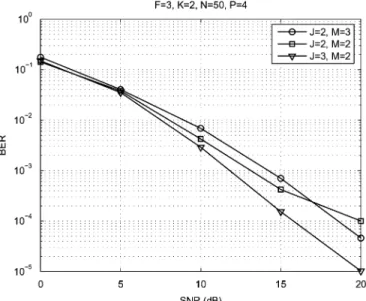
We evaluate the receiver BER performance for some choices of the precoder constraint matrices. We begin by considering a flat-fading channel with the knowledge of the spreading codes at the receiver. We assume precoded signals, or 3 spreading codes, and or 3 transmit antennas. The spreading factor is set to . The orthogonal spreading codes are columns of a Hadamard(4) matrix. The data stream alloca-tion matrix is the one of Example 3 of Section IV-B, which is recalled here for convenience
Fig. 3. Performance of different CONFAC schemes withF = 3.
Three different precoding schemes for 2 or 3 spreading codes/ transmit antennas are tested by varying the structure of the code and antenna allocation matrices and
The BER performance of the three schemes are depicted in Fig. 3. It can be seen that the first and second schemes have similar performance. The third scheme provides the best per-formance due to the fact that the two first schemes reuse one spreading code which is not the case for the third scheme.
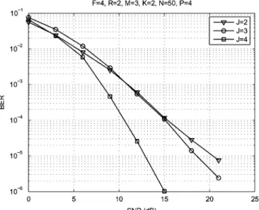
In a second experiment, we assume precoded signals, and , or orthogonal spreading codes. The number of transmit antennas is fixed at , and the spreading factor at . The fixed structure of and is as follows (the same used in Example 4 of Section IV-B):
(52)
According to the structure of and , we can see that each data stream is simultaneously transmitted by two transmit antennas. We consider three code reuse patterns. The three choices for the code allocation matrix are
(53)
Fig. 4. Performance of different CONFAC schemes withF = 4.
different spreading codes. The results are shown in Fig. 4. As ex-pected, the performance improves at the expense of using more orthogonal codes. From the slope of the BER curves, we remark that an increased spatial diversity gain is obtained with the third precoding scheme ( ).
B. Performance With Unknown Spreading Codes
We now consider the case where the spreading codes are un-known at the receiver resulting from the presence of ICI due to multipath/delay propagation. We assume that the channel has chip-spaced multipath components. The multipaths un-dergo independent Rayleigh fading. At each run, the multipath gains are drawn from an i.i.d. complex-valued Gaussian gener-ator. In order to avoid ISI, trailing zeros (guard chips) are included in each spreading code, as discussed in Section IV. We consider two transmit schemes with . The first one
with and ISI-free chips (Hadamard(2) codes
increased by trailing zeros) and the second one with and ISI-free chips. Both schemes have the same antenna reuse pattern and the chosen is the one given in (52). The two other precoding constraint matrices are given below for the first and second schemes, respectively
(54)
(55)
Note that both schemes trade off spatial multiplexing and transmit diversity. In the first one, each data stream is trans-mitted by two transmit antennas. In the second one, spatial multiplexing takes place within the first and second antennas. Both schemes have the same spectral efficiency (the ratio is constant). According to Fig. 5, the first scheme outperforms the second one. This is due to the improved signal separa-tion/resolution that is obtained at the receiver when fewer data streams are transmitted.
Fig. 5. Performance of two transmit schemes with multipath/delay propagation and unknown spreading codes, forR = 2and3.
Fig. 6. CONFAC schemes versus PARAFAC scheme forM = 4.
C. Comparison With a Parafac Scheme
Now, we consider three transmit schemes with
(i.e., ) and . In the first scheme, and are
given by (54). In the second one, we have
The third scheme coincides with the PARAFAC scheme of [17],
where and (no
Fig. 7. Blind CONFAC-ALS versus nonblind CONFAC-ZF receivers.
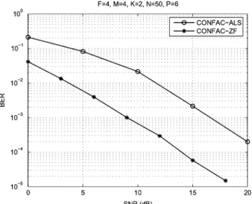
D. Comparison With the Nonblind ZF Receiver
In order to provide a performance reference of the proposed blind receiver (CONFAC-ALS), we have plotted the perfor-mance of the nonblind Zero Forcing (ZF) receiver. Contrarily to the proposed receiver, the nonblind ZF one assumes perfect knowledge of the channel parameters (fading gains and multi-path/delay response) as well as the knowledge of the spreading codes. We consider a frequency-selective channel with multipaths. The spreading codes are unknown at the receiver and . The results are depicted in Fig. 7. The chosen and are given by (54) and . We can observe a gap of, approximately, 7 dB in terms of SNR between blind ALS and
nonblind ZF receivers for .
E. Blind Channel Recovery
As aforementioned, joint blind symbol and channel recovery is possible for some precoder structures with antenna reuse. We evaluate the accuracy of the blind channel estimation from the root mean square error (RMSE) measure averaged over 100 Monte Carlo runs and defined as follows:
where is the channel matrix estimated at the th run. We
consider two schemes with and . Orthogonal
and known spreading codes are assumed with . The struc-ture of these matrices for the first and second schemes are as follows:
Fig. 8 displays the results. The dashed lines are for
and the solid lines for . The results are shown
Fig. 8. RMSE performance for the blind channel estimation.
Fig. 9. Convergence histogram for CONFAC and PARAFAC for 100 runs.
for and receive antennas. In all the simulated config-urations, a linear decrease in the channel estimation error as a function of the SNR is observed. The RMSE increases as the number of data streams/transmit antennas is increased. On the other hand, the estimation accuracy is improved as the number of receive antennas is increased.
F. Evaluation of the Convergence
Fig. 9 depicts an ALS convergence histogram (for 100 Monte Carlo runs) for two transmit schemes: i) CONFAC
scheme with ; ii) PARAFAC scheme
with . For the CONFAC scheme,
constraint matrices. Consequently, the number of parameters to be estimated is smaller with the CONFAC scheme as compared to the PARAFAC one.
VII. CONCLUSION ANDPERSPECTIVES
In this paper, we have presented a new constrained factor decomposition of a third-order tensor, the so-called CONFAC decomposition which consists in a “constrained triple sum” of rank-one third-order tensors, where interactions involving the factors of the decomposition are allowed. The interaction pat-tern is controlled by threeconstraint matrices, each one being associated with one dimension, or mode, of the tensor. The uniqueness tradeoffs of the CONFAC decomposition have been studied and conditions for partial uniqueness, which ensure es-sential uniqueness in one or two modes, have been presented. We have used the CONFAC decomposition to design space-time spreading schemes for MIMO antenna systems with a mean-ingful physical interpretation of the constrained structure of this decomposition. A space-time precoder model fully exploiting the constrained structure of this new decomposition has been presented. We have shown that the CONFAC constraint matrices define the allocation of the data streams and spreading codes to transmit antennas. Based on the CONFAC modeling of the received signal, we have discussed blind symbol/code/channel recovery from the partial uniqueness properties of this decom-position.
Perspectives of this work are multifold. In the area of chemometrics, we expect that the CONFAC decomposition can be exploited to model mixtures of chemical processes with more complicated interaction structures not covered by the PARALIND model [16]. The study of necessary and sufficient conditions in the general case is a topic for future work.
Another perspective concerns the development of efficient algorithms for fitting the CONFAC model, specially in cases where the number of factor combinations is large, or when the constraint matrices of the decomposition are unknown.
With respect to the proposed MIMO antenna system, we must note that the design of the precoder constraint matrices has only focused on uniqueness aspects and has not considered per-formance optimization at the receiver. Several multiple-antenna transmit schemes can be derived by appropriately choosing the structure of these constraint matrices. For fixed precoder param-eters , there exists a finite-set of feasible constraint matrices ensuring blind symbol/channel/code re-covery. We conjecture that limited feedback precoding methods such as those of [37] and [38] can be exploited for selecting the best set of precoder constraint matrices using the estimated MIMO channel. The optimization of the proposed precoder structure from these methods is an interesting research topic to be addressed in a future work.
REFERENCES
[1] R. A. Harshman, “Foundations of the PARAFAC procedure: Model and conditions for an “explanatory” multi-mode factor analysis,”UCLA Working Papers in Phonetics, vol. 16, pp. 1–84, Dec. 1970. [2] J. D. Carroll and J. Chang, “Analysis of individual differences in
mul-tidimensional scaling via an N-way generalization of “Eckart-Young” decomposition,”Psychometrika, vol. 35, no. 3, pp. 283–319, 1970. [3] L. R. Tucker, “Some mathematical notes on three-mode factor
anal-ysis,”Psychometrika, vol. 31, pp. 279–311, 1966.
[4] P. M. Kroonenberg and J. De Leeuw, “Principal component analysis of three-mode data by means of alternating least squares,”Psychometrika, vol. 45, pp. 69–97, 1980.
[5] R. A. Harshman, “Determination and proof of minimum uniqueness conditions for PARAFAC-1,”UCLA Working Papers in Phonetics, no. 22, pp. 111–117, 1972.
[6] J. B. Kruskal, “Three-way arrays: Rank and uniqueness of trilinear de-compositions, with applications to arithmetic complexity and statis-tics,”Linear Algebra Applicat., vol. 18, pp. 95–138, 1977.
[7] J. M. F. ten Berge and N. D. Sidiropoulos, “On uniqueness in CANDE-COMP/PARAFAC,”Psychometrika, vol. 67, pp. 399–409, 2002. [8] T. Jiang and N. D. Sidiropoulos, “Kruskal’s permutation lemma and the
identification of CANDECOMP/PARAFAC and bilinear models with constant modulus constraints,”IEEE Trans. Signal Process., vol. 52, no. 9, pp. 2625–2636, Sep. 2004.
[9] L. De Lathauwer, “A link between the canonical decomposition in mul-tilinear algebra and simultaneous matrix diagonalization,”SIAM J. Ma-trix Anal. Appl, vol. 28, no. 3, pp. 642–666, 2006.
[10] A. Stegeman and N. D. Sidiropoulos, “On Kruskal’s uniqueness con-dition for the Candecomp/Parafac decomposition,”Linear Algebra Ap-plicat., vol. 420, pp. 540–552, 2007.
[11] R. Bro, “Multi-way analysis in the food industry: models, algorithms and applications,” Ph.D. dissertation, Univ. Amsterdam, Amsterdam, The Netherlands, 1998.
[12] H. A. Kiers, J. M. F. ten Berge, and R. Rocci, “Uniqueness of three-mode factor three-models with sparse cores: The 32323 case,” Psychome-trika, vol. 62, no. 3, pp. 349–374, 1997.
[13] H. A. Kiers and A. K. Smilde, “Constrained three-mode factor analysis as a tool for parameter estimation with second-order instrumental data,”
J. Chemomet., vol. 12, no. 2, pp. 125–147, Dec. 1998.
[14] J. M. F. ten Berge and A. K. Smilde, “Non-triviality and identification of a constrained Tucker3 analysis,”J. Chemomet., vol. 16, pp. 609–612, 2002.
[15] J. M. F. ten Berge, “Simplicity and typical rank of three-way ar-rays, with applications to Tucker3 analysis with simple cores,”J. Chemomet., vol. 18, pp. 17–21, 2004.
[16] R. Bro, R. A. Harshman, and N. D. Sidiropoulos, Modeling multi-way data with linearly dependent loadings Univ. of Denmark, Denmark, KVL Tech. Rep. 176, 2005.
[17] N. D. Sidiropoulos, G. B. Giannakis, and R. Bro, “Blind PARAFAC receivers for DS-CDMA systems,”IEEE Trans. Signal Process., vol. 48, no. 3, pp. 810–822, Mar. 2000.
[18] N. D. Sidiropoulos and G. Z. Dimic, “Blind multiuser detection in WCDMA systems with large delay spread,”IEEE Signal Process. Lett., vol. 8, no. 3, pp. 87–89, Mar. 2001.
[19] A. de Baynast and L. De Lathauwer, “Detection autodidacte pour des systemes a acces multiple basee sur 1’analyse PARAFAC,” presented at the 19th GRETSI Symp. Signal Image Process., Paris, France, Sep. 2003.
[20] A. L. F. de Almeida, G. Favier, and J. C. M. Mota, “PARAFAC models for wireless communication systems,” presented at the Int. Conf. Phys. Signal Image Process. (PSIP), Toulouse, France, Jan. 31–Feb. 2 2005. [21] D. Nion and L. De Lathauwer, “A block factor analysis based receiver for blind multi-user access in wireless communications,” presented at the ICASSP, Toulouse, France, May 2006.
[22] L. De Lathauwer and J. Castaing, “Tensor-based techniques for the blind separation of DS-CDMA signals,”Signal Process., vol. 87, no. 2, pp. 322–336, 2007.
[23] A. L. F. de Almeida, G. Favier, and J. C. M. Mota, “PARAFAC-based unified tensor modeling for wireless communication systems with ap-plication to blind multiuser equalization,”Elsevier Signal Process., vol. 87, no. 2, pp. 337–351, Feb. 2007.
[24] L. De Lathauwer, “The decomposition of a tensor in a sum of rank-(Rl,R2,R3) terms,” presented at the Workshop on Tensor Decomposit. Applicat., Marseille, France, 2005.
[25] N. D. Sidiropoulos and R. Budampati, “Khatri-Rao space-time codes,”
IEEE Trans. Signal Process., vol. 50, no. 10, pp. 2377–2388, Oct. 2002. [26] A. de Baynast, L. De Lathauwer, and B. Aazhang, “Blind PARAFAC receivers for multiple access-multiple antenna systems,” presented at the VTC Fall, Orlando, FL, Oct. 2003.
[27] A. L. F. de Almeida, G. Favier, and J. C. M. Mota, “Space-time multi-plexing codes: A tensor modeling approach,” presented at the IEEE Int. Workshop on Signal Process. Adv. in Wireless Commun. (SPAWC), Cannes, France, Jul. 2006.
[29] G. Favier, Calcul matriciel et tensoriel avec applications a 1’automa-tique et au traitement du signal 2008, under preparation.
[30] J. M. F. ten Berge, “Partial uniqueness in CANDECOMP/PARAFAC,”
J. Chemomet., vol. 18, no. 1, pp. 12–16, 2004.
[31] A.-J. van der Veen, “Algebraic methods for deterministic blind beam-forming,”Proc. IEEE, vol. 86, no. 10, pp. 1987–2008, Oct. 1998. [32] B. K. Ng and E. Sousa, “Space-time spreading multilayered CDMA
system,” inProc. IEEE GLOBECOM, Dec. 2000, vol. 3, no. 27, pp. 1854–1858.
[33] B. Hochwald, T. L. Marzetta, and C. B. Papadias, “A transmitter diversity scheme for wideband CDMA systems based on space-time spreading,”IEEE J. Sel. Areas Commun., vol. 19, no. 1, pp. 48–60, 2001. [34] R. Doostnejad, T. J. Lim, and E. Sousa, “Space-time spreading codes for a multiuser MIMO system,” inProc. 36th Asilomar Conf. Signals, Syst. Camp., Pacific Grove, CA, Nov. 2002, pp. 1374–1378. [35] S. Mudulodu and A. J. Paulraj, “A simple multiplexing scheme
for MIMO systems using multiple spreading codes,” inProc. 34th Asilomar Conf. on Signals, Syst. Comp., Pacific Grove, CA, Oct. 2000, pp. 769–774.
[36] R. Doostnejad, T. J. Lim, and E. Sousa, “Space-time multiplexing for MIMO multiuser downlink channels,”IEEE Trans. Wireless Commun., vol. 5, no. 7, pp. 1726–1734, 2006.
[37] R. W. Heath and D. J. Love, “Multimode antenna selection for spa-tial multiplexing systems with linear receivers,”IEEE Trans. Signal Process., vol. 53, no. 8, pp. 3042–3056, Aug. 2005.
[38] D. J. Love and R. W. Heath, “Multimode preceding for MIMO wireless systems,”IEEE Trans. Signal Process., vol. 53, no. 10, pp. 3674–3687, Oct. 2005.
André L. F. de Almeida was born in Teresina, Brazil, in 1978. He received the B.Sc. and M.Sc. degrees in electrical engineering from the Federal University of Ceará, Brazil, in 2001 and 2003, respectively, and the double Ph.D. degree in science and teleinformatics engineering from the University of Nice, Sophia Antipolis, France, and the Federal University of Ceará, Fortaleza, Brazil, in 2007.
He is currently a Postdoctoral Fellow with the I3S Laboratory, Sophia Antipolis. He is also affiliated to the Department of Teleinformatics Engineering of the Federal University of Ceará as an Associated Researcher with the Wireless Telecom Research Group. His research interest lies in the area of signal processing for communications, and include array processing, blind signal separation and equalization, multiple-antenna techniques, and multicarrier and multiuser communications. He has focused on the development of tensor decompositions with applications in MIMO wireless communication systems.
Gérard Favier was born in Avignon, France, in 1949. He received the engineering diplomas from the Ecole Nationale Supérieure de Chronométrie et de Micromécanique (ENSCM), Besançon, France, and Ecole Nationale Supérieure de l’Aéronautique et de l’Espace (ENSAE), Toulouse, France, in 1973 and 1974, respectively. He received the Engineering Doctorate and State Doctorate degrees from the University of Nice, Sophia Antipolis, in 1977 and 1981, respectively.
In 1976, he joined the Centre National de la Recherche Scientifique (CNRS) where he now works as a Research Director of CNRS, I3S Laboratory, Sophia Antipolis. From 1995 to 1999, he was the Director of the I3S Laboratory. His present research interests include nonlinear process modelling and identification, blind equalization, tensor decomposi-tions, and tensor approaches for wireless communication systems.
João Cesar M. Motawas born in Rio de Janeiro, Brazil, in 1954. He received the B.Sc. degree in physics from the Universidade Federal do Ceará (UFC), Brazil, in 1978, the M.Sc. degree from Pontifícia Universidade Católica (PUC-RJ), Brazil, in 1984, and the Ph.D. degree from the Universidade Estadual de Campinas—UNICAMP, Brazil, in 1992, all in telecommunications engineering.
Since August 1979, he has been with the UFC, and currently is Professor with the Teleinformatics Engineering Department. He was with the Institut National des Télécommunications and Institut de Recherche en Communica-tions et Cybernetique de Nantes, both in France, as an Invited Professor during 1996–1998 and spring 2006, respectively. His research interests include digital communications, adaptive filter theory, and signal processing.