1391 1 INTRODUCTION
An application of the finite element method (FEM) for non-linear elastoplastic analysis of rein-forced soil structures under axisymmetric condition is presented in this paper.
The Mohr-Coulomb criterion suggested by Sloan & Booker (1986) and Abbo & Sloan (1995), which includes treatment of the singularities of the original Morh-Coulomb criterion, is used for modeling the foundation soil. A general formulation that considers associative and non-associative elastoplastic models for soil was adopted. Hence, the influence of the dilatancy angle on the bearing capacity of reinforced soil could be investigated. The reinforcement is considered as linear elastic and the soil-reinforcement interface was considered rigid; thus interface ele-ments were not considered in these analyses.
The numerical simulation was conducted using the code ANLOG – Non Linear Analysis of Geotechnical Problems (Zornberg, 1989; Nogueira, 1998; Pereira, 2003; Oliveira, 2006).
2 FINITE ELEMENT REPRESENTATION OF REINFORCED SOIL
A discrete representation for reinforced soil structures is adopted in this study. Each component of reinforced soil structure—the soil, the reinforcement and the soil-reinforcement interface— can be represented using a specific finite element with its own kinematic and constitutive equa-tions. In the specific case of a bearing capacity problem of shallow foundations, the soil-reinforcement interface was considered rigid and therefore is not discussed in this paper.
In considering an incremental formulation by FEM, the kinematic equation that describes the relationship between the increment of strain (ε) and the increment of nodal displacement (uˆ) in each finite element can be written as:
u B
ε ˆ
(1)
FE prediction of bearing capacity over reinforced soil
C.L. Nogueira
Department of Mines Engineering, School of Mine, UFOP, Ouro Preto/MG, Brazil
R.R.V. Oliveira & L.G. Araújo
Department of Civil Engineering, School of Mines, UFOP, Ouro Preto/MG, Brazil
P.O. Faria
Department of Civil Engineering - CTTMar – Univali, Itajaí/SC, Brazil
J.G. Zornberg
Department of Civil Engineering, University of Texas at Austin, Austin/TX, USA
where
N
B (2)
is a differential operator and N is the matrix that contains the interpolation functions Ni. Both
the operator and matrix depend on the type of element adopted. The negative sign in Equation 1 is a conventional indicator of positive compression.
The increment of stress ( ) can be obtained using the incremental constitutive equation:
Dt (3)
where Dt is the constitutive matrix defined in terms of the elastoplasticity formulation as:
p e t D D
D (4)
where De is the elastic matrix and Dp is the plastic parcel of the constitutive matrix defined as:
H ) ( e T T e e p b D a a D b D
D (5)
a is the gradient of the yield function (F(σ,h)), b is the gradient of the potential plastic function (G(σ,h)), h is the hardening parameter and H is the hardening modulus. In the case of perfect plasticity, since hardening is not considered, H equals zero.
Starting from an equilibrium configuration where the displacement field, the strain state, and the stress state are all known, a new equilibrium configuration, in terms of displacements, can be obtained using the modified Newton Raphson procedure with automatic load increment (No-gueira, 1998). In this paper, only the elastic parcel of the constitutive matrix was considered in the iterative procedure used to obtain the global stiffness matrix.
At each increment the iterative scheme satisfies, for a selected tolerance, the global equili-brium, compatibility conditions, boundary conditions and constitutive relationships. Yet atten-tion must be given to the stress integraatten-tion scheme adopted to obtain the stress increments (Equ-ation 3), in order to guarantee the Kuhn-Tucker conditions and the consistency condition. 2.1 Soil representation
The soil is represented by the quadratic quadrilateral isoparametric element (Q8). This element has two degree of freedom, u and v, in the directions r and y (radial and axial), respectively. The stress and strain vectors are defined as:
r y ry
T
σ (6)
r y ry
ε (7)
In which u/r. The kinematic matrix B can be written as:
r N 0 y N 0 y N r N 0 r N r N 0 y N 0 y N r N 0 r N 8 8 8 8 8 1 1 1 1 1
Β (8)
where N
iis the i node shape function by the finite element Q8 (Nogueira, 1998).
Thestiffness matrix for axisymmetric condition for this element is given by:
1 1 1 1 t T d d det ˆ 2( Nr J
B D B
K (9)
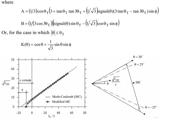
1393 To describe the stress-strain relationship a perfectly elastoplastic model with non-associative plasticity was adopted. The plastic parcel of the constitutive matrix is obtained using the mod-ified Mohr-Coulomb criterion proposed by Sloan & Booker (1986) and Abbo & Sloan (1995) (Figure 1). The modified version of the Mohr-Coulomb model involves removal of the singu-larities at the edges ( 6) and the apex of the original model. Its yield function is written as:
I K( ) asin I 3sin ccos
F 2D 2 2 1 (10)
where
13sin 1
1.5 3
I3D
I2D 3/2
[/6;/6] (11)
is the Lode angle, I1 is the first invariant of the stress tensor; I2D is the second invariant of the desviator stress tensor, I3D is the third invariant of the desviator stress tensor, c and are the
material cohesion and internal friction angle, respectively. A transition angle (T) was intro-duced to define the K() function on the Equation 10. Sloan & Booker (1986)suggest T value range from 25 to 29. For the case in which T,
) A Bsin3 (
K (12)
where
13cos 3 tan tan3 1 3signal( )(3tan tan3 )sin
A T T T T T (13)
1 3cos3 signal( )sin 1 3 cos sinB T T T (14)
Or, for the case in which T
sin sin
3 1 cos ) (
K (15)
c cotan
a
Modified MC Morh-Coulomb (MC)
3 / I1
D 2
I c
I2D
25
25
30
30
MC
c cotan
a
Modified MC Morh-Coulomb (MC)
3 / I1
D 2
I c
I2D
25
25
30
30
MC
Figure 1 - Mohr-Coulomb yield function (Abbo & Sloan, 1995).
The parcel asin was introduced to prevent the singularity related to the surface apex. For the parameter “a” Abbo & Sloan (1995) recommend 5% of (c cotan). The potential plastic function (G) can be written the same way as the yield function (F) but using the dilatancy angle () instead of the friction angle ().
2.2 Reinforcement representation
The reinforcement is represented by quadratic one-dimensional isoparametric elements (R3) (Oliveira, 2006). The reinforcement thickness is considered in the constitutive equation. This element has one degree of freedom, u', on its own longitudinal direction r'. The longitudinal di-rection is related to the radial didi-rection on the local coordinate system according to the following transformation:
rˆ
rNT (16)
In which N is the matrix that contains the shape functions (Ni) for this element (Oliveira, 2006),
1 1 3 3
T
y r y
r
rˆ is the nodal global coordinate vector, and
sen cos 0 0 0 0 sen cos
T (17)
where cos(dr d) detJ; sen(dy d) detJ; detJ (dr/d)2(dy/d)2 ;
3 1 i i i r d dN d dr
and
3 1 i i i y d dN d dy .
The R3 element has two components of strain and stress: longitudinal (r and r) and cir-cumferential ( and ). The kinematic condition is given by the relation:
u J J u ε ˆ r N r N N det 1 N det 1 ˆ 3 1 3 1 (18)
where uˆ is the vector of the nodal global displacement components (u,v). The constitutive matrix for the reinforcement element is given by:
1 ν ν 1 ν 1 t / J 2 tD (19)
where J is the reinforcement stiffness (kN/m), t is the reinforcement thickness and is the Pois-son ratio.
The reinforcement stiffness matrix under axisymmetric condition is given by:
1 1 t T d det ˆ t 2( Nr J
BT D BT
K (20)
3 BEARING CAPACITY ON UNREINFORCED SOIL
1395
10m
10
1m
10m
10m
B=1m
10m
10
1m
10m
10m
B=1m
a)
1m
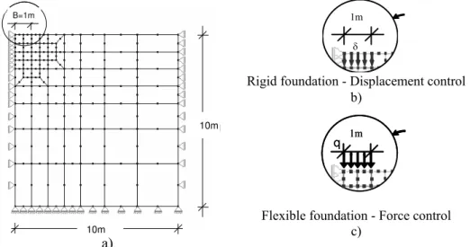
Rigid foundation - Displacement control b)
1m q
1m q
Flexible foundation - Force control c)
E=100Mpa; =0.30; c=10kPa; a=15%; T=29o; and vary
Figure 2 - Finite element mesh: a) full mesh; b) detail of the displacement imposed boundary condition; c) detail of stress imposed boundary condition
An incremental-iterative modified Newton Raphson scheme with automatic loading incre-ments is used considering a tolerance of 10-4 for the force criterion of convergence. For the stress integration algorithm the following tolerances are used: FTOL=10-9 and STOL=10-8. The FTOL tolerance is related to the transition condition from elastic to plastic state which is af-fected by the finite precision arithmetic. The STOL tolerance is related to the local error in the stresses in the Euler modified schemes.
Numerical results are presented in terms of the factor which is a normalized stress defined as:
Ac q/c/
Q
(21)
in which A is the footing area and Q is the reaction force at the foundation, defined as:
n
1
e e e
T
dV Q
e V
σ
B (22)
The reaction force is evaluated as the sum of the internal force’s vertical components equiva-lent to the elements’s stress state right beneath the foundation. The cohesion is adopted to nor-malize the results but in the case of cohesionless soil the atmospheric pressure can be adopted instead.
Figure 3 presents the factor versus normalized settlement (/B) curves obtained by ANLOG for flexible and rigid foundations and for different values of friction and dilatancy angles. It can be observed that associative analysis (=) provides the lowest displacement at failure.
Table 1 presents normalized ultimate bearing capacity (ult), as shown in Figure 3. As
ex-pected, the ult value obtained for rigid foundation is higher than that obtained for a flexible
foundation. The difference in ult values was approximately 9.5%, but the highest difference was
observed in non-associative plasticity (approximately 11.2%).
Analyses conducted in this study show that when the friction angle was decreased to 10° and 20°, the ultimate bearing capacity factor (ult) was no longer affected by the dilatancy angle. For
friction angle of 30° the associate plasticity analysis (=) provided the highest ultimate bearing capacity factor and the lowest displacement at failure. Zienkiewicz et al. (1975) observed a simi-lar response for friction angles of 40°. Monahan & Dasgupta (1993) reported such behavior for friction angles higher than 25°.
(1975), and a recent numerical solution based on limit analyses using FEM by Ribeiro (2005). Good agreement can be observed among these results.
0 0.01 0.02 0.03 0.04 0.05
/B 0
12 24 36 48 60
=10o
=20o
=30o
=30o
=20o ultimate load
0 0.01 0.02 0.03 0.04 0.05
/B
=10o
=30o
=30o
=20o
ultimate load
a) b)
Figure 3 - Load versus displacement curves: a) Flexible foundation; b) Rigid foundation
Table 1 - Normalized ultimate bearing capacity (ultqult/c) ( °) (°) Flexible
Foundation
Rigid Foundation
10 0 10.1 11.4
10 10.4 11.4
20 0 20.0 22.0
20 20.4 22.4
30 0 43.4 49.5
30 49.5 54.0
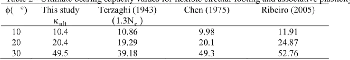
Table 2 - Ultimate bearing capacity values for flexible circular footing and associative plasticity ( °) This study
ult
Terzaghi (1943) (1.3Nc)
Chen (1975) Ribeiro (2005)
10 10.4 10.86 9.98 11.91
20 20.4 19.29 20.1 24.87
30 49.5 39.18 49.3 52.76
4 BEARING CAPACITY ON REINFORCED SOIL
A rigid rough circular shallow foundation subjected to vertical loading is analyzed using differ-ent reinforcemdiffer-ent configurations. The soil is considered frictionless, weightless and elastic per-fectly plastic with the following properties: E=10MPa; =0.49, c=30kPa, =0o, a=0, T=28o. The
1397 0.5m
5m 4.5m
Figure 4 - Finite element mesh – Rigid rough circular without embedment shallow foundation
Figure 5 illustrates the reinforcement layout considered in this study. B is the circular footing diameter, U is the depth to the first reinforcement layer, H is the space between each reinforce-ment layer, N is the number of reinforcereinforce-ment layers; b is the diameter of reinforced zone and d is the depth of the last reinforcement layer.
B
b
U H H
H d
1 2 3
N-1 N
Figure 5 - Layout of the rigid foundation on reinforced soil
4.1 Unreinforced foundation
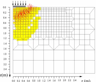
For an unreinforced foundation, the ult value obtained by ANLOG was 5.42. Potts and Zdravković (2001) have obtained 5.39. The difference, approximately 0.5%, is considered neg-ligible. At this level the settlement obtained by ANLOG was 0.025m.
Figure 6 illustrates the failure mechanism with displacement vectors. The failure mechanism is consistent with that proposed by Prandtl (1920) for strip footing.
r (m) z(m)
r (m) z(m)
4.1 Reinforced foundation
Prediction of the bearing capacity was initially conducted considering a single layer of rein-forcement under axisymmetric condition. The diameter of the reinforced zone is constant (b=4B) while the reinforcement depth varies from 0.05 B to 0.9 B.
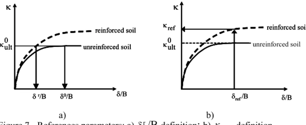
The bearing capacity improvement is evaluated by quantifying the bearing capacity ratio (BCR) defined as:
0 ult
BCR
(23)in terms of the
κ
factor for the reinforced soil foundation and the ultimate bearing capacity for the unreinforced soil foundation (0ult ). For consistency, the BCR must be evaluated at a par-ticular settlement level. For instance, BCR0.1 means the bearing capacity improvement is beingevaluated with the
κ
factor at a normalized settlement (/B) of 0.1.The settlement reduction improvement is evaluated by the settlement reduction ratio (SRR) which is defined as:
%
100
SRR
0r 0
(24)where
0 is the settlement at the ultimate load of unreinforced foundation soil and
r is the set-tlement of reinforced foundation soil at the ultimate load of unreinforced soil foundation. Figure 7 illustrates these indexes.r/B 0/B
reinforced soil unreinforced soil
/B
0 ult
ref/B
reinforced soil unreinforced soil
/B
0 ult
ref
r/B 0/B
reinforced soil unreinforced soil
/B
0 ult
r/B 0/B
reinforced soil unreinforced soil
/B
0 ult
ref/B
reinforced soil unreinforced soil
/B
0 ult
ref
ref/B
reinforced soil unreinforced soil
/B
0 ult
ref
a) b) Figure 7 - References parameters: a) r
/B
definition;
b)ref
definition
As expected, the settlement decreases because of the reinforcement of the foundation soil. A region can be defined through where the reinforcement location maximizes the SRR. In this case the higher value of SRR was around 40% from 0.05B to 0.35B (Figure 8). In terms of bearing capacity improvement, the results provided in Figure 8 indicate that there is little improvement for a single layer of reinforcement (maximum BCR was 14%). It should also be noted that there is an optimum depth as well as a limit depth, beyond which no improvement is verified.
Figure 9 presents the displacement field at the failure for unreinforced soil foundation and the optimum and limit reinforcement positions. Note that the limit depth (Ulimit) coincides with the
lowest point of the failure wedge and the optimum depth (Uoptimum) coincides with a high level of
mobilized shear stress for the unreinforced foundation soil.
1399
0 0.2 0.4 0.6 0.8 1
U/B 1
1.04 1.08 1.12 1.16
BC
R
(ref=0.1 B
reinforcement U
0 0.2 0.4 0.6 0.8 1
U/B 10
20 30 40 50 60
SR
R
(
%
)
B
reinforcementU
(ref=0.1
Figure 8 - U/B influence on the BCR and the SRR
Uoptimum Ulimit
Uoptimum Ulimit
Figure 9 - Optimum and limit reinforcement position
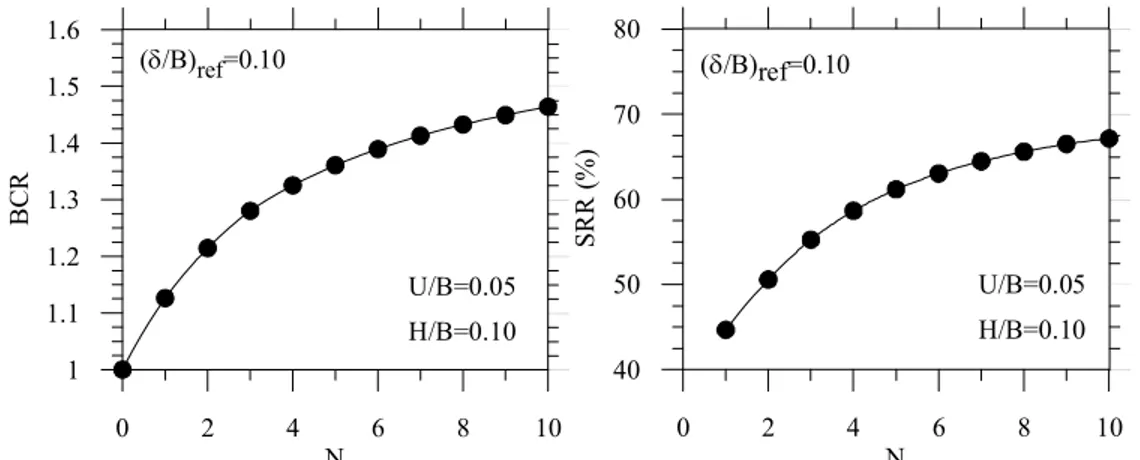
0 2 4 6 8 10
N 1
1.1 1.2 1.3 1.4 1.5 1.6
BC
R
(/B)ref=0.10
U/B=0.05
H/B=0.10
0 2 4 6 8 10
N 40
50 60 70 80
SRR (
%
)
(/B)ref=0.10
U/B=0.05
H/B=0.10
Figure 10 - Influence of the number of reinforcement layers
In this case, which involved circular footing and frictionless soil foundation, the bearing ca-pacity improvement (BCR) was around 10% and the settlement reduction ratio (SRR) was around 6% as the number of reinforcements was increased from 5 to 10. Accordingly, the num-ber of reinforcement layers should not exceed 4 to 7.
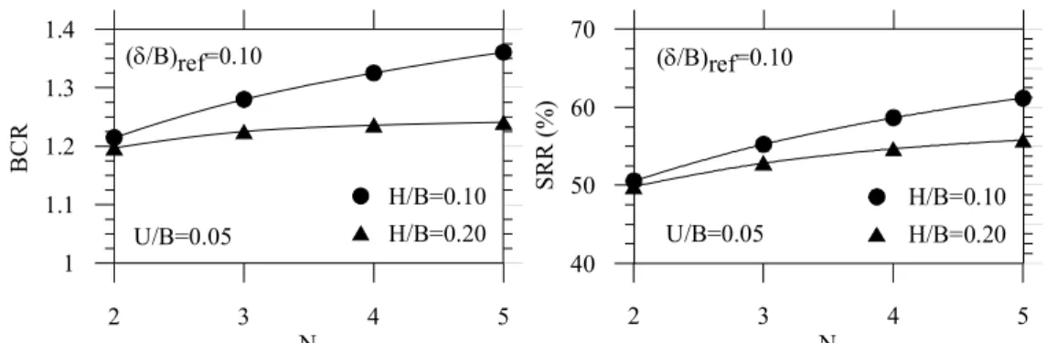
2 3 4 5 N
1 1.1 1.2 1.3 1.4
BC
R
H/B=0.10
H/B=0.20 (/B)ref=0.10
U/B=0.05
2 3 4 5
N 40
50 60 70
SRR (
%
)
H/B=0.10
H/B=0.20 (/B)ref=0.10
U/B=0.05
Figure 11 - Influence of the space between each reinforcement layer
Figure 12 shows the horizontal displacement field of the unreinforced soil and of two confi-gurations of reinforced soil (H/B=0.10 and H/B=0.20). This displacement field is at the settle-ment level corresponding to an ultimate level of unreinforced soil (/B=0.05). The number of reinforcement layers (N=5) and the position of the first reinforcement layer (U/B=0.05) are con-stant. The lowest horizontal displacement was observed when the H/B is 0.10. As expected, the results confirmed that high confinement improves bearing capacity.
U/B=0.05 H/B=0.20
U/B=0.05 H/B=0.10 U/B=0.05
H/B=0.20
U/B=0.05 H/B=0.10
Figure 12 - Horizontal displacement (m) – rigid foundation (ref/B=0.1)
Adopting the foundation settlement reference (ref) of 0.05 m and maintaining B=1m,
H/B=0.1, N=5 and b/B=4 as constant, the influence of the depth of the first reinforcement layer (U) was analyzed. In order to explain this influence the curve BCR versus U/B (Figure 13) was divided into 3 zones in terms of the bounded values (U/B)optimum and (U/B)limit. Zone 1 defines
the suitable values for the position of the first layer. Zone 2 is characterized by a significant de-crease in the bearing capacity ratio. In Zone 3 shows no improvement in bearing capacity. In this case the bounded values, (U/B)optimum and (U/B)limit, was respectively around 0.05 and 0.25.
0 0.1 0.2 0.3 0.4 0.5 0.6
U/B 1
1.1 1.2 1.3 1.4
BC
R
(U/B)optimum
(U/B)limit
Zone 2 Zone 3
Zo
ne
1
H/B=0.10 N=5
1401 Figure 14 shows the failure mechanisms for the case in which the depth of the top reinforce-ment layer exceeds (U/B)limit. Note that the reinforced layer of soil works as a rigid and rough
base. In this region both vertical and horizontal displacements are approximately zero.
z(m) z(m)
Figure 14 - Influence of the first reinforcement layer depth – (ref/B=0.1)
5 CONCLUSIONS
This paper presented a numerical simulation using FEM to analyze the bearing capacity of shal-low foundations on reinforced soil under axisymmetric conditions. The modified Mohr-Coulomb constitutive model was implemented into ANLOG. The implementation of the explicit integration stress algorithm proposed by Sloan et al (2001) was needed in order to obtain good performance of the Newton Raphson algorithm at the global level.
The numerical results confirmed that the ultimate bearing capacity of a rigid shallow founda-tion on unreinforced soil is higher than that on a flexible shallow foundafounda-tion. The ultimate bear-ing capacity of flexible foundations obtained numerically shows good agreement with the results obtained by equilibrium limit theory (Terzaghi, 1943) and limit analysis (Chen, 1975; Ribeiro, 2005).
The ultimate bearing capacity of unreinforced soil was not affected by the dilatancy angle when the friction angle is low but is relevant for comparatively high friction angles. Therefore, for a high friction angle the ult values are a little high in the case of associative plasticity. In
general, the non-associative plasticity provides higher settlement at failure. Results presented in this paper agree with the results provided by Monahan & Dasgupta (1995) and Zienkiewics et al (1975).
In order to show the influence of the reinforcement on the bearing capacity and settlement re-duction, a parametric study was conducted using different reinforcement configurations. A rigid, rough, and shallow foundation under axisymmetric condition was considered in the analysis. The soil foundation was considered weightless and purely cohesive (=0) and the interface soil-reinforcement was considered rigid. Based on the results, it may be concluded that:
The bearing capacity increases and the settlement reduction increases as the number of rein-forcement layers increase. A cost-benefit analysis should be conducted to define the optimum number of reinforcement layers to be used.
The bearing capacity ratio, which indicates the improvement on the bearing capacity, was ap-proximately 14% for just one reinforcement layer; it may be considered modest. In this case the optimum depth for placing it is 0.1B and the limit depth is 0.5B. The reinforcement influence on the settlement, however, is significant (around 40% to 50%). The reinforcement starts to work after the soil deforms plastically, which often occur at a high level of settlement.
ACKNOWLEDGMENTS
The authors are grateful for the financial supports received by the first author from CAPES (Coordinating Agency for Advanced Training of High-Level Personnel – Brazil) and by the second author from Maccaferri do Brasil LTDA. They also acknowledge the Prof. John Whites for the English revision of this text.
REFERENCES
Abbo, A.J. & Sloan, S.W. 1995. A smooth hyperbolic approximation to the Mohr-Coulomb yield crite-rion. Computers & Structures, 54(3): 427-441.
Chen, W.F. 1975. Limit Analysis and Soil Plasticity. Elsevier Science Publishers, BV, Amsterdam, The Netherlands.
Houlsby, G.T. 1991. How the dilatancy of soils affects their behaviour, Proc. X Euro. Conf. Soil Mech. Found. Engng., Firenze 1991, (4):1189-1202.
Manohan, N. & Dasgupta, S.P. 1995. Bearing capacity of surface footings by finite element. Computers & Structures, (4): 563-586.
Nogueira, C.L. 1998. Non-linear analysis of excavation and fill. DS. Thesis. PUC/Rio, RJ, 265p (in Portu-guese).
Oliveira, R.R.V. 2006. Elastoplastic analysis of reinforced soil structures by FEM. MS. Thesis. PRO-PEC/UFOP (in Portuguese).
Pereira, A.R. 2003. Physical non-linear analysis of reinforced soil structures. MS. Thesis. PROPEC/UFOP (in Portuguese).
Potts. D.M. & Zdravković, L. 2001. Finite Element analysis in geotechnical engineering: application. Thomas Telford Ltda.
Ribeiro, W.N. 2005. Applications of the numerical limit analysis for axisymmetric stability problems in Geotechnical Engeneering. MS. Thesis, UFOP (in Portuguese).
Sloan, S.W. & Booker, J.R. 1986. Removal of singularities in Tresca and Mohr-Coulomb yield criteria,
Comunications in Applied Numerical Methods, (2): 173-179.
Sloan, S.W.; Abbo, A.J. & Sheng, D. 2001. Refined explicit integration of elastoplastic models with automatic error control, Engineering Computations, 18(1): 121-154.
Terzaghi, K. 1943. Theoretical Soil Mechanics. Wiley.
Zienkiewicz, O.C., Humpheson, C. & Lewis, R.W. 1975. Associated and non-associated visco-plasticity and plasticity in soil mechanics. Geotechnique, 25(4): 671-689.