Atmos. Meas. Tech., 8, 4917–4930, 2015 www.atmos-meas-tech.net/8/4917/2015/ doi:10.5194/amt-8-4917-2015
© Author(s) 2015. CC Attribution 3.0 License.
Sensitivity of remotely sensed trace gas concentrations
to polarisation
D. M. O’Brien1, I. N. Polonsky2, and J. B. Kumer3
1Greenhouse Gas Monitor Australia Pty Ltd, Melbourne, Australia 2RT and RS Solutions, Tucson, USA
3Advanced Technology Center, Lockheed-Martin, Palo Alto, USA
Correspondence to:D. M. O’Brien ([email protected])
Received: 5 June 2015 – Published in Atmos. Meas. Tech. Discuss.: 24 August 2015 Revised: 29 October 2015 – Accepted: 29 October 2015 – Published: 23 November 2015
Abstract. Current and proposed space missions estimate column-averaged concentrations of trace gases (CO2, CH4
and CO) from high resolution spectra of reflected sunlight in absorption bands of the gases. The radiance leaving the top of the atmosphere is partially polarised by both reflection at the surface and scattering within the atmosphere. Gener-ally, the polarisation state is unknown and could degrade the accuracy of the concentration measurements. The sensitiv-ity to polarisation is modelled for the proposed geoCARB instrument, which will include neither polarisers nor polari-sation scramblers to select particular polaripolari-sation states from the incident radiation. The radiometric and polarimetric cal-ibrations proposed for geoCARB are outlined, and a model is developed for the polarisation properties of the geoCARB spectrographs. This model depends principally upon the effi-ciencies of the gratings to polarisations parallel and perpen-dicular to the rulings of the gratings. Next, an ensemble of polarised spectra is simulated for geoCARB observing tar-gets in India, China and Australia from geostationary orbit at longitude 110◦E. The spectra are analysed to recover the trace gas concentrations in two modes, the first denied access to the polarimetric calibration and the second with access. The retrieved concentrations using the calibration data are al-most identical to those that would be obtained with polarisa-tion scramblers, while the retrievals without calibrapolarisa-tion data contain outliers that do not meet the accuracies demanded by the mission.
1 Introduction
The Greenhouse gases Observing SATellite (GOSAT) launched by Japan’s Aerospace Exploration Agency esti-mates column-averaged concentrations1 of CO2 and CH4
from high resolution spectra of reflected sunlight in absorp-tion bands of CO2, CH4and O2. Similarly, NASA’s second
Orbiting Carbon Observatory (OCO-2) estimates CO2from
CO2 and O2 spectra. While GOSAT measures two
orthog-onal polarisations, OCO-2 measures only one. In contrast, geoCARB (Sawyer et al., 2013; Mobilia et al., 2013; Kumer et al., 2013; Polonsky et al., 2014; Rayner et al., 2014), pro-posed to measure CO2, CH4 and CO from a geostationary
platform, will have inherent sensitivity to polarisation, prin-cipally through the diffraction gratings, but will not have any hardware (like GOSAT) or adopt any flight manoeuvres (like OCO-2) to select specific polarisations. The question arises as to whether the sensitivity of the instrument to polarisation causes significant error in retrieved gas concentrations.
This paper uses the following methodology to address this issue. First, in Sect. 2 a model is developed for the polar-ising properties of the geoCARB spectrographs. The model depends on parameters characterising the optics and the po-tentially non-linear responses of the detectors; the procedure by which these parameters will be determined during pre-flight calibration of geoCARB is outlined in Sect. 3. A sim-plified model that requires only the absolute efficiencies of the gratings is described in Sect. 4.
1The term concentration is used here in its common English
Next a numerical simulator is flown over a model world to generate an ensemble of polarised spectra that captures much of the variability seen in the real world. For each spectrum in the ensemble, the Stokes vector is computed at the entrance aperture of geoCARB above the atmosphere, and the intensi-ties falling upon the detectors are simulated using the simpli-fied model. For these simulations, described in Sect. 5, geo-CARB is assumed to be at longitude 110◦E and three frames of data are considered. The first is centred on Agra in India (27.18◦N, 78.02◦E), and consists of 1001 pixels observed si-multaneously in the 4 s integration time of geoCARB. The pixels are aligned approximately north–south, and include ocean in the south and the Himalaya in the north. The sec-ond and third frames, similarly consisting of 1001 pixels, are centred on Wuhan in China (30.35◦N, 114.17◦E) and
Al-ice Springs in Australia (23.42◦S, 133.52◦E). In order to
in-clude a variety of illumination and observation geometries, each frame is sampled three times per day, the first 3 hours before solar noon, the second at solar noon, and the third 3 hours after. Four days are simulated close to the solstices and equinoxes.
In Sect. 6 the simulated signals, computed taking into account the polarising properties of the surface, clouds, aerosols and molecules, are passed to the inversion algorithm that estimates the column-averaged concentrations of CO2,
CH4 and CO, respectively denoted XCO2,XCH4 andXCO.
The inversion algorithm is denied access to the polarising properties of the surface and the atmosphere. Instead it as-sumes that the surface is Lambertian and non-polarising, but it generates polarising elements internally as it allocates and distributes clouds and aerosols while attempting to match its prediction of the intensity incident upon the detector with the “true” intensity from the simulator. The source of polarisa-tion within the retrieval algorithm is via scattering by clouds, aerosols and molecules. Statistics of the differences between the retrieved and true concentrations of CO2, CH4and CO
are analysed in Sect. 7.
The polarisation sensitivity of the geoCARB spectrome-ters imposes strong, wavelength dependent signatures upon the spectra, which raises the question as to whether such sig-natures might cause unacceptably large errors in retrieved concentrations of CO2, CH4and CO. Two experiments are
conducted to assess this risk.
In the first, the inversion algorithm is denied access to the polarisation model of the instrument, thereby forcing it to as-sume that the measured signal represents the intensity at the top of the atmosphere. Although there is some degradation of accuracy for the retrieved concentrations of CO2, CH4and
CO, the errors are not as large as might be expected, because the retrieval algorithm tries to attribute the wavelength signa-tures caused by the polarisation sensitivity of the gratings to the wavelength dependence of other geophysical parameters, especially the surface albedo. As the objective of the geo-CARB mission is to measure trace gas concentrations, and
not to measure albedos, the outcome of this experiment is marginally acceptable.
In the second experiment, the radiometric and polarimet-ric responses of geoCARB are assumed to be calibrated be-fore launch, and the results are made available to the re-trieval algorithm. In this case geoCARB returns trace gas concentrations with accuracy equal (on average) to that of a similar instrument equipped with polarisation scramblers. The latter ensure that the intensity reaching the detectors is the same (apart from a scaling factor) as the intensity arriv-ing at the scan mirror. Thus, provided pre-flight calibration characterises both the radiometric and polarimetric responses of geoCARB, polarisation scramblers should not be needed. This is a fortunate result, because scramblers almost certainly would degrade the spatial resolution and increase both the in-strument complexity and cost.
2 Polarisation model
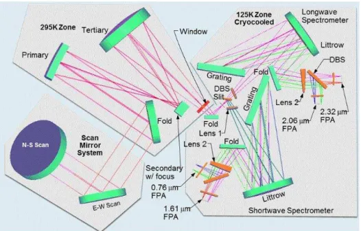
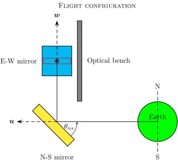
The purpose of the polarisation model is to predict the signal at the detector2from the Stokes vector3of radiation arriving at the entrance aperture of geoCARB. Despite the complexity of the optical layout of geoCARB, shown in Fig. 1, in order to formulate the polarisation model it suffices to divide the op-tics of geoCARB into three logical assemblies, the first two being the moving scan mirrors (north–south and east–west), and the third being the fixed telescope and grating spectro-graph.4The division is shown schematically in Fig. 2, which also indicates the coordinate system used by geoCARB. All quantities in the polarisation model depend on wavelength, but the dependence is not shown explicitly in order to sim-plify the notation.
The transformation of the Stokes vectorS=(I, Q, U, V )T
incident on the north–south scan mirror to the Stokes vector arriving at the detector is described by a Mueller matrix
M=M3M2M1R0. (1)
The factorR0rotates the plane of reference for
polarisa-tion from that used by the radiative transfer model to the re-flection plane of the north–south scan mirror. It has the form
R0=R(η0), (2)
2The signal at the detector is represented by the output
poten-tialv, but equally well could be the output current or the charge
accumulated over an integration period.
3The conventions for polarisation used by Mishchenko et al.
(2002) are employed in this paper.
4In fact geoCARB contains two gratings, each used in two
Figure 1.Optical layout for geoCARB. The primary beam splitter divides the long- and short-wave spectrometer arms. Each Littrow spec-trometer feeds two separate focal plane arrays.
whereη0is the angle between the two planes, and generally
R(η)=
1 0 0 0
0 +cos 2η −sin 2η 0 0 +sin 2η +cos 2η 0
0 0 0 1
. (3)
For the radiative transfer calculation, the reference plane for nadir viewing contains the ray from the sun to the tar-get and the normal at the tartar-get. For non-nadir viewing, the normal and the ray from the target to the satellite are used. The rotationR0is essentially a geometric quantity, and the
degree of polarisation is preserved by the rotation.
The factor M1represents the north–south scan mirror. It
has the form
M1=R(η1)B(φ1)A(p1, q1), (4)
where
A(p, q)=1
2
p2+q2 p2−q2 0 0
p2−q2 p2+q2 0 0
0 0 2pq 0
0 0 0 2pq
(5)
accounts for Fresnel reflection at the mirror surface with
p2=rk and q2=r⊥, (6)
andrk andr⊥are the reflection coefficients for linearly
po-larised light parallel and perpendicular to the plane of reflec-tion. The factorB(φ1)accounts for phase shift caused
(prin-cipally) by the optical coating of the mirror. The matrixBhas
the general form
B(φ)=
1 0 0 0
0 1 0 0
0 0 cosφ sinφ
0 0 −sinφ cosφ
, (7)
where the angleφ is the advancement of the phase of light linearly polarised parallel to the reflection plane relative to light linearly polarised perpendicular to the reflection plane. Because the matrices A(p, q) andB(φ) commute, the or-der in which they are written is immaterial. The final factor R(η1)accounts for the rotation through angleη1between the
reflection planes of the north–south and east–west scan mir-rors. The reflection coefficientsrkandr⊥and the phase shift
φ are functions of wavelength and the angle of incidence, which must be characterised during radiometric and polari-metric calibration.
The factorM2also has the form
M2=R(η2)B(φ2)A(p2, q2), (8)
where nowp2,q2andφ2refer to properties of the east–west
scan mirror. The angleη2appearing in the rotationR(η2)is
the angle between the reflection plane of the east–west scan mirror and the reference plane for the spectrograph. The lat-ter is defined by the optic axis and the projection of the long axis through the spectrograph slit onto the east–west scan mirror.
Finally, the factorM3 in Eq. (1) describes the telescope
it may be represented by a single matrix,
M3=
m00 m01 m02 m03
m10 m11 m12 m13
m20 m21 m22 m23
m30 m31 m32 m33
, (9)
whose elements are to be determined via calibration. Let S0 denote the Stokes vector incident on the north–
south scan mirror, as computed by the radiative transfer model. Let
S1=M1R0S0, S2=M2S1andS3=M3S2 (10)
similarly denote the Stokes vectors immediately before the east–west scan mirror, the telescope/spectrograph assembly and the detector. During pre-flight calibration of geoCARB, the reflection coefficients and phase shifts,pi,qi andφi,
as-sociated with the scan mirrors will be determined as func-tions of wavelength and angle of incidence, so the matrices AandBwill be known. Furthermore, because the geometry of observation will be known, so too will the angles η0,η1
andη2appearing in the rotation matrices. Thus, the Mueller
matricesR0,M1andM2 associated with the scan mirrors,
and hence the Stokes vectorsS1andS2, can be calculated.
We assume that the detector responds only to the intensity incident upon its surface. Because
I3=m00I2+m01Q2+m02U2+m03V2, (11)
where I2, Q2,U2 andV2 may be considered known, only
the elements m00,m01,m02 andm03 of the first row of the
Mueller matrix for the telescope/spectrograph assembly must be determined by the pre-flight polarimetric calibration. How this will be done is outlined in the next section.
The output potentialvfrom the detector is assumed to be a (mildly) non-linear function of the intensity incident upon the detector,
v=g(I3). (12)
For example the functiongmight be a polynomial in the intensity, such as
v=g0+g1I3+g2I32, (13)
where the coefficients g0,g1 and g2 are to be determined
during the pre-flight radiometric calibration.
In summary, the polarisation model requires the following: 1. geometric calculations to provide the rotation anglesη0,
η1andη2;
2. optical properties of the scan mirrors;
3. elementsm00,m01,m02andm03of the Mueller matrix
for the telescope/spectrograph assembly;
Flight configuration
N
S Earth
N-S mirror
θns
E-W mirror
u
w
Optical bench
Figure 2.The schematic shows the coordinate system and
orthogo-nal unit vectorsu,vandwused for geoCARB. The nadir direction
from the centre of the north–south scan mirror to the centre of the
earth defines the negativeuaxis. The positivevaxis points
east-ward along the equator. In the schematic, it is represented by the arrowhead emerging from the page in the centre of the east–west scan mirror. Thewaxis, defined byw=u×v,points to the north.
The optical bench is parallel to the satellite platform, and its nor-mal vector is parallel tou. The image of the slit on the east–west
scan mirror is indicated by the red rectangle. The slit also is parallel
tou. The north–south scan mirror rotates about thevaxis through
the angle denotedθnsin the schematic. The east–west scan mirror
rotates about theuaxis through angleθew(not shown).
4. parameters (such asg0,g1andg2) that characterise the
response of the detector to the intensity incident upon it. Once these quantities have been specified, the calculation reduces to a simple matrix transformation of the Stokes vec-tor incident upon the north–south scan mirror.
3 Radiometric and polarimetric calibration
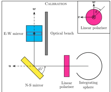
During radiometric and polarimetric calibration, the north– south and east–west scan mirrors will be set at their central positions (θns=π/4 andθew=π/4) so that the instrument
points to nadir along the negativeuaxis, as shown
The Stokes vector after reflection from the north–south mirror will be
S1=R(η1)B(φ1)A(p1, q1)L(θ )S0, (14)
whereS0=(I0,0,0,0)Tis the Stokes vector for unpolarised
light leaving the integrating sphere,
L(θ )=1 2
1 c s 0
c c2 cs 0
s sc s2 0
0 0 0 0
(15)
is the Mueller matrix for the linear polariser inclined at angle
θ, and
c=cos 2θands=sin 2θ. (16)
The plane containing the incident and reflected beams at the east–west mirror is the v–wplane, perpendicular to the corresponding plane for the north–south mirror. Therefore,
η1=π/2 and
R(η1)=
1 0 0 0
0 −1 0 0
0 0 −1 0
0 0 0 1
. (17)
A straightforward calculation yields
S1=I0
4
p12(1+c)+q12(1−c)
−p12(1+c)+q12(1−c)
−2p1q1cosφ1s
−2p1q1sinφ1s
. (18)
The Stokes vector leaving the east–west mirror and arriv-ing at the entrance aperture of the telescope is
S2=R(η2)B(φ2)A(p2, q2)S1. (19)
In the calibration configuration no rotation occurs between the east–west scan mirror and the telescope/spectrograph as-sembly, soη2=0 and the matrixR(η2)is the identity. Thus,
Eq. (19) reduces to
S2=I0 4
p22q12(1−c)+q22p12(1+c) p22q12(1−c)−q22p12(1+c)
−2p1q1p2q2cos(φ1−φ2)s
−2p1q1p2q2sin(φ1−φ2)s
, (20)
while the intensity component of the Stokes vector incident upon the detector will be
I3=
I0
4
m00
h
p22q12(1−c)+q22p12(1+c)i
+m01 h
p22q12(1−c)−q22p21(1+c) i
−2m02p1q1p2q2cos(φ1−φ2)s
−2m03p1q1p2q2sin(φ1−φ2)s
, (21)
with corresponding output potentialvfrom the detector
v=g(I3). (22)
In practice the linear polariser will be set at angles
0=θ1< θ2<· · ·< θn=π/2, (23)
and for each angle the output potential will be measured as the incident intensityI0is stepped over the range likely to be
encountered by geoCARB in space,
I01< I02<· · ·< I0k. (24)
Thus, for angleθi and incident intensityI0j, there will be
a corresponding output potential
vij=g(I0j, θi, m00, m01, m02, m03). (25)
Provided that the north–south and east–west scan mirrors have been characterised well, thenk measurements of vij
will provide an over-determined system of equations for the elementsm00,m01,m02 andm03 of the Mueller matrix as
well as the parameters (such asg0,g1andg2) that define the
functiong. Solution of the over-determined system in a least-squares sense will characterise both the polarimetric and ra-diometric sensitivity of the spectrograph from the entrance aperture of the telescope through to the output from the de-tector.
It is important to note the role played by the phase delays
φ1andφ2in Eq. (21). Ifφ1≈φ2, as is likely to be the case
with similar coatings on the mirrors, thenm03will be difficult
to determine because its coefficient in Eq. (21) will be close to zero. That might not be a serious problem in practice, be-cause the surface and atmosphere generate very little circular polarisation. However, if necessary, a well-characterised re-tarder could be introduced to the calibration set-up between the integrating sphere and the linear polariser to ensure a sig-nificant component of circular polarisation, thereby leading to a more accurate determination ofm03. These matters will
be addressed during the phase A study for geoCARB. Once geoCARB is in flight, the stability of the polarimetric calibration will be monitored using observations of sunglint in a manner similar to that devised for GOSAT by O’Brien et al. (2013).
4 Simplified configuration
In order to assess the polarisation sensitivity of geoCARB with information presently available, we consider a simpli-fied (and idealised) configuration5in which
5This simplified instrument is likely to be more polarising than
– the mirrors are perfectly reflecting, so thatpi=qi =1,
and the phase delaysφ1andφ2are equal;
– the polarising properties of the telescope/spectrograph assembly are dominated by the grating;
– the intensity reflected from the grating when illuminated with plane-polarised light inclined at angleθ=π/4 to the rulings is the average of the intensities atθ=0 and
θ=π/2.
In practice, the last assumption requires that incident radi-ation linearly polarised parallel to the grating rulings should not produce any diffracted light linearly polarised perpendic-ular to the rulings, and vice-versa. With these assumptions, Eq. (21) for the intensity arriving at the detector during cali-bration with the polariser at angleθreduces to
I =I0
2(m00−m01cos 2θ−m02sin 2θ ), (26) where for notational simplicity we have omitted the subscript fromI3.
4.1 Polarimetric calibration
If we assume that the atmosphere generates little circular po-larisation, then only three parameters are required to charac-terise the instrument, namelym00,m01andm02. In principle
only three measurements are needed to fix their values, which for definiteness we assume to be the responsesI(1),I(2)and
I(3)to unpolarised intensityI0with the linear polariser at
an-gles 0,π/4 andπ/2. Substitution of these angles in Eq. (26) leads to
I(1)=I0(m00−m01)/2, I(2)=I0(m00−m02)/2,
I(3)=I0(m00+m01)/2. (27)
The first and third equations yield
m00−m01=Epandm00+m01=Es, (28)
where the ratios
Ep=2I(1)/I0andEs =2I(3)/I0 (29)
are the absolute efficiencies of the grating for linearly po-larised light parallel and perpendicular to the rulings. Thus, we obtain
m00=(Es+Ep)/2 andm01=(Es−Ep)/2, (30)
showing that the coefficientsm00 andm01 can be expressed
simply in terms of the grating efficiencies measured by the manufacturer. Figure 4 shows the absolute efficiencies of the geoCARB gratings, measured by the manufacturer in the O2
Calbration
Integrating sphere Linear
polariser N-S mirror
45◦
E-W mirror
u
w
Optical bench
N v
w
Linear polariser θ
Figure 3.During calibration, both mirrors will be set to their central
positions withθns=θew=π/4, corresponding to nadir
observa-tion. Unpolarised light from a calibrated integrating sphere will be passed through a linear polariser along the optic axis to the north– south scan mirror. The polariser will be rotated about theuaxis so
that the plane of polarisation makes an angleθwith theu–wplane,
as shown in the upper-right insert. Whenθ=0, the plane of
polar-isation (after reflections) is parallel to the slit; whenθ=π/2, the plane of polarisation is perpendicular to the slit. The output poten-tialv(θ )from the detector will be monitored as a function ofθ.
A-band and the weak CO2band, and predicted in the strong
CO2band and the CO band.
The last assumption concerns the sensitivity of the grating to the U component of the radiation incident upon it. The second of the relations in Eq. (27) shows that
I(2)=(I(1)+I(3))/2−m02I0/2. (31)
Therefore, the requirement thatI(2)should be the average ofI(1) andI(3) forcesm02=0, which completes the
char-acterisation of the simplified spectrograph. Without this re-quirement,m02 could be determined from the measurement I(2).
4.2 In-flight operation
Once in flight, the intensity falling upon the detector of the simplified instrument in response to the Stokes vectorS=
(I, Q, U, V )Tat the top of the atmosphere will be simply
I3=m00I0+m01Q0, (32)
where
I0=I and Q0=cos 2η0Q−sin 2η0U.
The Stokes componentU0does not appear in Eq. (32)
The angle between the reference planes used by the radiative transfer code and the instrument isη0; it is a purely
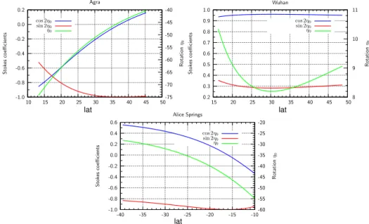
geomet-ric quantity that depends upon the orbit and the scan geome-try. For example, Fig. 5 shows the angleη0for pixels in the
frames through Agra, Wuhan and Alice Springs. The varia-tion inη0is small when the target is close to the longitude of
geoCARB, but elsewhere can be large. If we define
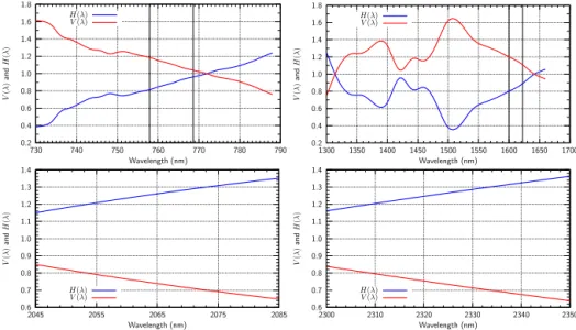
H (λ)= 2Es
Es+Ep
and V (λ)= 2Ep
Es+Ep
,
then Eq. (32) reduces to
I3=m00[I0+(H−V )Q0/2]. (33)
Thus, the intensity reaching the detector for this idealised instrument is identical to that generated by unpolarised in-tensity
I⋆=I0+(H−V )Q0/2 (34)
incident upon the north–south scan mirror.
5 Pseudo measured spectra
An ensemble of spectra were generated for targets in frames passing through Agra, Wuhan and Alice Springs, as de-scribed in Sect. 1. Only land targets were selected for this study because generally the oceans are too dark at the geo-CARB wavelengths.
The meteorology at each target was based on forecasts from the European Centre for Medium-Range Weather Fore-casts (ECMWF), interpolated to the time and location of each observation.6Surface properties were derived from MODIS
and POLDER, which respectively provided the bidirectional reflectance distribution function and polarising properties (Nadal and Breon, 1999). Clouds and aerosols were de-rived from CALIPSO (Cloud-Aerosol Lidar and Infrared Pathfinder Satellite Observations). The vertical profiles of CO2 in the simulator were derived from the Parameterised
Chemical Transport Model (PCTM) (Kawa et al., 2004). For CO, the background profiles were drawn from the Measure-ments of Pollution in the Troposphere (MOPITT) mission (Deeter et al., 2003, 2007a, b). Profiles of CH4 were taken
from a snap-shot of the global CH4 distribution calculated
with the TM5 chemical transport model (Krol et al., 2005). In each case, the profiles were interpolated to the times and locations of the geoCARB observations. Generally the meth-ods were identical to those described by Polonsky et al.
6The specific dates for the simulations were the 21st of March,
June, September and December in 2012. The equinoxes and sol-stices were chosen to capture the seasonal dependence. The only significance of the year 2012 is that data were already on hand for the geophysical variables; we expect similar results for other years. Three observations were simulated for each day, at local solar noon, 3 hours earlier and 3 hours later.
(2014), except that superimposed on the column concentra-tions of CO2, CH4 and CO were random variations drawn
from gaussian distributions with standard deviations of 3.0, 0.1 and 0.01 ppm, respectively. The random variations were added simply to augment the parameter space sampled by the simulations. Similarly, the simulations were performed twice, once with both cloud and aerosol enabled and once with only aerosol, the aim being to generate a larger ensem-ble of “almost clear” scenes with which to test the sensitiv-ity of the retrieval algorithm to polarisation. This approach is reasonable because moderately cloudy scenes are rejected by the algorithm.
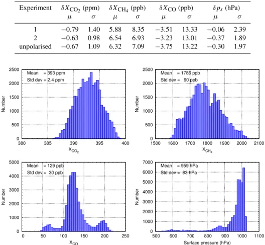
Histograms of surface pressure and the column-averaged concentrations of CO2, CH4and CO are shown in Fig. 7 for
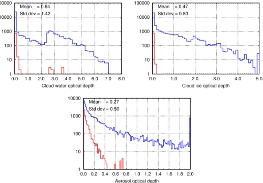
the ensemble of pixels in the frames over Agra, Wuhan and Alice Springs. Figure 8 presents histograms of the optical depth at the O2A-band of cloud liquid water, cloud ice and
aerosol. The histograms in blue represent the entire ensem-ble; those in red show the ensemble members that pass the post-processing filter.
For each target, all components of the Stokes vectorS=
(I, Q, U, V )T were computed at the top of the atmosphere,
with the reference plane for polarisation defined by the lo-cal normal and the direction to the satellite at the target. The spectral channels, their widths and the signal-to-noise ratios were as described for geoCARB by Polonsky et al. (2014). In particular, the instrument line shape functions were assumed to be independent of polarisation. The polarisation model for the idealised instrument was applied to the Stokes vector to calculate the intensity falling upon the detector. As shown earlier, the response of the detector is identical to that pro-duced by unpolarised light at the entrance aperture with in-tensity given by Eq. (34). BecauseHandV depend strongly upon wavelength, the measured spectrum contains an artefact arising from the polarisation sensitivity of the gratings.
The Stokes vectorSwas computed using a three-step
ap-proach: calculate the exact contribution toSfrom first-order
scattering (1OS); calculate the multiply scattered radiance
I at the top of the atmosphere (Ims); calculate the
contri-butions from second-order scattering toQ andU, as well as the polarisation corrections from second-order scattering toI (2OS). By combining the results of these calculations, the Stokes vector at the top of the atmosphere can be es-timated reasonably accurately for nearly clear scenes (Na-traj and Spurr, 2007). The 1OS and 2OS terms used code developed by Natraj and Spurr (2007). Calculation of the first-order component ofI used the TMS (truncated multi-ple scattering) correction of Nakajima and Tanaka (1988), and all three first-order scattering terms include the direct beam scattered from the surface. The multiply scattered in-tensity termIms is calculated using the successive orders of
0 20 40 60 80 100
730 740 750 760 770 780 790
A b so lu te effi ci en cy (% ) Wavelength (nm) parallel perpendicular 0 20 40 60 80 100
1300 1350 1400 1450 1500 1550 1600 1650 1700
A b so lu te effi ci en cy (% ) Wavelength (nm) parallel perpendicular 0 20 40 60 80 100
2045 2055 2065 2075 2085
A b so lu te effi ci en cy (% ) Wavelength (nm) parallel perpendicular 0 20 40 60 80 100
2300 2310 2320 2330 2340 2350
A b so lu te effi ci en cy (% ) Wavelength (nm) parallel perpendicular
Figure 4.Absolute efficiencies of the gratings, measured in the O2A-band and weak CO2band, and predicted in the strong CO2band and
CO band. There are two gratings, each used in two orders of diffraction to serve two bands. The vertical lines define the O2A-band and CO2
weak band. -1.0 -0.8 -0.6 -0.4 -0.2 0.0 0.2
10 15 20 25 30 35 40 45 50-75
-70 -65 -60 -55 -50 -45 -40 S to k es co effi ci en ts R o ta ti o n η0 Agra
cos 2η0 sin 2η0
η0 0.2 0.3 0.4 0.5 0.6 0.7 0.8 0.9 1.0
15 20 25 30 35 40 45 508
9 10 11 S to k es co effi ci en ts R o ta ti o n η0 Wuhan
cos 2η0 sin 2η0
η0 -1.0 -0.8 -0.6 -0.4 -0.2 0.0 0.2 0.4 0.6
-40 -35 -30 -25 -20 -15 -10-60
-55 -50 -45 -40 -35 -30 -25 -20 S to k es co effi ci en ts R o ta ti o n η0 Alice Springs
cos 2η0 sin 2η0
η0
lat lat
lat
Figure 5.Angleη0(right-hand scale) between the reference planes for polarisation used by the radiative transfer code and the geoCARB
instrument, shown as a function of latitude along the frames through Agra, Wuhan and Alice Springs. Also plotted are cos 2η0and sin 2η0
(left-hand scale), which are essentially the Stokes coefficients for the simplified model of the instrument (hence the left-hand label).
(O’Dell et al., 2006). Lastly, the techniques of low-streams interpolation (LSI) developed by O’Dell (2010) was used to compute the Stokes vector on a 0.01 cm−1spectral grid; high accuracy, but widely spaced, radiances were interpolated to the fine spectral grid using a two-stream solver of the radia-tive transfer equation.
Generally, in simulations of this type, random noise would be added to the unpolarised intensity in accordance with the
noise model for geoCARB, and the resulting signal would be regarded as a measurement (or measured spectrum).
However, in this study random noise was not added for the following reason. For every retrieval, differences between the true and retrieved values of the parameters can arise via many mechanisms, including the following:
0.2 0.4 0.6 0.8 1.0 1.2 1.4 1.6 1.8
730 740 750 760 770 780 790
V
(
λ
)
an
d
H
(
λ
)
Wavelength (nm)
H(λ) V(λ)
0.2 0.4 0.6 0.8 1.0 1.2 1.4 1.6 1.8
1300 1350 1400 1450 1500 1550 1600 1650 1700
V
(
λ
)
an
d
H
(
λ
)
Wavelength (nm)
H(λ) V(λ)
0.6 0.7 0.8 0.9 1.0 1.1 1.2 1.3 1.4
2045 2055 2065 2075 2085
V
(
λ
)
an
d
H
(
λ
)
Wavelength (nm)
H(λ) V(λ)
0.6 0.7 0.8 0.9 1.0 1.1 1.2 1.3 1.4
2300 2310 2320 2330 2340 2350
V
(
λ
)
an
d
H
(
λ
)
Wavelength (nm)
H(λ) V(λ)
Figure 6.FunctionsV (λ)andH (λ)for the gratings, measured in the O2A-band and weak CO2band, and predicted in the strong CO2band
and CO band. There are two gratings, each used in two orders of diffraction to serve two bands. The vertical lines define the O2A-band and
CO2weak band.
Table 1. Coefficients in the linear approximations to H (λ)and
V (λ). Wavelengthλis assumed in nm.
Band α(nm−1) β
O2A-band 0.01439 −10.825
Weak CO2band 0.00389 −6.426
Strong CO2band 0.00501 −10.095
CO band 0.00404 −9.118
2. the influence of the prior and algorithm controls, such as the stopping condition;
3. random noise added to the simulated spectra.
The last source is the most understood, and its magnitude can be quantified easily by the posterior uncertainties returned by the retrieval algorithm, the calculation of which uses the in-strument signal-to-noise ratio. Furthermore, random noise in the spectra generally will not cause a bias, because the ra-diative transfer problem can be linearised in the vicinity of the true solution. Consequently, we can concentrate on the biases introduced by factors other than random noise (such as the first two items listed above). Since the model errors and the random noise (items 1 and 3) are statistically inde-pendent, including the effects of random noise simply widens the bias distribution by the width of the random uncertainty. As the focus of this study is the bias introduced by polari-sation effects, it was judged that the effects would be easier to spot in the narrower error distributions calculated without random noise.
6 Trace gas recovery
Optimal estimation was used to match “measured” (in reality simulated) and modelled spectra, as described by Polonsky et al. (2014) for the baseline configuration of geoCARB. In addition to the trace gas (CO2, CH4and CO) concentrations,
the state vector contained many other parameters describing the surface, the atmosphere and the scattering properties of aerosol and cloud. All were adjusted iteratively during the matching process.
Table 2.Means (µ) and standard deviations (σ) of the biasesδXCO2,δXCH4,δXCOandδps in retrievedXCO2,XCH4,XCOand surface pressure from the two experiments. The row labelled “unpolarised” contains reference results obtained for an instrument equipped with ideal polarisation scramblers.
Experiment δXCO2(ppm) δXCH4(ppb) δXCO(ppb) δps(hPa)
µ σ µ σ µ σ µ σ
1 −0.79 1.40 5.88 8.35 −3.51 13.33 −0.06 2.39
2 −0.63 0.98 6.54 6.93 −3.23 13.01 −0.37 1.89
unpolarised −0.67 1.09 6.32 7.09 −3.75 13.22 −0.30 1.97
0 500 1000 1500 2000 2500
380 385 390 395 400
Number
XCO
2 Mean = 393 ppm
Std dev = 2.4 ppm
0 500 1000 1500 2000 2500
1500 1600 1700 1800 1900 2000 2100
Number
XCH
4 Mean = 1786 ppb
Std dev = 90 ppb
0 1000 2000 3000 4000 5000
0 50 100 150 200 250
Number
XCO
Mean = 129 ppb
Std dev = 30 ppb
0 1000 2000 3000 4000 5000 6000 7000
500 600 700 800 900 1000 1100
Number
Surface pressure (hPa) Mean = 959 hPa
Std dev = 83 hPa
Figure 7. Histograms ofXCO2,XCH4,XCOand surface pressure for the ensemble of soundings in the simulation. The surface pressure
histogram covers a wide range because the frame passing through Agra includes the Himalaya.
cloud could differ significantly from the aerosol and cloud from CALIPSO used in the simulation of the measured spec-tra, again breaking the circularity of the simulation-retrieval process.
For each day, each observation time and each (approxi-mately) north–south scan line (through Agra, Wuhan or Alice Springs), the prior profile of CO2was taken to be the average
of the profiles at all of the target pixels along the scan line. This was judged to be a fair prior, neither too optimistic nor too pessimistic, and indicative of the accuracy possible with large-scale averages predicted by general circulation models. Prior profiles of CH4and CO were calculated similarly.
At the completion of the optimal estimation, a post-processing filter (PPF) is applied to reject cases where the model approximation to the spectra is poor. This may hap-pen for many reasons, but the majority of cases occur when the optical properties assumed for aerosol and cloud do not match those used to simulate the spectra. The experiments in this study used the same PPF as Polonsky et al. (2014). The PPF checksχ2in the bands used to retrieveXCO2, the
retrieved aerosol optical depth at the blue end of the O2
A-band and the number of degrees of freedom for signal in the retrieved profile of CO2. Each check involves comparison
with a fixed, preset threshold. If any check fails, the scene is rejected. Only results that pass the PPF are shown.
The functionsH (λ)andV (λ)derived from the efficiencies of the gratings to polarisations parallel and perpendicular to the slits were approximated by linear functions, which take the form
H=αλ+β+1 and V = −αλ−β+1
becauseH+V =2 by definition. The coefficientsαandβ
1 10 100 1000 10000 100000
0.0 1.0 2.0 3.0 4.0 5.0 6.0 7.0 8.0
Cloud water optical depth Mean = 0.84
Std dev = 1.42
1 10 100 1000 10000 100000
0.0 1.0 2.0 3.0 4.0 5.0
Cloud ice optical depth Mean = 0.47
Std dev = 0.80
1 10 100 1000 10000
0.0 0.2 0.4 0.6 0.8 1.0 1.2 1.4 1.6 1.8 2.0
Number
Aerosol optical depth Mean = 0.27
Std dev = 0.50
Figure 8.Histograms of the optical depth of cloud liquid water, cloud ice and aerosol for the ensemble of soundings in the simulation. The
histograms in blue refer to the whole ensemble; those in red apply after the post-processing filter.
0.12 0.14 0.16 0.18 0.20 0.22 0.24 0.26 0.28
757 759 761 763 765 767 769
Degree of polarisation
Wavelength (nm)
Cloud disabled Mean
Std dev
0.06 0.08 0.10 0.12 0.14 0.16 0.18 0.20
757 759 761 763 765 767 769
Degree of polarisation
Wavelength (nm)
Cloud enabled Mean
Std dev
Figure 9.Mean and standard deviation of the degree of polarisation simulated at the top of the atmosphere in the O2A-band. In the left-hand
panel the soundings with cloud were discarded, so the sources of polarisation are the surface and scattering by aerosols and molecules. The right-hand panel applies to soundings with cloud.
6.1 Experiment 1
In the first experiment, the measured spectrum was taken to beI⋆as defined in Eq. (34). Knowledge ofHandV was de-nied to the retrieval algorithm, so it attempted to matchI⋆ us-ing only the intensity at the top of the atmosphere. Thus, the measured spectrum contains not only the intensity but also the slowly varying wavelength dependence of(H−V ), upon which is superimposed the rapid wavelength dependence of
Q0, while the retrieval algorithm attempts to fit the measured
spectrum with the intensity. In a sense this experiment rep-resents the worst case, because it assumes that no pre-flight polarimetric calibration has been performed.
The degree of polarisation, defined by
P=pQ2+U2+V2/I, (35)
varies strongly across the absorption spectrum, peaking at the line centres and falling to a backgroud level, determined principally by the surface and Rayleigh scattering, in the con-tinuum between the lines. At wavelengths in the cores of the lines, photons are likely to have been scattered higher in the atmosphere by molecules, clouds and aerosols, which typi-cally have stronger polarisation signatures than the surface. Figure 9 shows the mean and standard deviation of the degree of polarisation in the O2A-band for the ensemble of
0 100 200 300 400 500
-4 -3 -2 -1 0 1 2 3 4
Number
XCO2 bias (ppm)
Mean1 = -0.79 ppm
Std dev1 = 1.40 ppm
Mean2 = -0.63 ppm
Std dev2 = 0.98 ppm
0 50 100 150 200 250
-30 -20 -10 0 10 20 30
Number
XCH4 bias (ppb)
Mean1 = 5.9 ppb
Std dev1 = 8.4 ppb
Mean2 = 6.5 ppm
Std dev2 = 6.9 ppm
0 100 200 300 400 500
-50 -40 -30 -20 -10 0 10 20 30 40 50
Number
XCO bias (ppb)
Mean1 = -3.5 ppb
Std dev1 = 13.3 ppb
Mean2 = -3.2 ppb
Std dev2 = 13.0 ppb
0 100 200 300 400
-10 -5 0 5 10
Number
Surface pressure bias (hPa)
Mean1 = -0.06 hPa
Std dev1 = 2.39 hPa
Mean2 = -0.37 hPa
Std dev2 = 1.89 hPa
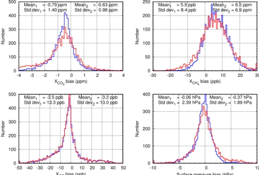
Figure 10.Histograms of the biases inXCO2,XCH4,XCOand surface pressure for the ensemble of soundings in the simulation. The red and
blue histograms apply to Experiments 1 and 2, respectively.
-200 -150 -100 -50 0 50 100 150
-200 -150 -100 -50 0 50
Retrieved albedo slope (cm)
True albedo slope (cm) O2 A-band
-200 -150 -100 -50 0 50 100 150
-200 -150 -100 -50 0 50
Retrieved albedo slope (cm)
True albedo slope (cm) O2 A-band
Figure 11.Correlations between true and retrieved albedo slope in the O2A-band. The slopes (in units (cm−1)−1or cm) have been multiplied
by 106. The left-hand panel is for an instrument equipped with ideal polarisation scramblers; the right-hand panel applies to Experiment 2
for geoCARB.
the surface and by scattering from aerosols and molecules, but not from clouds. The right-hand panel applies to the en-semble with cloud enabled.
6.2 Experiment 2
In the second experiment, the retrieval algorithm was given access to the instrument Mueller matrix, which for the sim-plified instrument amounts to knowing the functionsH and
V derived from the grating efficiencies. Thus, the retrieval al-gorithm computesI0+(H−V )Q0/2 and uses this to match
the measured spectrum. We stress, however, that the retrieval algorithm assumes a non-polarising, Lambertian surface and fixed types of aerosol and cloud whose scattering properties are specified, so its ability to reproduce the measured Stokes vector at the top of the atmosphere is limited.
For reference, the results of this experiment are compared with those from an instrument with an ideal polarisation scrambler, where the measured spectrum is the intensity and the retrieval algorithm attempts to fit the measured spectrum with its internally generated representation of the intensity.
7 Results
Histograms of the biases in retrievedXCO2,XCH4,XCOand
The effect of ignoring the polarising properties of the grat-ings is apparent in the histograms of Fig. 10. The histograms for retrievedXCO2and surface pressure are broader, with
out-liers well beyond the targets set for the geoCARB mission. The impact on retrieved XCH4 andXCOis smaller, for
rea-sons presently unknown, but is still significant. While the differences in the average biases shown in Table 2 appear small, they nevertheless are important, because even small biases on large spatial scales can lead to significant errors in surface fluxes of CO2.
Figure 10 shows that the retrieval algorithm can account for the spectral slope introduced by the gratings, provided that the spectrographs are calibrated before launch. However, there are hidden side effects. For example, the slopes of the surface albedos across the spectral bands of geoCARB, re-trieved simultaneously with the gas concentrations, are not as accurate as for the idealised, unpolarised case. This is demonstrated in Fig. 11 for the slope on the O2 A-band
albedo. The upper panel shows the correlation between the true and retrieved slopes for the unpolarised case. The cor-relation is tight, indicating that this parameter is well deter-mined. The lower panel is for Experiment 2 with geoCARB. Although the functionsV (λ)andH (λ)have been supplied to the retrieval algorithm, and although the trace gas concen-trations have been retrieved well, there clearly is ambiguity in the slope of the albedo. Because the aim of geoCARB is to retrieve trace gas concentrations, this ambiguity is not a seri-ous concern.
8 Conclusions
In this study column-averaged concentrations of CO2 were
retrieved from spectra measured at the top of the atmosphere by a geoCARB-like instrument. The ability of the retrieval algorithm to predict the polarisation state is limited because internally it assumes that the surface is non-polarising and Lambertian and that aerosols and clouds are composed from fixed types whose scattering (and polarising) properties are assigned, fixed and usually inconsistent with the real atmo-sphere. This inability leads to an irreducible minimum error when the algorithm is applied to a realistic ensemble of sur-faces and atmospheres.
For an instrument that is sensitive to the degree of polar-isation, rather than just to the radiant intensity, the error in retrieved trace gas concentrations is expected to be larger. The reason is that the retrieval algorithm will have difficulty matching the measured spectrum, which is a linear combina-tion of the elementsI,Q,UandV of the Stokes vector with coefficients (Stokes coefficients) that are specific to the in-strument and the viewing geometry. The Stokes coefficients generally vary slowly with wavelength, though the changes over a band may be large. Thus, the measured spectrum will mix the slow wavelength variation of the Stokes coefficients with the rapid variation inherited from the Stokes
compo-nents. Unless the retrieval algorithm can imitate this wave-length dependence, errors in XCO2,XCH4 andXCO can be
expected.
The experiments in this study show that errors caused by unknown polarisation do arise. However, generally they are small, though they remain significant forXCO2. They are not
disastrous because the retrieval algorithm allows the surface albedo to vary linearly with wavelength over each band, and it adjusts the slope during the retrieval. This adjustment of surface albedo with wavelength compensates to a large de-gree for the wavelength dependence of the Stokes coeffi-cients. Thus, even in the presence of significant polarisation at the entrance aperture, geoCARB should recover reliable estimates for both trace gas concentrations and the band-averaged surface albedo, but it might assign the slope of the surface albedo incorrectly.
Through radiometric and polarimetric calibration before launch using the procedure defined in this study, errors from polarised surfaces and clouds can be reduced to negligible levels compared with other systematic biases in the retrieval algorithm. If in the future the latter can be reduced, then po-larisation biases would need to be re-examined.
Acknowledgements. Polonsky was supported by a contract from Lockheed Martin Advanced Technology Center, Palo Alto, for this work. The retrieval algorithm was adapted by Polonsky from the ACOS algorithm developed for GOSAT by NASA’s ACOS team, whose excellent work we gratefully acknowledge. The retrieval algorithm was run on the OCO cluster at Colorado State University, thanks to support from Chris O’Dell. The code that generated geoCARB spectra was written and run in Melbourne on the 16-node cluster at Greenhouse Gas Monitor Australia Pty. Ltd.
Edited by: F. Hase
References
Deeter, M. N., Emmons, L. K., Francis, G. L., Edwards, D. P., Gille, J. C., Warner, J. X., Khattatov, B., Ziskin, D., Lamar-que, J.-F., Ho, S.-P., Yudin, V., Attié, J.-L., Packman, D., Chen, J., Mao, D., and Drummond, J. R.: Operational carbon monoxide retrieval algorithm and selected results for the MOPITT instru-ment, J. Geophys. Res., 108, 4399, doi:10.1029/2002JD003186, 2003.
Deeter, M. N., Edwards, D. P., and Gille, J. C.: Retrievals of carbon monoxide profiles from MOPITT observations using lognormal a priori statistics, J. Geophys. Res., 112, 11311, doi:10.1029/2006JD007999, 2007a.
Deeter, M. N., Edwards, D. P., Gille, J. C., and Drummond, J. R.: Sensitivity of MOPITT observations to carbon monoxide in the lower troposphere, J. Geophys. Res., 112, 24306, doi:10.1029/2007JD008929, 2007b.
Kawa, S. R., Erickson, D. J., Pawson, S., and Zhu, Z.: Global
CO2 transport simulations using meteorological data from the
NASA data assimilation system, J. Geophys. Res., 109, 18312, doi:10.1029/2004JD004554, 2004.
Krol, M., Houweling, S., Bregman, B., van den Broek, M., Segers, A., van Velthoven, P., Peters, W., Dentener, F., and Bergamaschi, P.: The two-way nested global chemistry-transport zoom model TM5: algorithm and applications, Atmos. Chem. Phys., 5, 417– 432, doi:10.5194/acp-5-417-2005, 2005.
Kumer, J. B., Rairden, R. L., Roche, A. E., Chevallier, F., Rayner, P. J., and Moore, B.: Progress in development of Tro-pospheric Infrared Mapping Spectrometers (TIMS): geoCARB green house gas (GHG) application, Proc. SPIE, 8867, 88670K, doi:10.1117/12.2022668, 2013.
Mishchenko, M. I., Travis, L. D., and Lacis, A. A.: Scattering, Ab-sorption, and Emission of Light by Small Particles, Cambridge University Press, Cambridge, UK, 2002.
Mobilia, J., Kumer, J. B., Palmer, A., Sawyer, K., Mao, Y., Katz, N., Mix, J., Nast, T., Clark, C. S., Vanbezooijen, R., Magoncelli, A., Baraze, R. A., and Chenette, D. L.: Determination of technical readiness for an atmospheric carbon imaging spectrometer, Proc. SPIE, 8867, 88670L, doi:10.1117/12.2029634, 2013.
Nadal, F. and Breon, F.-M.: Parameterization of surface
po-larized reflectance derived from POLDER spaceborne
measurements, IEEE T. Geosci. Remote, 37, 1709–1718, doi:10.1109/36.763292, 1999.
Nakajima, T. and Tanaka, M.: Algorithms for radiative inten-sity calculations in moderately thick atmospheres using a trun-cation approximation, J. Quant. Spectrosc. Ra. 40, 51–69, doi:10.1016/0022-4073(88)90031-3, 1988.
Natraj, V. and Spurr, R. J. D.: A fast linearized pseudo-spherical two orders of scattering model to account for polarization in vertically inhomogeneous scattering-absorbing media, J. Quant. Spectrosc. Ra., 107, 263–293, doi:10.1016/j.jqsrt.2007.02.011, 2007.
O’Brien, D. M., Polonsky, I., O’Dell, C., Kuze, A., Kikuchi, N., Yoshida, Y., and Natraj, V.: Testing the polarization model for TANSO-FTS on GOSAT against clear-sky observations of sun-glint over the ocean, IEEE T. Geosci. Remote, 51, 5199–5209, doi:10.1109/TGRS.2012.2232673, 2013.
O’Dell, C., Heidinger, A. K., Greenwald, T., Bauer, P., and Ben-nartz, R.: The successive-order-of-interaction radiative transfer model: Part II: Model performance and applications, J. Appl. Meteorol. Clim., 45, 1403–1413, doi:10.1175/JAM2409.1, 2006. O’Dell, C. W.: Acceleration of multiple-scattering, hyperspectral radiative transfer calculations via low-streams interpolation, J. Geophys. Res., 115, D10206, doi:10.1029/2009JD012803, 2010. Polonsky, I. N., O’Brien, D. M., Kumer, J. B., O’Dell, C. W., and the geoCARB Team: Performance of a geostationary mission,
geoCARB, to measure CO2, CH4and CO column-averaged
con-centrations, Atmos. Meas. Tech., 7, 959–981, doi:10.5194/amt-7-959-2014, 2014.
Rayner, P. J., Utembe, S. R., and Crowell, S.: Constraining re-gional greenhouse gas emissions using geostationary concentra-tion measurements: a theoretical study, Atmos. Meas. Tech., 7, 3285–3293, doi:10.5194/amt-7-3285-2014, 2014.
Sawyer, K., Clark, C., Katz, N., Kumer, J., Nast, T., and Palmer, A.: GeoCARB design maturity and geostationary heritage, Proc. SPIE, 8867, 88670M, doi:10.1117/12.2024457, 2013.