www.solid-earth.net/5/673/2014/ doi:10.5194/se-5-673-2014
© Author(s) 2014. CC Attribution 3.0 License.
Using the Nordic Geodetic Observing System for land uplift studies
M. Nordman1, M. Poutanen1, A. Kairus1,2, and J. Virtanen1 1Finnish Geodetic Institute, P.O. Box 15, 02431 Masala, Finland 2Aalto University, Espoo, Finland
Correspondence to:M. Nordman ([email protected])
Received: 9 January 2014 – Published in Solid Earth Discuss.: 30 January 2014 Revised: 12 May 2014 – Accepted: 13 May 2014 – Published: 17 July 2014
Abstract. Geodetic observing systems have been planned and developed during the last decade. An ideal observing system consists of a network of geodetic observing stations with several techniques at the same site, publicly accessible databases, and as a product delivers data time series, combi-nation of techniques or some other results obtained from the data sets. Globally, there is the International Association of Geodesy (IAG) Global Geodetic Observing System (GGOS), and there are ongoing attempts to create also regional observ-ing systems. In this paper we introduce one regional system, the Nordic Geodetic Observing System (NGOS) hosted by the Nordic Geodetic Commission (NKG).
Data availability and accessibility are one of the major is-sues today. We discuss in general data-related topics, and introduce a pilot database project of NGOS. As a demon-stration of the use of such a database, we apply it for post-glacial rebound studies in the Fennoscandian area. We com-pare land uplift values from three techniques, GNSS, tide gauges and absolute gravity, with the Nordic Geodetic Com-mission NKG2005LU land uplift model for Fennoscandia. The purpose is to evaluate the data obtained from different techniques and different sources and get the most reliable values for the uplift using publicly available data.
The primary aim of observing systems will be to produce data and other products needed by multidisciplinary projects, such as Upper Mantle Dynamics and Quaternary Climate in Cratonic Areas (DynaQlim) or the European Plate Observ-ing System (EPOS), but their needs may currently exceed the scope of an existing observing system. We discuss what re-quirements the projects pose to observing systems and their development. To make comparisons between different stud-ies possible and reliable, the researcher should document what they have in detail, either in appendixes, supplementary material or some other available format.
1 Introduction
Permanent geodetic observing networks have been devel-oped during the last decade to become the basic component of geodetic observing systems. The observing systems aim to provide better and more detailed information on the global and regional gravity field, its temporal variation, crustal de-formation, global changes in Earth’s shape, mass distribu-tion, sea level, and the Earth orientation in the inertial frame. An ideal observing system consists of geodetic observing sta-tions with several techniques at the same site, publicly acces-sible databases, and as products, data and combination of dif-ferent observing techniques. An ideal observing system also has a carefully documented database, where all information related to measurements, modelling, products and other sub-tleties is stored.
Globally, the International Association of Geodesy Global Geodetic Observing System (IAG GGOS) is based on ex-isting IAG Service; see (http://www.iag-aig.org/) for details and access points to the services and their products. Status and goals are described in Plag and Pearlman (2009). Par-allel to the development of GGOS, regional systems have been discussed and initiated. These include the European Combined Geodetic Network (ECGN) by the IAG Reference Frame Sub-Commission 1.3a for Europe (EUREF; Ihde et al., 2004; Poutanen et al., 2014), and the Nordic Geodetic Observing System (NGOS) of the Nordic Geodetic Commis-sion (NKG; Poutanen et al., 2005, 2007).
data, whereas the observed gravity change is the sum of mass and height changes. The combination of techniques can verify results of a single technique and help to quantify uncertainties between the techniques and help us to under-stand physical processes behind changes (e.g. Poutanen et al., 2010).
There are several ongoing initiatives which need such high-quality multi-technique data. As an example, we men-tion two: Upper Mantle Dynamics and Quaternary Climate in Cratonic Areas (DynaQlim; Poutanen et al., 2010), and Eu-ropean Plate Observing System (EPOS; http://www.epos-eu. org/). EPOS is an integrated solid Earth sciences research infrastructure approved by the European Strategy Forum on Research Infrastructures (ESFRI) and included in the ESFRI Roadmap. DynaQlim is a regional coordination committee of the International Lithosphere Program (ILP) and studies up-per mantle dynamics, its composition and physical proup-perties (temperature and rheology), and Quaternary climate primar-ily on Fennoscandia, northern Canada and Antarctica.
Specific data needs of such research may exceed the scope of an existing observing system, and this raises the issue of observing system product development. As an example of such dialogue, a joint meeting of GGOS and DynaQlim was organized in 2009 in Espoo, Finland (Gross and Poutanen, 2009). One of the goals was to discuss what specific data or products DynaQlim may expect from GGOS and what pos-sibilities GGOS has to fulfill such requirements. An obvious shortcoming of GGOS is the density of the observing net-work. It is too sparse for regional studies, and there is a need for denser regional observing networks.
One of the major geodynamic processes acting in Fennoscandia and northern Canada is the land uplift caused by glacial isostatic adjustment (GIA). GIA is the response of the solid Earth to the time-varying load due to the waxing and waning of glaciers, causing sea level to vary by up to 130 m in cycles of∼100 000 years. Taking into account the mass change between oceans and glaciers and upper man-tle viscoelastic flow, there is a total of 5×10¹⁹kg of mass transportation during the glaciation cycle (almost 10−5of the
mass of the Earth; e.g. van Dam et al., 2008; Poutanen and Ivins, 2010).
The GIA signal, however, is contaminated by non-GIA-induced mass changes and crustal deformation. Separating GIA-induced contributions from other sources is not straight-forward and using data from a geodetic observing system with multiple techniques can help in this task. However, the global network of GGOS is not sufficient to observe GIA in detail because in the Fennoscandian rebound area there are only half a dozen GGOS stations. In northern Canada, the number of stations is even smaller.
An improvement is to include permanent stations of a regional network. In Fennoscandia, there exists the NGOS network, which contains the Nordic geodetic permanent GPS/GNSS stations (Poutanen et al., 2005, 2007) operated by the national mapping authorities. Mass change can be
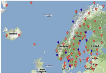
es-Figure 1.The stations in the NGOS database. The blue dots show
the stations chosen for the comparison (see text, names of stations are shown in Fig. 3). Map: Google.
timated from the gravity change which is monitored by re-peated measurements by absolute gravimeters and combined with the height change data given by GPS. A step further is the EPOS which is planned to be an open access infras-tructure serving as primary source of data and tools for re-searchers in geosciences (http://www.epos-eu.org/).
It is important to test the capability of current observing systems and regional networks, databases and other sources of information in GIA-related studies. The EUREF Tech-nical Working Group decided in 2011 to propose a pilot project within the ECGN (Poutanen et al., 2014). The project is meant to demonstrate the ideas and usefulness of a re-gional observing system in utilizing existing networks and databases. The ECGN network consists mostly of EPN (EU-REF Permanent GNSS Network) stations, which especially in Fennoscandia are too sparse for detailed studies of re-gional crustal deformation.
A suitable network for such studies already exists in Fennoscandia as a result of the NKG NGOS task force in the period 2004–2010 (Poutanen et al., 2005, 2007) and its follow-on pilot project Nordic Combined Geodetic Network (NCGN).
As a part of the NCGN project, we have collected informa-tion of geodetic stainforma-tions in the Fennoscandian and Baltic ar-eas into a database using mostly the NGOS stations (Kairus, 2012). We describe the data in Sect. 2, comparison of dif-ferent techniques and discussion of results are presented in Sect. 3, and Sect. 4 is left for conclusions.
2 Selection of data and previously published studies
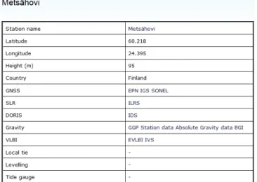
Figure 2.Database entry for station Metsähovi, containing station
coordinates, and links to various databases with observations from Metsähovi.
NKG web pages (http://www.nkg.fi → NKG Data Banks). The station list database is also available as a clickable map interface (Fig. 1). For each station a page with sta-tion informasta-tion and links to relevant databases was created (Fig. 2). The links include GNSS databases (The Interna-tional GNSS Service (IGS; http://igscb.jpl.nasa.gov/), EU-REF Permanent Network (EPN; http://www.epncb.oma.be/) and SONEL (http://www.sonel.org)), gravity databases in the Global Geodynamics Project (GGP; http://www.eas.slu.edu/ GGP/ggphome.html) and the International Gravimetric Bu-reau (BGI; http://bgi.omp.obs-mip.fr/), tide gauge databases in the Permanent Service for Mean Sea Level (PSMSL; http://www.psmsl.org/) and SONEL, and databases of VLBI (Very Long Baseline Interferometry), SLR (Satellite Laser Ranging) and DORIS (Doppler Orbitography and Radiopo-sitioning Integrated by Satellite) of respective IAG/GGOS services (http://www.ggos.org/ →Products). In addition to data, links to relevant research papers are given.
To demonstrate and study the usefulness of the database to study GIA-induced land uplift, we have chosen 12 sta-tions. They are all located at the coast, have permanent GNSS stations with absolute gravity measurements and are in the vicinity of a tide gauge. The locations are shown in Fig. 1 with blue dots.
There have been numerous campaigns and observations in Fennoscandia for land uplift studies using different tech-niques together and separately. Land uplift data from several previously published sources are collected here but there are several nuisances which are not properly handled. For exam-ple, tide gauge heights are orthometric, whereas GNSS refer to the ellipsoidal heights. Different techniques refer to dif-ferent points, for example GNSS height refers either to the antenna or a benchmark on the ground whereas gravity is measured on a different point. Local ties are incomplete at
most stations. A step forward was taken in the first science week of NKG in Reykjavik, March 2013, where its devel-opment was decided and then taken in use by the working groups of the NKG.
2.1 GNSS data
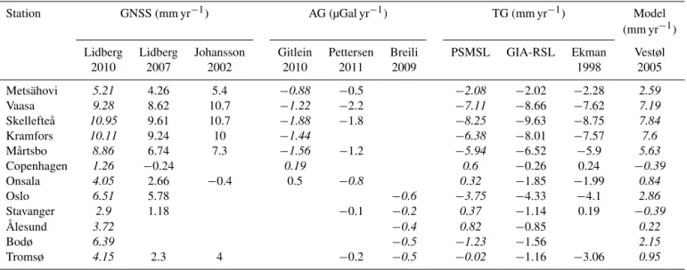
GNSS provides three-dimensional coordinates, where the station height is given above the ellipsoid. The time series and land uplift rates derived from the BIFORST (Baseline Inferences for Fennoscandian Rebound, Sea-level, and Tec-tonics) GPS studies have the densest spatial coverage of all techniques at the moment. The stations have been operational since the mid-1990s, thus offering time series of almost 20 years. There are several studies published, the first one by Johansson et al. (2002). The next generation of uplift rates were published in Lidberg et al. (2007), and the latest update in Lidberg et al. (2010). Uplift rates from GNSS time series can be seen in the first part of Table 1. We have chosen the results of Lidberg et al. (2010) (in italic in Table 1) for the comparison because the time series are the longest (maxi-mum 10.2 years) and the spatial coverage (with 85 stations) is the largest. GNSS processing software has been markedly developed, making it possible to recompute satellite orbits in a unified reference frame and, in turn, giving a more con-sistent solution over the years. These are also in favour of choosing the latest solution. Uncertainty of the uplift value based on the GNSS time series depends mostly on the length of time series; temporal correlations may cause the error to reduce slower. For stations with long time series, the uncer-tainty is 0.2 mm yr−1, whereas for other stations the uncer-tainty is approximately 0.5 mm yr−1(Lidberg et al., 2010).
2.2 Absolute gravity data
Gravity changes provide information on mass changes re-lated to the land uplift. The gravity change can be converted to height change by using a simple ratio, limited by theoreti-cally computed bounds, and derived from observations:
˙
g/h˙= −0.17µGal mm−1, (1)
whereg˙is the gravity change andh˙is the height change (e.g. Ekman and Mäkinen, 1996). The ratio has been evaluated from different data sets yielding slightly different values, e.g. −0.163±0.02 (Gitlein, 2010),−0.16 and−0.20 µGal mm−1 (Mäkinen et al., 2005). Our value falls within this range.
Table 1.Trend estimates of all techniques and different sources for the selected sites (see Fig. 1). AG is absolute gravity, TG is tide gauge.
In italic are the values chosen for each station for comparison. Model is the NKG2005LU uplift model.
Station GNSS (mm yr−1) AG (µGal yr−1) TG (mm yr−1) Model
(mm yr−1)
Lidberg Lidberg Johansson Gitlein Pettersen Breili PSMSL GIA-RSL Ekman Vestøl
2010 2007 2002 2010 2011 2009 1998 2005
Metsähovi 5.21 4.26 5.4 −0.88 −0.5 −2.08 −2.02 −2.28 2.59
Vaasa 9.28 8.62 10.7 −1.22 −2.2 −7.11 −8.66 −7.62 7.19
Skellefteå 10.95 9.61 10.7 −1.88 −1.8 −8.25 −9.63 −8.75 7.84
Kramfors 10.11 9.24 10 −1.44 −6.38 −8.01 −7.57 7.6
Mårtsbo 8.86 6.74 7.3 −1.56 −1.2 −5.94 −6.52 −5.9 5.63
Copenhagen 1.26 −0.24 0.19 0.6 −0.26 0.24 −0.39
Onsala 4.05 2.66 −0.4 0.5 −0.8 0.32 −1.85 −1.99 0.84
Oslo 6.51 5.78 −0.6 −3.75 −4.33 −4.1 2.86
Stavanger 2.9 1.18 −0.1 −0.2 0.37 −1.14 0.19 −0.39
Ålesund 3.72 −0.4 0.82 −0.85 0.22
Bodø 6.39 −0.5 −1.23 −1.56 2.15
Tromsø 4.15 2.3 4 −0.2 −0.5 −0.02 −1.16 −3.06 0.95
Table 2.Comparison of uplift trends for different techniques. AG is
absolute gravity converted using formula (1), TG is tide gauge and Model represents the NKG2005LU uplift model values converted to the absolute uplift values using Eq. (2). Here we use the eustatic sea level rise of 1.32 mm yr−1. Mean is the mean value of four
tech-niques and SD is the standard deviation.
Station GNSS AG TG Model Mean SD
Metsähovi 5.21 5.18 3.62 4.16 4.54 0.79
Vaasa 9.28 7.18 8.97 9.05 8.62 0.97
Skellefteå 10.95 11.06 10.18 9.74 10.48 0.63
Kramfors 10.11 8.47 8.19 9.49 9.07 0.89
Mårtsbo 8.86 9.18 7.72 7.39 8.29 0.86
Copenhagen 1.26 −1.12 0.77 0.99 0.47 1.08
Onsala 4.05 4.71 1.06 2.30 3.03 1.66
Oslo 6.51 3.53 5.39 4.45 4.97 1.28
Stavanger 2.90 1.18 1.01 0.99 1.52 0.92
Ålesund 3.72 2.35 0.53 1.64 2.06 1.34
Bodø 6.39 2.94 2.71 3.69 3.93 1.69
Tromsø 4.15 2.94 1.43 2.41 2.73 1.13
of the absolute gravity measurements has been estimated to be±0.3 µGal yr−1(Timmen et al., 2011) for one instrument over 5 years. This corresponds to an error of±1.8 mm yr−1 in the uplift value.
2.3 Tide gauge data
Tide gauges measure the sea level relative to land and provide the longest continuous geodetic time series in the Fennoscan-dia. The water column records start already in 1774 in Stock-holm and there are tide gauges in the area dating back to the end of the 19th century. There are several sources for the tide gauge data; we have used tide gauge trends derived
in Peltier (1998, 2004), Ekman (1998) and Woodworth and Player (2004).
The trends of the Permanent Service for Mean Sea Level (PSMSL, Woodworth and Player, 2004) are the apparent mean sea level secular trends derived from PSMSL data with all available observations for each station. These trends were updated in 2014 and refer to the revised local ref-erence (RLR; http://www.psmsl.org/products/trends/trends. txt). Glacial isostatic-adjustment-corrected relative sea level trends (GIA-RSL) are the apparent sea level trends predicted from Peltier’s GIA model (Peltier, 1998, 2004). The third set of trends are the values from Ekman (1998), which combine levelling and tide gauge data to define the sea level rise. We choose the PSMSL secular trends for the present comparison (Table 1), because they are not affected by other techniques (e.g. GIA model or fitting of data).
There are three different cases of uplift values which can be observed. From the GNSS time series one obtains the ab-solute uplift: height change of the crust relative to the mass centre of the Earth (origin of the global reference frame). With a tide gauge, one observes the apparent uplift value, i.e. change of the sea level relative to the shoreline. The relative uplift is the difference of the apparent uplift rates between two tide gauges. The apparent uplift differs from the abso-lute uplift due to the global eustatic sea level rise, rise of the geoid, as well as steric effects (salinity and density changes due to the thermal expansion). The relation between these is (Mäkinen et al., 2005)
˙
h= ˙Ha+ ˙He+ ˙N+ ˙Hs, (2) whereh˙is the absolute uplift rate,H˙a is the apparent uplift,
˙
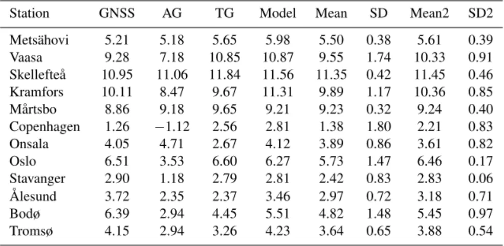
Table 3.Comparison of uplift trends for different techniques. AG is absolute gravity converted using formula (1), TG is tide gauge and Model
represents the NKG2005LU uplift model values converted to the absolute uplift values using Eq. (2). We use here the eustatic sea level rise of 3.11 mm yr−1. Mean is the mean value of four techniques and SD is the standard deviation. Mean2 and SD2 are computed without the
absolute gravity values (see text).
Station GNSS AG TG Model Mean SD Mean2 SD2
Metsähovi 5.21 5.18 5.65 5.98 5.50 0.38 5.61 0.39
Vaasa 9.28 7.18 10.85 10.87 9.55 1.74 10.33 0.91
Skellefteå 10.95 11.06 11.84 11.56 11.35 0.42 11.45 0.46
Kramfors 10.11 8.47 9.67 11.31 9.89 1.17 10.36 0.85
Mårtsbo 8.86 9.18 9.65 9.21 9.23 0.32 9.24 0.40
Copenhagen 1.26 −1.12 2.56 2.81 1.38 1.80 2.21 0.83
Onsala 4.05 4.71 2.67 4.12 3.89 0.86 3.61 0.82
Oslo 6.51 3.53 6.60 6.27 5.73 1.47 6.46 0.17
Stavanger 2.90 1.18 2.79 2.81 2.42 0.83 2.83 0.06
Ålesund 3.72 2.35 2.37 3.46 2.97 0.72 3.18 0.71
Bodø 6.39 2.94 4.45 5.51 4.82 1.48 5.45 0.97
Tromsø 4.15 2.94 3.26 4.23 3.64 0.65 3.88 0.54
In Tables 2 and 3, the tide gauge values are corrected for the eustatic sea level rise using two different estimates, re-spectively; see the next section for discussion. With the value of 0.2 (Ekman, 1998) and 0.1–0.7 mm yr−1(PSMSL) the
un-certainty estimates of the tide gauge trends are the lowest of the compared techniques, since the time series are the longest.
2.4 NKG2005LU model
The NKG2005LU land uplift model (Vestøl, 2005, Ågren and Svensson, 2007), which was initiated and computed in the NKG working group for height determination, is used widely for practical applications in the Nordic countries. It is an empirical model leaning on the repeated levellings of Finland, Sweden and Norway. The observations used for the model stem mainly from two sources. Tide gauge and level-ling values are taken from Ekman (1996) and GNSS values are from Lidberg (2004) and Lidberg et al. (2007). These data have been used to interpolate and extrapolate a continuous surface for land uplift. For areas where observational data are sparse or missing, the GIA model values from Lambeck et al. (1998) have been used; for example, for the Russian Karelian area behind the east border of Finland.
3 Comparison and discussion
The land uplift values obtained from the individual tech-niques for the 12 stations chosen are given in Tables 2 and 3. Tide gauge and NKG2005LU values refer to the apparent sea level change and thus need to be converted to the abso-lute uplift rate using a fixed value for the eustatic sea level rise in Eq. (2). The geoid rise due to the uplift is about 6 % of the uplift value near the centre of the uplift maximum (Ek-man and Mäkinen, 1996). We used this value in Eq. (2) for
the geoid rise. The steric effects were ignored because they cannot be estimated and they are presumably small.
We give two sets of trend estimates which we computed assuming two different values for the sea level rise. In Ta-ble 2, the sea level rise has been taken to be 1.32 mm yr−1, which is the value used in the NKG2005LU model (Vestøl, 2005). For Table 3, we have estimated the sea level rise by computing the mean absolute sea level value from our data set (see Eq. 3). The mean and standard deviation of the trend estimates at each station have also been computed.
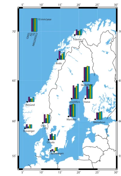
The results in Table 2 show the well-known pattern of high uplift rates at the Gulf of Bothnia (Vaasa, Skellefteå, Kramfors) with gradually falling values towards the edges of the rebound area. The NKG2005LU model shows quite low values for the Norwegian sites compared to the latest GNSS solution. This is most likely due to the fact that in the model the older version of BIFROST solutions (Lidberg et al., 2007) were used and these old values include only Swedish and Finnish sites. The standard deviations for the stations range from 0.6 (Skellefteå) to 1.7 mm yr−1(Onsala and Bodø), indicating more stable land uplift trends on the Baltic Sea, while more variability is seen on the Atlantic coast and Danish straits. The mean of the standard deviations is 1.1 mm yr−1. The values of Table 2 are depicted in Fig. 3.
The contemporary global sea level rise is known to be about 3 mm yr−1 (e.g. Cazenave and Llovel, 2010; Church et al., 2013) which is considerably more than the value used in the NKG2005LU model. The lower value was based on the mean sea level rise in the Baltic Sea in the period 1891– 1990 (Vestøl, 2005). For Table 3, a new value of the sea level rise was computed as a mean of the chosen stations:
˙ He=1
n n
X
i=1 ˙
hi×0.94
5˚ 5˚
10˚ 10˚
15˚ 15˚
20˚ 20˚
25˚ 25˚
30˚ 30˚
55˚ 55˚
60˚ 60˚
65˚ 65˚
70˚ 70˚
Metsahovi Vaasa Skelleftea
Kramfors
Martsbo
Copenhagen Onsala Oslo Stavanger
Alesund
Bodo
Tromso GNSS
AG TG
NKG2005LU 10 mm/year
Figure 3. Land uplift values with the sea level rise estimate of
1.32 mm yr−1(Table 2).
whereH˙eis the mean sea level rise,h˙
iis the absolute land
up-lift value from GNSS,H˙
a,i is the apparent sea level change
from tide gauge data (Table 1) andnis the number of sta-tions. The value 0.94 scales the GNSS-derived uplift value for the 6 % geoid rise (Ekman and Mäkinen, 1996). We ob-tain the value for H˙e=3.11±1.07 mm yr−1, which agrees
with the contemporary sea level rise values from satellite al-timetry (e.g. Cazenave and Llovel, 2010). Table 3 shows the values of land uplift using the value for sea level rise com-puted above. The standard deviations vary from 0.3 to 1.8. The mean of the standard deviations diminishes from 1.1 to 0.99 mm yr−1, which is not surprising, since a mean value computed with this data set was used. The values of Table 3 are depicted in Fig. 4.
A comparison of techniques is challenging since they mea-sure height relative to a different reference level and con-versions are needed to bring all measurements to the same system. Stations with multiple techniques can be used to study the differences and similarities of the measurement techniques, since different techniques are affected by
differ-5˚ 5˚
10˚ 10˚
15˚ 15˚
20˚ 20˚
25˚ 25˚
30˚ 30˚
55˚ 55˚
60˚ 60˚
65˚ 65˚
70˚ 70˚
Metsahovi Vaasa Skelleftea
Kramfors
Martsbo
Copenhagen Onsala Oslo Stavanger
Alesund
Bodo
Tromso GNSS
AG TG
NKG2005LU 10 mm/year
Figure 4. Land uplift values with sea level rise estimate of
3.11 mm yr−1(Table 3).
ent geophysical processes. GNSS observes ellipsoidal height change, whereas a gravimeter observes gravity change due to the height change and redistribution of masses, and tide gauge data are affected by the sea level change and the lo-cal uplift. The GNSS uses the centre of the figure (CF) of Earth (which is at these timescales equivalent to centre of the entire Earth frame (CE)) and is able to observe and moni-tor the Earth’s centre of mass, whereas the absolute gravity measurements are done in the centre of mass frame (CM). Also worth noting is that the z-translation rate of the refer-ence frame has a larger impact on the vertical component at these high latitudes.
is computed for the same period of time that GNSS has been in operation (last 20 years), the values differ markedly from the values of the whole tide gauge record. There might also be large spatial differences, since, e.g. the melt waters from glaciers are not distributed equally on Earth (Tamisiea et al., 2001).
The estimates of global sea level rise for the last century vary between 1 and 1.8 mm yr−1 (Church et al., 2013),
de-pending slightly on the time window. Similar values were obtained for the Baltic Sea (Johansson, et al., 2003) but the question remains whether the same global sea level rise value can be used for the Norwegian coast as for the Baltic. The Baltic Sea is a semi-closed basin where the effect of the North Atlantic Oscillation (NAO) (e.g. Johansson, et al., 2003, 2004) and the effect of the meridional wind (Johansson M. et al., 2012) is noticeable. The strength of prevailing west-erly winds will push less or more water through the Danish straits; thus causing decadal variation of the sea level rise in the Baltic, following the general trend of the NAO index. In general, the Baltic sea follows the sea level rise of the North Sea and North Atlantic, but decadal anomalies can exist as discussed in Johansson et al. (2003).
In the NKG2005LU model, Vestøl (2005) used the value of 1.32 mm yr−1for the sea level rise, which was the best
es-timate for the Baltic Sea in the period 1891–1990 (the value used in Table 2). From satellite altimetry the sea level rise of the last decade is about 3 mm yr−1(Cazenave and Llovel,
2010; Church and White 2011, Johansson et al., 2012). Us-ing the values in Table 1 and Eq. (3) we computed the sea level rise based on the 12 stations in our example. The value of 3 mm yr−1coincides well with the global value given by Cazenave and Llovel (2010). This value is used in Table 3.
The absolute gravity measurements are very sensitive to environmental changes (nearby sea, groundwater, etc.). In many cases, the AG time series may contain only a few obser-vations. Therefore, the difference in the trend estimate from either short or long time series can be significant and any anomalous observation may affect the trend. This can be seen in the case of Onsala and Copenhagen, where changes in the sea level of the Danish straits affect the measurements no-ticeably (Müller et al., 2010; Timmen et al., 2011).
In Table 3 all standard deviations greater than 1 are com-ing from cases where the gravity-based values are deviatcom-ing from the three other techniques. We computed also the case where the AG observations were neglected (last two columns in Table 3). As one can see, the standard deviation diminished significantly, from the mean value of 0.99 to 0.60. More data are needed to make a final conclusion, in general, on the use-fulness and reliability of the AG time series, as the length of the time series used in the present study are only 4 (Breili, 2009) or 5 years (Gitlein, 2010), and the measurements are prone to local effects, as discussed above.
In data processing, problems may also stem from the use of different theoretical models. For example, for both GNSS and gravity computations, the solid Earth tide and ocean tidal
loading are taken into account. Differences in these mod-els’ reference frames have been shown to produce spurious signals in GNSS computation (Fu et al., 2012). Also dif-ferent handling of the solid earth tide in these two specific cases may produce a latitude-dependent bias (Poutanen et al., 1996).
Another theoretical aspect is that the gravity values were transformed using the rate of−0.17 µGal mm−1. This value has been argued in the literature (Wahr et al., 1995; Ekman and Mäkinen, 1996; Mäkinen et al., 2005; Gitlein, 2010). It is a modest approximation, but not necessarily the optimum one. When more gravity data are processed and values also from the subsiding areas are used, the accuracy of the ratio will most likely improve (Mäkinen et al., 2005).
In this study, we have shown that data comparisons are needed to exploit the full potential of the geodetic networks. To fully utilize the potential of different techniques and mea-surements and to avoid problems with different models cho-sen for data handling, all data should be processed for the same time period and using the same models.
One concern with this type of review study is that the user has no control over the observations or data reduction. The authors of the published results have chosen the best observa-tions and models for their study. Thus, the values need to be taken as they are and trust that differences in data selection and processing do not distort the comparison markedly. In order to make comparisons possible and reliable, researchers should document in detail what they have done. Such infor-mation can nowadays be easily embedded into appendixes or other electronically saved background information. Such information should be available in the database.
4 Conclusions
During the last decade, geodesists have proposed and devel-oped regional and global observing systems with several ob-serving techniques at the same site, databases, and combi-nations of different observing techniques. In Nordic coun-tries, the proposed observing system NGOS, organized by the NKG, includes stations in the Nordic countries and Baltic states up to Iceland and Greenland. The first goal of this study was to create a simple database offering access to the network stations and the related data. This was realized by collecting available information and providing an interface with meta-data and relevant links to the users.
compare because they measure different processes and their reference levels are not the same. More work is needed to solve this issue more reliably.
Integrity and reliability are essential when combining multi-technique data; they involve standardized techniques to process the original observations, unified models, and ac-cessible original data and background information. The use of geodetic observing systems is a way to achieve this goal.
The Supplement related to this article is available online at doi:10.5194/se-5-673-2014-supplement.
Special Issue: “Lithosphere-cryosphere interactions”
Edited by: M. Poutanen, B. Vermeersen, V. Klemann, and C. Pascal
References
Ågren, J. and Svensson, R.: Postglacial Land Uplift Model and Sys-tem Definition for the New Swedish Height SysSys-tem RH 2000. LMV-Rapport 2007:4. Reports in Geodesy and Geographical In-formation Systems, Gävle, ISSN 280-5731, 2007.
Breili, K.: Investigations of surface loads of the Earth – geometrical deformations and gravity changes, Ph.D. Thesis, Department of Mathematical Sciences and Technology, Norwegian University of Life Sciences, vol. 2009:25, ISSN 1503-1667, ISBN 978-82-575-0892-0, 2009.
Cazenave, A. and Llovel, W.: Contemporary sea level rise, Annu. Rev. Mar. Sci., 2, 145–173, doi:10.1146/annurev-marine-120308-081105, 2010.
Church, J. and White, N.: Sea-level rise from the late 19th to the early 21st century, Surv. Geophys., 32, 585–602, doi:10.1007/s10712-011-9119-1, ISSN 0169-3298, 2011. Church, J. A., Clark, P. U., Cazenave, A., Gregory, J. M., Jevrejeva,
S., Levermann, A., Merrifield, M. A., Milne, G. A., Nerem, R. S., Nunn, P. D., Payne, A. J., Pfeffer, W. T., Stammer, D., and Un-nikrishnan, A. S.: Sea Level Change, in: Climate Change 2013: The Physical Science Basis. Contribution of Working Group I to the Fifth Assessment Report of the Intergovernmental Panel on Climate Change , edited by: Stocker, T. F., Qin, D., Plattner, G.-K., Tignor, M., Allen, S. G.-K., Boschung, J., Nauels, A., Xia, Y., Bex, V., and Midgley, P. M., Cambridge University Press, Cam-bridge, United Kingdom and New York, NY, USA, 2013. Ekman, M.: A consistent map of the postglacial uplift of
Fennoscan-dia. Terra Nova, 8, 158–165, 1996.
Ekman, M.: Postglacial uplift rates for reducing vertical positions in geodetic reference systems, in: Proceedings of the General Assembly of the Nordic Geodetic Commission, 401–407, ISSN 0280-5731, 1998.
Ekman, M. and Mäkinen, J.: Recent postglacial rebound, gravity change and mantle flow in Fennoscandia, Geophys. J. Int., 126, 229–234, doi:10.1111/j.1365-246X.1996.tb05281.x, 1996. Fu, Y., Freymueller J. T., and van Dam, T.: The effect of using
inconsistent ocean tidal loading models on GPS coordinate so-lutions, J. Geod., 86, 409–421, doi:10.1007/s00190-011-0528-1, 2012.
Gitlein, O.: Absolutgravimetrische Bestimmung der fennoskandis-chen Landhebung mit dem FG5-220, Wissenschaftliche Arbeiten der Fachrichtung Geodäsie und Geoinformatik der Leibniz Uni-versität Hannover, vol. 2009:281, ISSN 0174-1454, ISSN 0065-5325, ISBN 978-3-7696-5055-6, 2010.
Gross, R. and Poutanen, M.: Geodetic Observations of Glacial Iso-static Adjustment. EOS, 90, No. 41, 365, 2009.
Ihde, J., Baker, T., Bruynix, C., Francis, O., Amalvict, M., Keny-eres, A., Mäkinen, J., Shipman, S., Simek, J., and Wilmes, H.: Concept and Status of the ECGN Project, in: EUREF Publica-tion, Symposium Toledo, 4–7 June 2003, in: Mitteilungen des Bundesamtes für Kartographie und Geodäsie, vol. 12:33, Frank-furt a.M., 57–65, 2004.
Johansson, J. M., Davis, J. L., Scherneck, H.-G., Milne, G. A., Vermeer, M., Mitrovica, J. X., Bennett, R. A., Jonsson, B., Elgered, G., Elósegui, P., Koivula, H., Poutanen, M., Rön-näng, B. O., and Shapiro, I. I.: Continuous GPS measure-ments of postglacial adjustment in Fennoscandia. 1. Geode-tic results, J. Geophys. Res.-Sol. Earth, 107, 1978–2012, doi:10.1029/2001JB000400, 2002.
Johansson, M., Kahma, K., and Boman, H.: An improved estimate for the long-term mean sea level on the Finnish coast, Geophys-ica, 39, 51–73, 2003.
Johansson, M., Kahma, K., Boman, H., and Launiainen, J.: Scenar-ios for sea level on the Finnish coast, Boreal Environ. Res., 9, 153–166, 2004.
Johansson, M., Pellikka, H., Kahma K., and Ruosteenoja, K.: Global sea level rise scenarios adapted to the Finnish coast, J. Mar. Syst., 129, 35–46, doi:10.1016/j.jmarsys.2012.08.007, 2012.
Kairus, A.: Pohjoismaisen geodeettisen havaintojärjestelmän käyttö maannousututkimuksessa (using the Nordic Geodetic Observing System for Land Uplift Studies), Master’s thesis, Aalto Univer-sity, 51 pp., 2012 (in Finnish).
Lambeck, K., Smither, C., and Ekman, M.: Test of glacial rebound models for Fennoscandia based on instrumented sea- and lake-level records, Geophys. J. Int., 135, 375–387, 1998.
Lidberg M.: Motions in the Geodetic Reference Frames – GPS ob-servations. Technical Report No. 517, Licentiate Thesis. Depart-ment of Radio and Space Science with Onsala Space Observa-tory, Chamlers University of Technology, Göteborg, 2004. Lidberg, M., Johansson, J. M., Scherneck, H. G., and Davis, J. L.:
An improved and extended GPS-derived 3-D velocity field of the glacial isostatic adjustment (GIA) in Fennoscandia, J. Geod., 81, 213–230. doi:10.1007/s00190-006-0102-4, 2007.
Lidberg, M., Johansson, J. M., Scherneck, H. G., and Milne, G. A.: Recent results based on continuous GPS observations of the GIA process in Fennoscandia from BIFROST, J. Geodyn., 50, 8–18, 2010.
Mäkinen, J., Engfeld, A., Harsson, B. G., Ruotsalainen, H., Strykowski, G., Oja, T., and Wolf, D.: The Fennoscandian land uplift lines 1966–2003, in: Gravity, Geoid and Space Missions GGSM2004, IAG Symposium, vol. 129, Springer, Berlin Hei-delberg, 328–332, 2005.
Pettersen, B.: The postglacial rebound signal of Fennoscandia ob-served by absolute gravimetry, GPS, and tide gauges, Int. J. Geo-phys., 2011, 957329, doi:10.1155/2011/957329, 2011.
Peltier, W. R.: Global glacial isostasy and the surface of the ice-age Earth: the ICE-5G(VM2) model and GRACE, Annu. Rev. Earth Pl. Sc., 32, 111–149, 2004.
Peltier, W. R.: Postglacial variations in the level of the sea: implica-tions for climate dynamics and solid-earth geophysics, Rev. Geo-phys., 36, 603–689, 1998.
Plag, H. P. and Pearlman, M. (Eds.): Global Geodetic Observ-ing System: MeetObserv-ing the Requirements of a Global Society on a Changing Planet in 2020, Springer, doi:10.1007/978-3-642-02687-4, ISBN 978-3-642-02686-7, 2009.
Poutanen, M., Dransch, D., Gregersen, S., Haubrock, E. R. I., Kle-mann, V., Kozlovskaya, E., Kukkonen, I., Lund, B., Lunkka, J. P., Milne, G., Müller, J., Pascal C., Pettersen, B. R., Scher-neck, H. G., Steffen, H., Vermeersen, B., and Wolf, D.: Dy-naQlim – upper mantle dynamics and quaternary climate in cra-tonic areas, in: New Frontiers in Integrated Solid Earth Sciences, edited by: Cloetingh, S. and Negendank, J., Springer, 349–372, doi:10.1007/978-90-481-2737-5_10, 2010.
Poutanen, M., Ihde, J., Bruyninx, C., Francis, O., Kallio, U., Keny-eres, A., Liebsch, G., Mäkinen, J., Shipman, S., Simek, J., Williams, S., and Wilmes, H.: Future and development of the Eu-ropean Combined Geodetic Network ECGN, Earth on the Edge: Science for a Sustainable Planet, Proceedings of the 2011 IAG General Assembly, Melbourne, Australia, edited by: Rizos, C. and Willis, P., International Association of Geodesy Symposia Vol. 139, 121–127, Springer, 2014.
Poutanen, M. and Ivins, E. R.: Upper Mantle Dynamics and Quaternary Climate in Cratonic Areas (DynaQlim) – under-standing the Glacial Isostatic Adjustment, J. Geodyn., 50, 2–7, doi:10.1016/j.jog.2010.01.014, 2010.
Poutanen M., Knudsen, P., Lilje, M., Nørbech, T., Plag, H.-P., and Scherneck, H.-G.: The Nordic Geodetic Observing System (NGOS), in: Dynamic Planet – Monitoring and Understanding a Dynamic Planet with Geodetic and Oceanographic Tools, Con-ference of the International Association of Geodesy, Cairns, Aus-tralia, 22–26 August 2005, vol. 130, edited by: Rizos, C. and Tregoning, P., International Association of Geodesy Symposia, 749–756, 2007.
Poutanen, M., Knudsen, P., Lilje, M., Nørbech, T., Plag, H. P., and Scherneck, H. G.: NGOS – the Nordic Geodetic Observing Sys-tem, Nord. J. Surv. Real Est. Res., 2, 79–100, 2005.
Poutanen M., Vermeer, M., and Mäkinen, J.: The perma-nent tide in GPS positioning, J. Geod., 70, 499–504. doi:10.1007/BF00863622, 1996.
Tamisiea, M., Mitrovica, J., Milne, G. A., and Davis J.: Global geoid and sea level changes due to present-day ice mass fluctuations, J. Geophys. Res.-Sol. Ea., 106, 30849–30864, 2001.
Timmen, L., Gitlein, O., Klemann, V., and Wolf, D.: Observ-ing gravity change in the Fennoscandian uplift area with the Hanover absolute gravimeter, Pure Appl. Geophys., 196, 1331– 1342, doi:10.1007/s00024-011-0397-9, 2011.
van Dam, T., Visser, P., Sneeuw, N., Losch, M., Gruber, T., Bam-ber, J., Bierkens, M., King, M. and Smit, M.: Monitoring and modeling individual sources of mass distribution and transport in the Earth system by means of satellites. Final Report, ESA Contract 20403, 2008.
Vestøl, O.: Determination of postglacial land uplift in Fennoscan-dia from leveling, tide-gauges and continuous GPS sta-tions using least squares collocation, J. Geod., 80, 248–258, doi:10.1007/s00190-006-0063-7, 2005.
Wahr, J. M., Dazhong, H., and Trupin, A.: Predictions of vertical uplift caused by changing polar ice volumes on a viscoelastic Earth, Geophys. Res. Lett., 22, 977–980, 1995.