BGD
9, 18907–18950, 2012
Trait variation in an ESM
L. M. Verheijen et al.
Title Page
Abstract Introduction
Conclusions References
Tables Figures
◭ ◮
◭ ◮
Back Close
Full Screen / Esc
Printer-friendly Version Interactive Discussion
Discussion
P
a
per
|
Dis
cussion
P
a
per
|
Discussion
P
a
per
|
Discussio
n
P
a
per
|
Biogeosciences Discuss., 9, 18907–18950, 2012 www.biogeosciences-discuss.net/9/18907/2012/ doi:10.5194/bgd-9-18907-2012
© Author(s) 2012. CC Attribution 3.0 License.
Biogeosciences Discussions
This discussion paper is/has been under review for the journal Biogeosciences (BG). Please refer to the corresponding final paper in BG if available.
Impacts of trait variation through
observed trait-climate relationships on
performance of a representative Earth
System model: a conceptual analysis
L. M. Verheijen1, V. Brovkin2, R. Aerts1, G. B ¨onisch3, J. H. C. Cornelissen1, J. Kattge3, P. B. Reich4,5, I. J. Wright6, and P. M. van Bodegom1
1
VU University Amsterdam, Systems Ecology, Department of Ecological Science, De Boelelaan 1085, 1081 HV Amsterdam, The Netherlands
2
Max Planck Institute for Meteorology, Bundesstrasse 55, 20146 Hamburg, Germany
3
Max Planck Institute for Biogeochemistry, Hans Knoell Strasse 10, 07745 Jena, Germany
4
University of Minnesota, Department of Forest Resources, 1530 Cleveland Avenue North, St. Paul, MN 55108, USA
5
University of Western Sydney, Hawkesbury Institute for the Environment, Penrith, NSW 2753, Australia
6
BGD
9, 18907–18950, 2012
Trait variation in an ESM
L. M. Verheijen et al.
Title Page
Abstract Introduction
Conclusions References
Tables Figures
◭ ◮
◭ ◮
Back Close
Full Screen / Esc
Printer-friendly Version Interactive Discussion
Discussion
P
a
per
|
Dis
cussion
P
a
per
|
Discussion
P
a
per
|
Discussio
n
P
a
per
|
Received: 12 October 2012 – Accepted: 7 December 2012 – Published: 19 December 2012
Correspondence to: L. M. Verheijen ([email protected])
BGD
9, 18907–18950, 2012
Trait variation in an ESM
L. M. Verheijen et al.
Title Page
Abstract Introduction
Conclusions References
Tables Figures
◭ ◮
◭ ◮
Back Close
Full Screen / Esc
Printer-friendly Version Interactive Discussion
Discussion
P
a
per
|
Dis
cussion
P
a
per
|
Discussion
P
a
per
|
Discussio
n
P
a
per
|
Abstract
In current dynamic global vegetation models (DGVMs), including those incorporated into Earth System Models (ESMs), terrestrial vegetation is represented by a small number of plant functional types (PFTs), each with fixed properties irrespective of their predicted occurrence. This contrasts with natural vegetation, in which many plant
5
traits vary systematically along geographic and environmental gradients. In the JS-BACH DGVM, which is part of the MPI-ESM, we allowed three traits (specific leaf area (SLA), maximum carboxylation rate at 25◦
C (Vcmax25) and maximum electron
trans-port rate (Jmax25)) to vary within PFTs via trait-climate relationships based on a large
trait database. For all three traits, the means of observed natural trait values strongly
10
deviated from values used in the default model, with mean differences of 32.3 % for Vcmax25, 26.8 % for Jmax25 and 17.3 % for SLA. Compared to the default simulation,
allowing trait variation within PFTs resulted in GPP differences up to 50 % in the tropics, in>35 % different dominant vegetation cover, and a closer match with a natural veg-etation map. The discrepancy between default trait values and natural trait variation,
15
combined with the substantial changes in simulated vegetation properties, together emphasize that incorporating observational data based on the ecological concepts of environmental filtering will improve the modeling of vegetation behavior in DGVMs and as such will enable more reliable projections in unknown climates.
1 Introduction
20
Terrestrial vegetation plays a pivotal role in land-atmosphere interactions, modifying carbon, water and heat fluxes via biochemical processes such as photosynthesis and respiration or via biophysical vegetation properties such as stomatal conductance and albedo. Therefore, a correct representation of terrestrial vegetation and its dynamics in Earth System Models (ESMs) is essential, especially for future climate projections. For
25
BGD
9, 18907–18950, 2012
Trait variation in an ESM
L. M. Verheijen et al.
Title Page
Abstract Introduction
Conclusions References
Tables Figures
◭ ◮
◭ ◮
Back Close
Full Screen / Esc
Printer-friendly Version Interactive Discussion
Discussion
P
a
per
|
Dis
cussion
P
a
per
|
Discussion
P
a
per
|
Discussio
n
P
a
per
|
integrate vegetation dynamics with land surface models to allow analysis of transient vegetation responses and feedbacks to climate (Foley et al., 1998; Prentice et al., 2007). Compared to earlier models, vegetation dynamics and interactions between the biosphere and atmosphere have been much improved over the past decade, although many issues still need to be resolved (Quillet et al., 2010).
5
One of these issues is the way in which Plant Functional Types (PFTs) are used to represent vegetation. PFTs are classes of plant species with presumably similar roles in an ecosystem, responding in a comparable manner to environmental conditions like water and nutrient availability (Harrison et al., 2010; Lavorel et al., 1997). They are defined by a combination of attributes such as plant growth form (e.g. trees, shrubs,
10
grasses, herbs), phenology (evergreen, raingreen, summergreen) and bioclimatic tol-erances (e.g. minimum temperature requirements). Notably, most current PFT classi-fications use constant parameter values for some key plant traits, i.e. plant properties that reflect the way plants cope with their environment (McGill et al., 2006; Violle et al., 2007). Using constant plant traits in PFTs has serious limitations (Harrison et al., 2010;
15
Ordo ˜nez et al., 2009; Van Bodegom et al., 2012), as it does not reflect the trait varia-tion observed within and between communities (Ackerly and Cornwell, 2007; Freschet et al., 2011; Kooyman et al., 2010; Westoby et al., 2002), therefore not accounting for local environmental constraints. Furthermore, global trait database analyses have shown that the variation in plant traits is large within PFTs and often even greater than
20
the difference in means among PFTs (Laughlin et al., 2010; Reich et al., 2007; Wright et al., 2005a). Even though PFTs may capture a significant part of the global plant trait variation, a large part (for some traits up to 75 %) may still be unexplained (Kattge et al., 2011) and is thus not represented in current DGVMs.
Given that plants can adjust to the environment via changes in traits, and that such
25
BGD
9, 18907–18950, 2012
Trait variation in an ESM
L. M. Verheijen et al.
Title Page
Abstract Introduction
Conclusions References
Tables Figures
◭ ◮
◭ ◮
Back Close
Full Screen / Esc
Printer-friendly Version Interactive Discussion
Discussion
P
a
per
|
Dis
cussion
P
a
per
|
Discussion
P
a
per
|
Discussio
n
P
a
per
|
models is only possible through shifts in PFT-abundances (Van Bodegom et al., 2012). While in some DGVMs, trait variation has been incorporated to enable modeling of nu-trient cycles (Gerber et al., 2010; Zaehle and Friend, 2010) or was allowed via stochas-tic processes (Alton, 2011), these methods only partly describe the drivers and ranges of the prevailing trait variation.
5
An alternative way to capture and predict trait variation in DGVMs is to include the relationships between natural trait variation and their multiple environmental drivers. At both regional and global scales traits are related to large scale environmental gradients of, for instance, temperature, water and nutrient availability or disturbances (Ordo ˜nez et al., 2009; Van Ommen Kloeke et al., 2012; Wright et al., 2005b). Such
relation-10
ships between environmental conditions and traits can potentially be understood via ecological assembly theory, which describe the processes that determine species as-semblages (Cornwell and Ackerly, 2009; Cornwell et al., 2006; G ¨otzenberger et al., 2012). An important abiotic assembly process is habitat filtering (Keddy, 1992), which describes how local environmental drivers (e.g. soil fertility or precipitation) constrain
15
the range of potential species and related trait values in a given habitat. For many traits, such as specific leaf area, leaf nitrogen and wood density this may contribute to trait convergence within communities (Freschet et al., 2011; Swenson and Enquist, 2007), resulting in global relationships between community trait means and climatic drivers. By identifying the environmental drivers of variation in site trait means, multiple causes
20
of variation are determined and the observed natural trait variation can be modeled with a high level of accuracy.
The aim of this study is thus to improve the modeling of vegetation responses and enable vegetation-atmosphere feedbacks in DGVMs by incorporating climate-driven trait variation within PFTs, based on large observational trait databases. So far
obser-25
BGD
9, 18907–18950, 2012
Trait variation in an ESM
L. M. Verheijen et al.
Title Page
Abstract Introduction
Conclusions References
Tables Figures
◭ ◮
◭ ◮
Back Close
Full Screen / Esc
Printer-friendly Version Interactive Discussion
Discussion
P
a
per
|
Dis
cussion
P
a
per
|
Discussion
P
a
per
|
Discussio
n
P
a
per
|
parameter values per PFT for each individual grid cell, based on a systematic analysis of observed trait-climate relationships.
These relationships were implemented in the JSBACH DGVM, which is part of the Max Planck Institute Earth System Model (MPI-ESM) (Brovkin et al., 2009; Raddatz et al., 2007; Roeckner et al., 2003). It is representative of most DGVMs currently used
5
in the context of ESMs and used in carbon cycle model intercomparisons (Friedling-stein et al., 2006). We simulate variation in three originally constant and PFT-specific key leaf traits in JSBACH: specific leaf area (SLA), maximum carboxylation rate at a ref-erence temperature of 25◦C (Vcmax
25) and maximum electron transport rate at 25◦C
(Jmax25). To determine relationships between these three traits and climatic drivers for
10
each PFT, data from the TRY global plant trait database (Kattge et al., 2011) were re-lated to global climatic data. Based on these relationships between traits and climate, SLA, Vcmax25 and Jmax25were re-parameterized for each grid cell on a yearly basis,
depending on the (local) climatic conditions in a grid cell. This enabled feedbacks be-tween plants and environment, as traits within natural PFTs could vary dynamically in
15
space and time. A simulation with variable traits is compared for trait distribution, pro-ductivity and vegetation distribution to a default simulation with the original trait values of the model, and to an additional simulation with constant, but observation-based, trait values.
As DGVMs are already parameterized to produce approximate realistic results, our
20
variable traits simulation will not necessarily approach reality better than the default simulation. Therefore, in this paper the focus lies on simulation intercomparisons to evaluate the impact of incorporating climate-driven trait variation. A formal validation with observational data is not the primary aim of this paper, as the simulations are not meant to represent current vegetation or climate states, but instead are run into
equilib-25
BGD
9, 18907–18950, 2012
Trait variation in an ESM
L. M. Verheijen et al.
Title Page
Abstract Introduction
Conclusions References
Tables Figures
◭ ◮
◭ ◮
Back Close
Full Screen / Esc
Printer-friendly Version Interactive Discussion
Discussion
P
a
per
|
Dis
cussion
P
a
per
|
Discussion
P
a
per
|
Discussio
n
P
a
per
|
2 Materials and methods
2.1 Model description
Simulations were performed with the ESM of the Max Planck Institute (MPI-ESM). The model setup consisted of the JSBACH DGVM, a land surface model (Raddatz et al., 2007) with a vegetation dynamics module (Brovkin et al., 2009), coupled to the
at-5
mosphere model ECHAM5 (Roeckner et al., 2003) to allow for vegetation-atmosphere feedbacks. The model version on spatial resolution of T63 (approx. 1.875◦, dividing the
world into 18 432 grid cells) with 47 atmospheric layers was used, with atmospheric CO2 concentration kept constant at 353.9 ppm. Seasonal sea surface temperatures and sea ice were prescribed from a default simulation with the MPI ocean model
(MPI-10
OM) (Marsland et al., 2003). Vegetation dynamics were interactive to allow for vege-tation shifts and vegevege-tation-atmosphere feedbacks through trait dynamics. Terrestrial grid cells contained multiple PFTs, each occupying a certain fraction, depending on their competitive ability (based on net primary productivity (NPP)). This study does not include crops and pastures, but focuses on responses of natural vegetation,
repre-15
sented by eight PFTs. These were tropical broadleaved evergreen trees (TrET), trop-ical broadleaved deciduous trees (TrDT), extra-troptrop-ical (both temperate and boreal) evergreen trees (ExTrET), extra-tropical deciduous trees (ExTrDT), raingreen shrubs (RgSh), cold/deciduous shrubs (DSh), C3-grasses (C3G) and C4-grasses (C4G). No anthropogenic land use or land cover change was simulated.
20
2.2 Selected trait and climate data
In JSBACH, SLA (m2kg−1 carbon) is related to the amount of carbon that can be
stored in the green and reserve carbon pools. Vcmax25 (µmol m− 2
s−1
) and Jmax25
(µmol m−2s−1) both control carbon assimilation. Vcmax
25 also determines the
refer-ence respiration at 25◦C. Observational data for these traits (see Table 1 for references)
25
BGD
9, 18907–18950, 2012
Trait variation in an ESM
L. M. Verheijen et al.
Title Page
Abstract Introduction
Conclusions References
Tables Figures
◭ ◮
◭ ◮
Back Close
Full Screen / Esc
Printer-friendly Version Interactive Discussion
Discussion
P
a
per
|
Dis
cussion
P
a
per
|
Discussion
P
a
per
|
Discussio
n
P
a
per
|
for SLA from the database by Van Bodegom et al. (2012) and for Vcmax25 and Jmax25 from Domingues et al. (2010).
Only Vcmax and Jmax standardized to a reference temperature of 25◦C were used.
Most Vcmax and Jmax values had already been standardized to this temperature via the formulation of the photosynthesis model by Farquhar et al. (1980) used in the
con-5
text of JSBACH (Kattge and Knorr, 2007). For other records for which the temperature during measurement was recorded, standardization was done according to this formu-lation. For C4-grasses, variation in PEPcase CO2-specificity (PEP, mmol m−
2
s−1
) in-stead of Jmax25 was determined, following Collatz et al. (1992). Since for C4-grasses
insufficient observational PEP and Vcmax25 data were available, these traits were
es-10
timated more indirectly applying insights from Simioni et al. (2004), who determined PEP and Vcmax25 based on leaf nitrogen (N) content (g m−
2
) (regressions based on two C4-species). Therefore, for C4 grasses, additional information on leaf N was ob-tained from the TRY database.
To link climate and trait data, only geo-referenced trait observations from field
sam-15
pling and field experiments were used. PFT assignment of species was based on avail-able data in the above mentioned databases on growth form (shrub, grass, tree), leaf habit (deciduous/evergreen) and photosynthetic pathway (C3/C4). The climatic domain of a species (tropical, boreal etc.) was determined based on the K ¨oppen-Geiger climate classification (Kottek et al., 2006) and applied to the geo-referenced observations. This
20
resulted in 12 394 observations for SLA distributed over 2869 species and 1052 (PFT-specific) sites, 761 observations over 129 species and 70 sites for Vcmax25 and 402
observations over 108 species and 56 sites for Jmax25 (see supplementary material S1 for global map with locations of trait data).
Global climate data on mean annual precipitation (MAP, mm yr−1), mean annual
rela-25
tive humidity (Reh, %), mean annual temperature (MAT,◦C), mean temperature of
cold-est and warmcold-est month (TminandTmax,◦C) were collected from a global 10 min gridded
BGD
9, 18907–18950, 2012
Trait variation in an ESM
L. M. Verheijen et al.
Title Page
Abstract Introduction
Conclusions References
Tables Figures
◭ ◮
◭ ◮
Back Close
Full Screen / Esc
Printer-friendly Version Interactive Discussion
Discussion
P
a
per
|
Dis
cussion
P
a
per
|
Discussion
P
a
per
|
Discussio
n
P
a
per
|
calculated based on distance to sun and percentage sunshine (from CRU) according to Allen et al. (1998) on a global 30 min spatial resolution. Soil moisture was taken from GLEAM, a methodology that estimates soil moisture and evapotranspiration based on remotely sensed data at a global 15 min spatial resolution (SoilMoist, m3m−3 for 1 m
depth, Miralles et al., 2011). Soil moisture was the only edaphic control of trait variation,
5
since soil N was not modeled in this version of JSBACH.
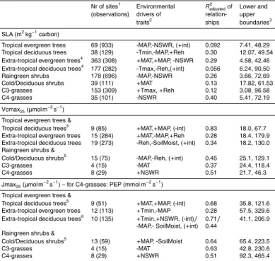
2.3 Trait-climate relationships
Given the lack of global quantitative deterministic predictions, the observed natural variation of SLA, Vcmax25 and Jmax25 was described for each PFT by the simplest
models possible, i.e. linear regressions. For this purpose, we used PFT-specific site
10
means to match the scale of modeled fluxes most closely. Observed site means were related to the multiple environmental conditions at these sites in a linear regression, weighting sites by the square root of the number of observations (data points) per site. Such relationships likely reflect habitat filtering which commonly leads to trait conver-gence at community scales. Regressions with the highest explained variance (highest
15
Radjusted2 ) were selected, after checking for significance of climatic drivers and distri-bution of residuals. In case of co-linearity between environmental drivers (Pearson’s correlation higher than 0.7 or lower than−0.7), the driver with lowest significance was omitted. Due to the low number of sites for Vcmax25and Jmax25, data for the two
trop-ical tree PFTs were combined, as well as data for the two shrub PFTs. This resulted in
20
eight relationships for SLA and six for both Vcmax25 and Jmax25. These relationships were subsequently implemented in JSBACH. In addition, to allow trait calculations to go beyond climatic regions used in the regressions, but to still maintain traits within ranges as observed in nature, simulated trait ranges were constrained to the 2.5–97.5% quan-tiles of all individual observations within a PFT (instead of the site means). For Jmax25
25
and Vcmax25,an additional constraint was applied to maintain the strong physiological
BGD
9, 18907–18950, 2012
Trait variation in an ESM
L. M. Verheijen et al.
Title Page
Abstract Introduction
Conclusions References
Tables Figures
◭ ◮
◭ ◮
Back Close
Full Screen / Esc
Printer-friendly Version Interactive Discussion
Discussion
P
a
per
|
Dis
cussion
P
a
per
|
Discussion
P
a
per
|
Discussio
n
P
a
per
|
these two traits (as determined per PFT). Predicted values outside this range were ad-justed to the confidence interval border, based on the shortest distance needed to reach the border. Since this version of JSBACH did not simulate N-cycling, soil N could not be used to parameterize Vcmax25, even though N-availability is a strong
determi-nant (see references in Kattge et al., 2009). However, the above two constraints on
5
Vcmax25were based on observational data, indirectly incorporating N-limitations.
2.4 Simulation setups
Three different scenarios were performed: 1. a simulation containing the default pa-rameterization of JSBACH with constant parameter values per PFT, based on Raddatz et al. (2007) and Kattge et al. (2009), and adapted to approximate realistic
vegeta-10
tion functioning within the vegetation dynamics module (Brovkin et al., 2009); hereafter called “default simulation”, 2. an “observed traits simulation” again with constant val-ues for SLA, Vcmax25 and Jmax25 per PFT, but based on observational data only (the
weighted site means for each PFT, from here on called “observed global means”), and 3. a “variable traits simulation” in which traits were allowed to vary depending on local
15
climatic conditions. In the latter simulation, at the beginning of every year each of the three key traits was re-parameterized for each PFT in every terrestrial grid cell of the world, depending on the local simulated climatic conditions in each grid cell. The ob-served traits simulation was performed in order to separate the effects of replacing trait constants by observations from the effects of trait variation in the model.
20
To get vegetation into quasi-equilibrium with the simulated climate (but with CO2 con-centration fixed), the coupled model (JSBACH/ECHAM5) was run for 150 yr with vege-tation dynamics in an accelerated mode (i.e. vegevege-tation was simulated 3 times for each year of simulated climate). Next, to get the slow soil carbon pools into equilibrium, the uncoupled carbon model of JSBACH (“CBALANCE”) was run for 1500 yr. The coupled
25
BGD
9, 18907–18950, 2012
Trait variation in an ESM
L. M. Verheijen et al.
Title Page
Abstract Introduction
Conclusions References
Tables Figures
◭ ◮
◭ ◮
Back Close
Full Screen / Esc
Printer-friendly Version Interactive Discussion
Discussion
P
a
per
|
Dis
cussion
P
a
per
|
Discussion
P
a
per
|
Discussio
n
P
a
per
|
which in this setup (with prescribed seasonal sea surface temperatures) was sufficient to account for the inter-annual climate variation.
2.5 Data comparison
Model performance was investigated by comparing vegetation distribution, GPP and biomass of the simulations with observations. Vegetation distribution of the dominant
5
PFT (Fig. 5) was compared to the potential (natural) vegetation map of Ramankutty and Foley (1999), which in part is used to initialize simulations in JSBACH. The mismatch in spatial resolution (the potential vegetation maps is at a global 30 min spatial resolution) was solved by counting the number of PFTs according to Ramankutty and Foley (1999) that were present in each JSBACH-grid cell. The PFT with the highest occurrence was
10
compared with the simulated dominant PFT of JSBACH.
To match the PFT-classifications, aggregated PFTs were constructed (Table S4.1, Fig. S4.1), as the PFTs of Ramankutty and Foley (1999) could not be directly related to those of JSBACH. Temperate and boreal evergreen trees were merged to match extra-tropical evergreen trees in JSBACH. The same was done for deciduous trees. Shrubs
15
(marginal in JSBACH) were merged into a single PFT (“shrubs”) in both JSBACH and the vegetation map. As savannas consist of grasslands and woodlands, matches be-tween savannas and C4-grasses or tropical broadleaved deciduous trees were both classified as correct. Tundra and mixed forests were omitted from the comparison as no equivalent PFT was available in JSBACH.
20
Model performance was determined with Cohen’s kappa (κ) (Cohen, 1960), which is the proportion of agreement between vegetation maps, while accounting for chance agreement. Grid cells with sea or ice as the dominant cover were not taken into ac-count, and neither were cases in which more than 1 PFT shared the highest occurrence (i.e. equal number of grid cells). This resulted in a comparison of 2819 grid cells.
25
BGD
9, 18907–18950, 2012
Trait variation in an ESM
L. M. Verheijen et al.
Title Page
Abstract Introduction
Conclusions References
Tables Figures
◭ ◮
◭ ◮
Back Close
Full Screen / Esc
Printer-friendly Version Interactive Discussion
Discussion
P
a
per
|
Dis
cussion
P
a
per
|
Discussion
P
a
per
|
Discussio
n
P
a
per
|
including land use change and crops, comparing global total biomass would result in an overestimation by our simulations. Therefore, comparisons were made per m2 per (aggregated) PFT.
JSBACH does not have a separate savanna-like PFT. Therefore, tropical forests and C4-grasslands were averaged and compared with averages of tropical forests and
sa-5
vanna. Furthermore, extra-tropical trees were averaged and compared with averaged temperate and boreal trees of Robinson (2007). Mediterranean shrubs and tundra were omitted as there were no comparable PFTs in JSBACH.
Latitudinal patterns of median GPP were compared with data taken from Beer et al. (2010), who combined observational data (eddy covariance fluxes) with diagnostic
10
models to approximate GPP.
3 Results
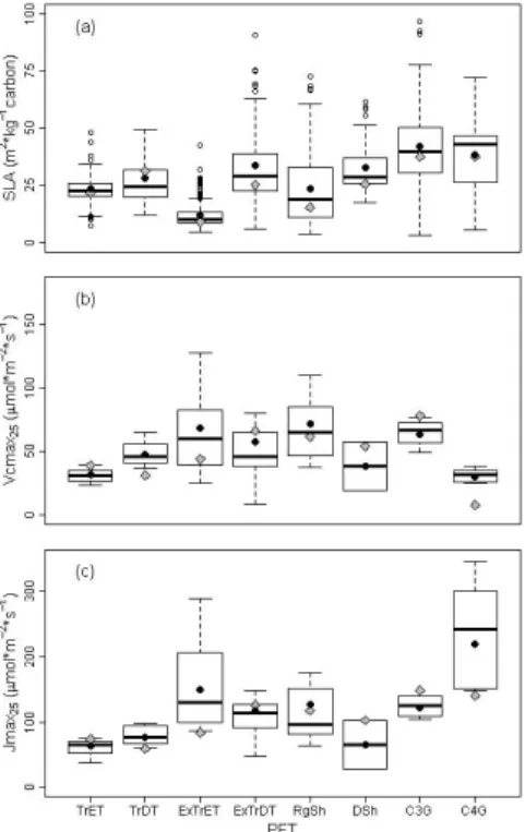
3.1 Mismatch between observed trait data and default trait settings
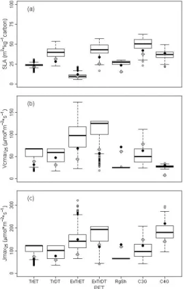
Within each PFT, a large observed range in the three trait values was apparent, as well as large overlap in trait ranges among PFTs (Fig. 1). This was most manifest for
15
SLA, where all PFTs overlapped with each other. For Vcmax25, the only PFTs of which the 95 % confidence interval did not overlap were both tropical evergreen trees and C4-grasses with C3-grasses and for Jmax25 both tropical trees and deciduous shrubs
with C3-grasses.
For all three traits, the default parameter values deviated strongly from the
PFT-20
specific observed global means (grey diamonds and black circles in Fig. 1) in the ob-served traits simulation. Differences between these default traits and observed global means of PFTs were on average 32.3 % for Vcmax25, 26.8 % for Jmax25and 17.3 % for
SLA (but for specific PFTs going up to 73.4 %, 57.6 % and 35.2 %, respectively). Kattge et al. (2011) already showed that often PFT-specific constant SLA values in DGVMs
25
BGD
9, 18907–18950, 2012
Trait variation in an ESM
L. M. Verheijen et al.
Title Page
Abstract Introduction
Conclusions References
Tables Figures
◭ ◮
◭ ◮
Back Close
Full Screen / Esc
Printer-friendly Version Interactive Discussion
Discussion
P
a
per
|
Dis
cussion
P
a
per
|
Discussion
P
a
per
|
Discussio
n
P
a
per
|
the observed data distribution. In JSBACH, SLA default values were always lower than the observed global means, except for the tropical broadleaved deciduous trees, but they almost all fell within the 25 % quartiles of the observed range of SLA, except for deciduous shrubs. However, for both Vmax25and Jmax25default values fell outside the 25 % quartiles for more than half of the PFTs (five out of eight PFTs for both), and even
5
outside the minimum and maximum values of observed trait ranges in some cases (tropical deciduous trees, C4-grasses and C3-grasses for Vcmax25 and Jmax25, and additionally extra-tropical evergreen trees for Jmax25). In contrast to SLA, there was no
clear direction of the trait differences for either Vcmax25 or Jmax25: half of the default
values were lower than the observed global means (Tropical Deciduous Trees,
Extra-10
tropical Evergreen Trees, Raingreen shrubs and C4-grasses), the other half higher. These differences point to a strong mismatch between default trait-parameters in JS-BACH with observed natural trait means.
3.2 Simulated trait variation based on climatic drivers
The observed variation in PFT-specific site means was related to variation in
environ-15
mental drivers (Table 2). All regressions were significant, except for C3-grasses for Vmax25 and for Jmax25. Although the selected environmental drivers (Table 2) differed
among PFTs, net shortwave radiation (NSWR) and mean annual precipitation (MAP) were most frequently selected as drivers for SLA, as were MAP, mean annual tem-perature (MAT) and relative humidity (Reh) for Vcmax25and MAP for Jmax25.R
2 adjusted
20
was up to 0.83 for Vcmax25 and 0.71 for Jmax25. For SLA, more variation remained
unexplained, with a maximum value of 0.40 forRadjusted2 .
Figure 2 presents the trait ranges of the dominant PFT in every grid cell in the variable traits simulation as predicted by the trait-climate relationships. For each grid cell, only trait values of the dominant PFTs are selected to prevent trait values of marginal PFTs
25
BGD
9, 18907–18950, 2012
Trait variation in an ESM
L. M. Verheijen et al.
Title Page
Abstract Introduction
Conclusions References
Tables Figures
◭ ◮
◭ ◮
Back Close
Full Screen / Esc
Printer-friendly Version Interactive Discussion
Discussion
P
a
per
|
Dis
cussion
P
a
per
|
Discussion
P
a
per
|
Discussio
n
P
a
per
|
PFTs had one constant value per trait, a large climate-driven trait range was predicted for the variable traits simulation. The higher SLA of deciduous versus evergreen trees observed in natural vegetation was reflected in the simulated SLA ranges. As for the observations, there was large overlap in trait ranges among PFTs for the three simu-lated traits as well, particularly for Vcmax25 and Jmax25. Simulated SLA-ranges were
5
narrower and overlapped less among PFTs compared to observed ranges (Fig. 1). For all three traits, a strong mismatch of default traits with the simulated trait variation was apparent again: for SLA default values fell (at least) outside the 25–75 % inter-quartile range in four PFTs (vs. one in the observed data), and for Vcmax25 and Jmax25 for
every PFT.
10
3.3 Inclusion of trait variation alters predicted global patterns of productivity
The observed traits and variable traits simulation showed a similar pattern of median GPP along the latitudinal gradient compared to the default simulation (Fig. 3), but in ab-solute values GPP was much higher in the variable traits simulation in the geographic zone between about 30◦S and 30◦N (
∼50 % around the equator and twice as much
15
between 25–30◦
N). GPP of the observed traits simulation also reached higher values (up to twice as much) as the default between 25–30◦N, but had lower values than the
variable traits simulation between−20◦S and 15◦N, and highest values (64–67 %) at
higher latitudes. NPP differences between about 30◦
S and 30◦
N were less profound than for GPP, showing that trait variation affects global patterns of GPP and NPP in
20
different ways. Again, at higher latitudes, the observed traits simulation predicted high-est NPP. For the variable traits simulation, the reduction from gross to net primary productivity around the tropics is much stronger than for either other simulation, re-sulting in smaller NPP differences among simulations compared to GPP differences (even though differences may still go up to 75 % between 25–30◦
N for both observed
25
BGD
9, 18907–18950, 2012
Trait variation in an ESM
L. M. Verheijen et al.
Title Page
Abstract Introduction
Conclusions References
Tables Figures
◭ ◮
◭ ◮
Back Close
Full Screen / Esc
Printer-friendly Version Interactive Discussion
Discussion
P
a
per
|
Dis
cussion
P
a
per
|
Discussion
P
a
per
|
Discussio
n
P
a
per
|
exceeding the maximum sizes of the different carbon pools (e.g. of leaves, wood, re-serves) as defined in JSBACH, resulting in respiration of excess carbon. This loss of excess carbon is visible in the tropical regions for all simulations, but for the variable traits simulation this resulted in a proportionally larger amount of productivity removed. This was enhanced by the higher SLA in these regions, which partly determines the
5
amount of carbon stored in the living parts of the plants, consisting of leaves, fine roots and sapwood.
These results show that, while reproducing global patterns of productivity, incorporat-ing global trait variation in the model leads to strong changes in predicted productivity. Even though GPP is not only determined by the photosynthetic parameters (Vcmax25
10
and Jmax25), as it is affected by e.g. water availability as well, on average, shifts in GPP were accompanied by shifts in similar directions by mean Vcmax25 and Jmax25
(weighted by fractional coverage of PFTs), compared to the default simulation (Fig. 4). However, this was not always the case, as e.g. the drop in Vcmax25and Jmax25above 40◦
N did not lead to a coinciding drop in GPP. Productivity could not be related to
15
similar shifts in SLA.
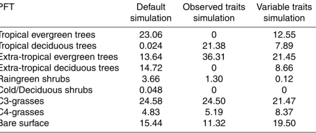
3.4 Major shifts in vegetation distribution
Figure 5 and Table 3 show how the global distribution of dominant vegetation types as predicted by the simulations strongly changes when incorporating observed global trait values or including trait variation based on observation-based trait-climate
rela-20
tionships. A PFT was considered dominant if it had the highest fractional coverage in a grid cell; this ranged from coverage of almost 100 % (mostly in tropical regions) to only 30 % in some areas at higher latitudes (see S2 for fractional coverage of the dom-inant PFTs). Predicted domdom-inant PFTs differed from the default simulation in 35.4 % of the terrestrial grid cells for the variable traits simulation and in 50.5 % of the grid cells
25
for the observed traits simulation.
BGD
9, 18907–18950, 2012
Trait variation in an ESM
L. M. Verheijen et al.
Title Page
Abstract Introduction
Conclusions References
Tables Figures
◭ ◮
◭ ◮
Back Close
Full Screen / Esc
Printer-friendly Version Interactive Discussion
Discussion
P
a
per
|
Dis
cussion
P
a
per
|
Discussion
P
a
per
|
Discussio
n
P
a
per
|
and extra-tropical deciduous trees were replaced by extra-tropical evergreen trees as the dominant PFT, resulting in less spatially heterogeneous dominant vegetation. In the variable traits simulation these shifts occurred as well (see Fig. 5 and Table 3). How-ever, in contrast to the observed traits simulation, both changes in dominant tree cover only occurred in limited areas, which resulted in more spatial variation in vegetation in
5
the areas where trees were dominant. The shifts from tropical evergreen to tropical de-ciduous trees cannot be explained by Vcmax25and Jmax25, since these tropical PFTs
were parameterized with the same values for these traits. The most profound diff er-ence between these tropical PFTs seems to be their leaf turnover rate, which is higher for the deciduous than for the evergreen trees. As a consequence, tropical
decidu-10
ous trees had somewhat lower leaf area index (LAI), which meant lower productivity in favorable periods, but also less carbon loss in more stressful circumstances (e.g. drier periods). In some areas, this could have resulted in a higher total yearly NPP for tropical deciduous trees, thereby outcompeting evergreen trees.
Another shift in predicted dominant vegetation in the variable traits simulation was
15
an increase in C4-grasses (from 4.8 % in the default simulation to 8.4 %). This oc-curred mostly in Africa and Australia at the expense of tropical trees and raingreen shrubs. This expansion of C4-grasses below the Sahara coincided with higher frac-tions of burned area, which promoted the expansion of grasses at the cost of trees.
In the variable traits simulation bare ground increased as dominant cover type (from
20
15.4 in the default simulation to 19.5 %) in the southwest of the United States (and Mexico), northern Canada and northeast of Siberia at the expense of C3-grasses and deciduous trees, resulting in a shift of the boreal tree-line toward lower latitudes. These shifts often coincided with a decrease in Vcmax25 (see S3), suggesting lower produc-tivity and consequently less expansion of these PFTs.
25
3.5 Modulation of climate by traits
BGD
9, 18907–18950, 2012
Trait variation in an ESM
L. M. Verheijen et al.
Title Page
Abstract Introduction
Conclusions References
Tables Figures
◭ ◮
◭ ◮
Back Close
Full Screen / Esc
Printer-friendly Version Interactive Discussion
Discussion
P
a
per
|
Dis
cussion
P
a
per
|
Discussion
P
a
per
|
Discussio
n
P
a
per
|
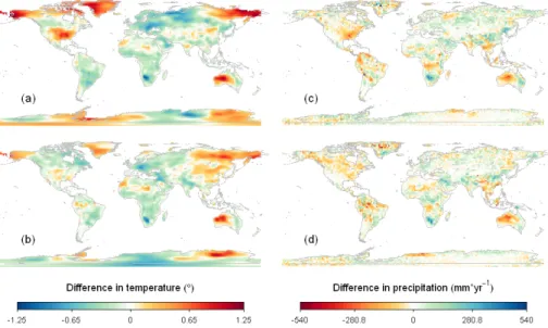
(Fig. 6c, d), but in the variable traits and observed traits simulations it was drier in Canada, Asia and Australia, as well as in large parts of the Amazon rainforests com-pared to the default simulation.
Compared to the default simulation, in the observed traits simulation mean annual surface-air temperatures were profoundly higher (over 1◦C) in Eastern Siberia, Alaska,
5
the US and Australia, and lower (up to 1◦C) in large parts of Europe and Russia,
South-Africa and South-America (Fig. 6a), meaning that (at least) temperature is very sensitive to parameterization of traits.
Temperature differences were less profound between default and the variable traits simulation (Fig. 6b), but still went up to around 1◦C. Changes in temperature did not
10
correlate with clear changes in traits or vegetation shifts (e.g. tree-grass shifts), but in the Southern Hemisphere (Australia, Africa, South-America) corresponded to dif-ferences in transpiration, where cooler areas coincided with higher transpiration. This could be related to the higher Vcmax25 in these areas, resulting in higher GPP and consequently an increase in transpiration.
15
The differences between the observed traits simulation and variable traits simulation indicate that by allowing traits to vary and respond to environmental conditions (as in the variable traits simulation) feedbacks between climate and traits result in more moderate temperature shifts, showing the significant magnitude of adaptive traits and on climate.
20
3.6 Comparison of model output with observational data
Cohen’sκ, indicating the correspondence of the global map of potential (natural) veg-etation of Ramankutty and Foley (1999) with simulated vegveg-etation distribution, was 0.289, 0.282 and 0.334 for the default, observed traits and variable traits simulation, respectively. These values are somewhat lower than the performance of other DGVMs
25
BGD
9, 18907–18950, 2012
Trait variation in an ESM
L. M. Verheijen et al.
Title Page
Abstract Introduction
Conclusions References
Tables Figures
◭ ◮
◭ ◮
Back Close
Full Screen / Esc
Printer-friendly Version Interactive Discussion
Discussion
P
a
per
|
Dis
cussion
P
a
per
|
Discussion
P
a
per
|
Discussio
n
P
a
per
|
there is a substantial increase in similarity to observed vegetation from the default and observed traits simulation toward the variable traits simulation.
Mismatches occurred in large parts of the US and Canada, where the simulations predicted mostly C3-grasslands, while according to the potential vegetation map also forests should be present. The same holds for large parts of Europe. The potential
5
vegetation map shows less bare ground than any simulation, resulting in mismatches in the US, but also other parts of the world. Furthermore, almost the whole continent of Australia did not correspond to this map; shrubs and savanna are dominant according to the map, and even though the models did predict C4-grasses there, it was in diff er-ent areas. Where the default and observed traits simulation had low correspondence
10
with the vegetation map in Africa and South-America, the variable traits simulation performed better, mainly with respect to the tropical trees. Even though differences in performance are small, the variable traits simulation matched the potential vegetation map most closely.
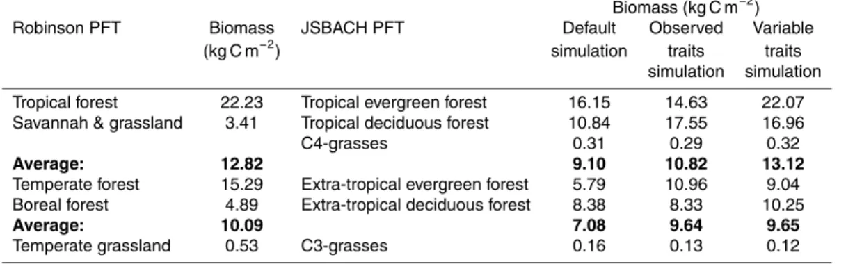
Comparisons of biomass estimates per m2 per (aggregated) PFT with current
15
biomass estimates by Robinson (2007), show that for the combined tropical trees and savannas the variable traits simulation (13.12 kg C m−2) most closely matched biomass
estimates (12.82 kg C m−2
) (Table 4). For extra-tropical (temperate and boreal) forest and temperate grasslands, the default simulation underestimates carbon in vegetation, but both the observed traits and variable traits simulation (9.64 and 9.65 kg C m−2) are
20
close to the global estimates for forests (10.09 kg C m−2
). For temperate grasslands, ei-ther simulation underestimates biomass, with the default simulation deviation the least from global estimates (0.16 vs. 0.53 kg C m−2), even though di
fferences between sim-ulations are small. Overall, this implies that of the three simsim-ulations, the variable traits simulation gives the best global biomass estimates per PFT per m2.
25
BGD
9, 18907–18950, 2012
Trait variation in an ESM
L. M. Verheijen et al.
Title Page
Abstract Introduction
Conclusions References
Tables Figures
◭ ◮
◭ ◮
Back Close
Full Screen / Esc
Printer-friendly Version Interactive Discussion
Discussion
P
a
per
|
Dis
cussion
P
a
per
|
Discussion
P
a
per
|
Discussio
n
P
a
per
|
having the smallest differences. However, Chen et al. (2012) suggest that global GPP estimates based on remotely sensed LAI is underestimated by 9 % when leaf clumping is not taken into account, as this would result in an underestimation of the contribution of shaded leaves to GPP, with the strongest underestimation occurring in the tropics. This implies that the estimates of GPP by Beer et al. (2010) may be too low and thus the
5
actual differences may be less. Also many other DGVMs show higher GPP in the tropi-cal areas than the observed median GPP by Beer et al. (2010) and the GPP estimates of the variable traits simulation still do fall within the upper range of GPP predictions by other DGVMs.
4 Discussion
10
The aim of this study was to improve modeling of vegetation responses and al-low vegetation-atmosphere feedbacks in DGVMs by incorporating trait variation. This trait variation was based on relationships between measured traits and climate and soil moisture, representing major assembly processes by the abiotic environment. As model intercomparisons have shown that large uncertainties exist in projections of land
15
carbon uptake by DGVMs (Cramer et al., 2001; Friedlingstein et al., 2006), incorpo-ration of variation in vegetation responses is important to allow feedbacks between vegetation and climate and to increase plausibility of model predictions, especially un-der strong climate change. Here, we incorporated variation in plant responses based on observed trait and climate data into the JSBACH DGVM, which revealed profound
20
effects on carbon fluxes and vegetation distribution.
4.1 Advantages of modeling trait variation based on trait-climate relationships
We used trait-climate relationships to describe the observed natural trait variation and implemented these in JSBACH. The use of such relationships is broadly accepted and applied in ecology (Ordo ˜nez et al., 2010; Wright et al., 2005b) and identifies and
BGD
9, 18907–18950, 2012
Trait variation in an ESM
L. M. Verheijen et al.
Title Page
Abstract Introduction
Conclusions References
Tables Figures
◭ ◮
◭ ◮
Back Close
Full Screen / Esc
Printer-friendly Version Interactive Discussion
Discussion
P
a
per
|
Dis
cussion
P
a
per
|
Discussion
P
a
per
|
Discussio
n
P
a
per
|
captures multiple (approximate) drivers of natural trait variation. The relationships are thought to reflect abiotic assembly processes and integrate multiple vegetation re-sponses at different temporal and spatial scales, including acclimation, adaptation of species and species replacement into a spatially and temporally varying trait mean. Re-cently, other DGVMs implemented some trait variation necessary to allow feedbacks
5
when modeling N-cycles (Gerber et al., 2010; Zaehle and Friend, 2010). However, in these models effects of trait variation on vegetation cannot be separated from nutrient effects, whereas our study focuses on direct effects of trait variation. Furthermore, the drivers of trait variation in those studies are limited and mainly based on soil N (indi-rectly included in our study through variation in Vcmax25), whereas here multiple drivers
10
of variation have been identified, including water availability (Misson et al., 2006). Even though our proposed method does not explain mechanistically the processes behind trait variation and does not take into account effects of biotic interactions or dispersal on trait values (similar to most DGVMs), it is in our opinion an important and necessary step as it reflects the observed causality between traits and climatic drivers (Niinemets,
15
2001; St. Paul et al., 2012; Wright et al., 2005b). It has the advantage that it does iden-tify and quaniden-tify multiple abiotic drivers of trait means and in this way captures a large part of observed trait variation, as shown by the substantial Radjusted2 of most regres-sions.
We updated trait values once per year. This time-step is a balance between
com-20
putational efficiency and ecological realism. By this approach we avoid to evaluate ontogenic impacts on trait values and whether environmental impacts differ for different parts of the growing season, for which currently insufficient information is available. Our approach assumes that the yearly updated leaf trait values are in equilibrium with their environments, which is consistent with ecological observations. Compared to e.g. wood
25
BGD
9, 18907–18950, 2012
Trait variation in an ESM
L. M. Verheijen et al.
Title Page
Abstract Introduction
Conclusions References
Tables Figures
◭ ◮
◭ ◮
Back Close
Full Screen / Esc
Printer-friendly Version Interactive Discussion
Discussion
P
a
per
|
Dis
cussion
P
a
per
|
Discussion
P
a
per
|
Discussio
n
P
a
per
|
three years in the model, so shifts occur for at least a third of the leaves for these trees. Moreover, the yearly shift in leaf trait values may not only reflect acclimation, but genetic adaptation and species replacements may also contribute. In our approach, in contrast to a mechanistic approach, the impacts and (unknown) time-scales of those processes leading to trait shifts do not have to be differentiated.
5
4.2 Implications of incorporating observation-based trait variation
The observed global mean trait values of natural vegetation as used in the observed traits simulation strongly deviated from trait values in the default simulation, indicat-ing a mismatch between PFT trait means of modeled and natural vegetation. More-over, either set of constant values contrasts strongly with the large range of trait
val-10
ues observed in natural vegetation (Fig. 1). While we applied the most comprehen-sive database available today, we are aware that estimates of observed trait variation are still uncertain (Table 2) and need to be improved in future applications. Neverthe-less, the wide range of observed trait values illustrates how simulations with constant traits do not reflect natural trait variation. In contrast, this variation was reflected by the
15
variable traits simulation where trait variation represented abiotic assembly processes (Fig. 2).
To investigate the effects of trait variation on vegetation-climate feedbacks it was es-sential to incorporate vegetation dynamics, to allow trait shifts to alter vegetation distri-bution and in this way modulate productivity and climate. In contrast to the simulations
20
with constant traits, the variable traits simulation enabled such interactions between vegetation and climate via traits to occur. These interactions resulted in more spa-tial variation in dominant vegetation compared to the other two simulations. As such, predicted vegetation distribution is more a result of temporal dynamics in vegetation properties than is the case in the other simulations, where these vegetation
proper-25
BGD
9, 18907–18950, 2012
Trait variation in an ESM
L. M. Verheijen et al.
Title Page
Abstract Introduction
Conclusions References
Tables Figures
◭ ◮
◭ ◮
Back Close
Full Screen / Esc
Printer-friendly Version Interactive Discussion
Discussion
P
a
per
|
Dis
cussion
P
a
per
|
Discussion
P
a
per
|
Discussio
n
P
a
per
|
directly modulated model output. This problem is well known (Quillet et al., 2010) and stresses the importance of simulations like the ones presented.
Provided the strong effect exerted by climate on traits, major differences among the simulations in predicted vegetation distribution and productivity were expected, the lat-ter especially when paramelat-ters that affect assimilation rate are concerned, as
sensitiv-5
ity analyses of DGVMs have shown (White et al., 2000; Zaehle et al., 2005). Indeed, for the observed traits simulation and variable traits simulation this resulted in large dif-ferences in the new equilibrium state, both compared to the default and to each other. Not only were vegetation properties affected, but also climate changed and mean tem-peratures were altered by up to more than 1◦C.
10
As the simulations in this study provide equilibrium states, and as such do not nec-essarily correspond to current climate or vegetation composition, model comparison to observational data must be interpreted with care, although it does provide insights in the realism of the simulations. DGVMs are parameterized to produce approximately realistic results, and therefore our simulations were not expected to approach
obser-15
vations better than the default simulation. Even though the variable traits simulations produced high GPP for tropical areas, its biomass estimates and vegetation distribution more closely resembled observational data than the default simulation.
The large differences in model output, the mismatch between default trait values in the model and observed trait variation in nature, and the improved performance of the
20
variable traits simulation, demonstrate that – besides a correct representation of plant physiology (e.g. photosynthesis, transpiration) – integration of ecological theory will help to improve vegetation representation in DGVMs and ESMs. Allowing for variable vegetation responses to climate and enabling plant-atmosphere feedbacks will have im-portant consequences for predictions by vegetation models, for vegetation distribution
25
and productivity as well as for global current and future climate. A model intercompar-ison with this approach under elevated CO2 projections, for which large uncertainties
BGD
9, 18907–18950, 2012
Trait variation in an ESM
L. M. Verheijen et al.
Title Page
Abstract Introduction
Conclusions References
Tables Figures
◭ ◮
◭ ◮
Back Close
Full Screen / Esc
Printer-friendly Version Interactive Discussion
Discussion
P
a
per
|
Dis
cussion
P
a
per
|
Discussion
P
a
per
|
Discussio
n
P
a
per
|
5 Conclusions
In this study, we have shown how the ecological representation of vegetation responses and vegetation-atmosphere feedbacks in DGVMs can be improved by incorporation of trait variation via trait-climate relationships. The current mismatch of constant trait values in DGVMs with observed natural trait variation and the impact of incorporation of
5
trait variation on model behavior with respect to vegetation distribution, productivity and global climate, together emphasize the need for implementation of more observation-based trait variation and concomitant ecological concepts. The suggested approach, based on such data and concepts, reflects vegetation acclimation and adaptation to the environment, and will enable more reliable modeling of vegetation behavior under
10
unknown climates.
Supplementary material related to this article is available online at: http://www.biogeosciences-discuss.net/9/18907/2012/
bgd-9-18907-2012-supplement.pdf.
Acknowledgement. This study has been financed by the Netherlands Organisation for
Scien-15
tific Research (NWO), Theme Sustainable Earth Research (project number TKS09-03). Fur-thermore, this study was supported by the TRY initiative on plant traits (http://www.try-db.org). TRY hosted, developed and maintained TRY is hosted, developed and maintained by J. Kattge and G. B ¨onisch (Max Planck Institute for Biogeochemistry, Jena, Germany) and is supported by DIVERSITAS, IGBP, the Global Land Project, QUEST and GIS “Climat, Environnement et
20
BGD
9, 18907–18950, 2012
Trait variation in an ESM
L. M. Verheijen et al.
Title Page
Abstract Introduction
Conclusions References
Tables Figures
◭ ◮
◭ ◮
Back Close
Full Screen / Esc
Printer-friendly Version Interactive Discussion
Discussion
P
a
per
|
Dis
cussion
P
a
per
|
Discussion
P
a
per
|
Discussio
n
P
a
per
|
References
Ackerly, D. D. and Cornwell, W. K.: A trait-based approach to community assembly: partitioning of species trait values into within- and among-community components, Ecol. Lett., 10, 135– 145, doi:10.1111/j.1461-0248.2006.01006.x, 2007.
Allen, R. G., Pereira, L. S., Raes, D., and Smith, M.: Crop evapotranspiration – Guidelines
5
for computing crop water requirements, FAO Irrigation and drainage paper 56, Food and Agriculture Organization of the United Nations, Rome, 1998.
Alton, P. B.: How useful are plant functional types in global simulations of the carbon, water, and energy cycles?, J. Geophys. Res.-Biogeo., 116, G01030, doi:10.1029/2010JG001430, 2011.
10
Bahn, M., Wohlfahrt, G., and Haubner, E.: Leaf photosynthesis, nitrogen contents and specific leaf area of 30 grassland species in differently managed mountain ecosystems in the Eastern Alps, in: Land-Use Changes in European Mountain Ecosystems. ECOMONT – Concepts and Results, edited by: Cernusca, A., Tappeiner, U., and Bayfield, N., Blackwell, Wissenschaft, Berlin, 247–255, 1999.
15
Beer, C., Reichstein, M., Tomelleri, E., Ciais, P., Jung, M., Carvalhais, N., Roedenbeck, C., Arain, M. A., Baldocchi, D., Bonan, G. B., Bondeau, A., Cescatti, A., Lasslop, G., Lin-droth, A., Lomas, M., Luyssaert, S., Margolis, H., Oleson, K. W., Roupsard, O., Veenen-daal, E., Viovy, N., Williams, C., Woodward, F. I., and Papale, D.: Terrestrial gross car-bon dioxide uptake: global distribution and covariation with climate, Science, 329, 834–838,
20
doi:10.1126/science.1184984, 2010.
Brovkin, V., Raddatz, T., Reick, C. H., Claussen, M., and Gayler, V.: Global biogeo-physical interactions between forest and climate, Geophys. Res. Lett., 36, L07405, doi:10.1029/2009GL037543, 2009.
Cavender-Bares, J., Keen, A., and Miles, B.: Phylogenetic structure of floridian plant
communi-25
ties depends on taxonomic and spatial scale, Ecology, 87, S109–S122, 2006.
Chen, J. M., Mo, G., Pisek, J., Liu, J., Deng, F., Ishizawa, M., and Chan, D.: Effects of fo-liage clumping on the estimation of global terrestrial gross primary productivity, Global Bio-geochem. Cy., 26, GB1019, doi:10.1029/2010GB003996, 2012.
Cohen, J.: A coefficient of agreement for nominal scales, Educ. Psychol Meas., 20, 37–46,
30
BGD
9, 18907–18950, 2012
Trait variation in an ESM
L. M. Verheijen et al.
Title Page
Abstract Introduction
Conclusions References
Tables Figures
◭ ◮
◭ ◮
Back Close
Full Screen / Esc
Printer-friendly Version Interactive Discussion
Discussion
P
a
per
|
Dis
cussion
P
a
per
|
Discussion
P
a
per
|
Discussio
n
P
a
per
|
Collatz, G. J., Ribas-Carbo, M., and Berry, J. A.: Coupled photosynthesis-stomatal conductance model for leaves of C4plants, Aust. J. Plant Physiol., 19, 519–538, 1992.
Cornelissen, J. H. C., Cerabolini, B., Castro-Diez, P., Villar-Salvador, P., Montserrat-Marti, G., Puyravaud, J. P., Maestro, M., Werger, M. J. A., and Aerts, R.: Functional traits of woody plants: correspondence of species rankings between field adults and laboratory-grown
5
seedlings?, J. Veg. Sci., 14, 311–322, doi:10.1111/j.1654-1103.2003.tb02157.x, 2003. Cornelissen, J. H. C., Quested, H. M., Gwynn-Jones, D., Van Logtestijn, R. S. P., De
Beus, M. A. H., Kondratchuk, A., Callaghan, T. V., and Aerts, R.: Leaf digestibility and lit-ter decomposability are related in a wide range of subarctic plant species and types, Funct. Ecol., 18, 779–786, doi:10.1111/j.0269-8463.2004.00900.x, 2004.
10
Cornwell, W. K. and Ackerly, D. D.: Community assembly and shifts in plant trait distribu-tions across an environmental gradient in coastal California, Ecol. Monogr., 79, 109–126, doi:10.1890/07-1134.1, 2009.
Cornwell, W. K., Schwilk, D. W., and Ackerly, D. D.: A trait-based test for habi-tat filtering: convex hull volume, Ecology, 87, 1465–1471,
doi:10.1890/0012-15
9658(2006)87[1465:ATTFHF]2.0.CO;2, 2006.
Cramer, W., Bondeau, A., Woodward, F. I., Prentice, I. C., Betts, R. A., Brovkin, V., Cox, P. M., Fisher, V., Foley, J. A., Friend, A. D., Kucharik, C., Lomas, M. R., Ramankutty, N., Sitch, S., Smith, B., White, A., and Young-Molling, C.: Global response of terrestrial ecosystem struc-ture and function to CO2 and climate change: results from six dynamic global vegetation
20
models, Glob. Change Biol., 7, 357–373, doi:10.1046/j.1365-2486.2001.00383.x, 2001. Diaz, S., Hodgson, J. G., Thompson, K., Cabido, M., Cornelissen, J. H. C., Jalili, A.,
Montserrat-Marti, G., Grime, J. P., Zarrinkamar, F., Asri, Y., Band, S. R., Basconcelo, S., Castro-Diez, P., Funes, G., Hamzehee, B., Khoshnevi, M., Harguindeguy, N., Perez-Rontome, M. C., Shirvany, F. A., Vendramini, F., Yazdani, S., Abbas-Azimi, R., Bogaard, A.,
25
Boustani, S., Charles, M., Dehghan, M., de Torres-Espuny, L., Falczuk, V., Guerrero-Campo, J., Hynd, A., Jones, G., Kowsary, E., Kazemi-Saeed, F., Maestro-Martinez, M., Romo-Diez, A., Shaw, S., Siavash, B., Villar-Salvador, P., and Zak, M. R.: The plant traits that drive ecosystems: evidence from three continents, J. Veg. Sci., 15, 295–304, doi:10.1111/j.1654-1103.2004.tb02266.x, 2004.
30
BGD
9, 18907–18950, 2012
Trait variation in an ESM
L. M. Verheijen et al.
Title Page
Abstract Introduction
Conclusions References
Tables Figures
◭ ◮
◭ ◮
Back Close
Full Screen / Esc
Printer-friendly Version Interactive Discussion
Discussion
P
a
per
|
Dis
cussion
P
a
per
|
Discussion
P
a
per
|
Discussio
n
P
a
per
|
photosynthetic capacity by nitrogen and phosphorus in West Africa woodlands, Plant Cell Environ., 33, 959–980, doi:10.1111/j.1365-3040.2010.02119.x, 2010.
Dubey, P., Raghubanshi, A. S., and Singh, J. S.: Intra-seasonal variation and relationship among leaf traits of different forest herbs in a dry tropical environment, Curr. Sci., 100, 69–76, 2011. Eviner, V. T. and Chapin, F. S.: Functional matrix: A conceptual framework for predicting
5
multiple plant effects on ecosystem processes, Annu. Rev. Ecol. Evol. S., 34, 455–485, doi:10.1146/annurev.ecolsys.34.011802.132342, 2003.
Farquhar, G. D., Caemmerer, S. V., and Berry, J. A.: A biochemical model of photosynthetic CO2assimilation in leaves of C3, Planta, 149, 78–90, doi:10.1007/BF00386231, 1980. Foley, J. A., Levis, S., Prentice, I. C., Pollard, D., and Thompson, S. L.: Coupling dynamic
10
models of climate and vegetation, Glob. Change Biol., 4, 561–579, doi:10.1046/j.1365-2486.1998.t01-1-00168.x, 1998.
Freschet, G. T., Dias, A. T. C., Ackerly, D. D., Aerts, R., van Bodegom, P. M., Cornwell, W. K., Dong, M., Kurokawa, H., Liu, G., Onipchenko, V. G., Ordo ˜nez, J. C., Peltzer, D. A., Richard-son, S. J., Shidakov, I. I., Soudzilovskaia, N. A., Tao, J., and Cornelissen, J. H. C.: Global
15
to community scale differences in the prevalence of convergent over divergent leaf trait dis-tributions in plant assemblages, Global Ecol. Biogeogr., 20, 755–765, doi:10.1111/j.1466-8238.2011.00651.x, 2011.
Friedlingstein, P., Cox, P., Betts, R., Bopp, L., Von Bloh, W., Brovkin, V., Cadule, P., Doney, S., Eby, M., Fung, I., Bala, G., John, J., Jones, C., Joos, F., Kato, T., Kawamiya, M., Knorr, W.,
20
Lindsay, K., Matthews, H. D., Raddatz, T., Rayner, P., Reick, C., Roeckner, E., Schnit-zler, K. G., Schnur, R., Strassmann, K., Weaver, A. J., Yoshikawa, C., and Zeng, N.: Climate-carbon cycle feedback analysis: Results from the C4MIP model intercomparison, J. Climate, 19, 3337–3353, doi:10.1175/JCLI3800.1, 2006.
Fyllas, N. M., Pati ˜no, S., Baker, T. R., Bielefeld Nardoto, G., Martinelli, L. A., Quesada, C. A.,
25
Paiva, R., Schwarz, M., Horna, V., Mercado, L. M., Santos, A., Arroyo, L., Jim ´enez, E. M., Luiz ˜ao, F. J., Neill, D. A., Silva, N., Prieto, A., Rudas, A., Silviera, M., Vieira, I. C. G., Lopez-Gonzalez, G., Malhi, Y., Phillips, O. L., and Lloyd, J.: Basin-wide variations in foliar prop-erties of Amazonian forest: phylogeny, soils and climate, Biogeosciences, 6, 2677–2708, doi:10.5194/bg-6-2677-2009, 2009.
30
BGD
9, 18907–18950, 2012
Trait variation in an ESM
L. M. Verheijen et al.
Title Page
Abstract Introduction
Conclusions References
Tables Figures
◭ ◮
◭ ◮
Back Close
Full Screen / Esc
Printer-friendly Version Interactive Discussion
Discussion
P
a
per
|
Dis
cussion
P
a
per
|
Discussion
P
a
per
|
Discussio
n
P
a
per
|
Quested, H., Quetier, F., Robson, M., Roumet, C., Rusch, G., Skarpe, C., Sternberg, M., Theau, J.-P., Thebault, A., Vile, D., and Zarovali, M. P.: Assessing the effects of land-use change on plant traits, communities and ecosystem functioning in grasslands: a standard-ized methodology and lessons from an application to 11 European sites, Ann. Bot-London., 99, 967–985, doi:10.1093/aob/mcm215, 2007.
5
Gerber, S., Hedin, L. O., Oppenheimer, M., Pacala, S. W., and Shevliakova, E.: Nitrogen cy-cling and feedbacks in a global dynamic land model, Global Biogeochem. Cy., 24, GB1001, doi:10.1029/2008GB003336, 2010.
G ¨otzenberger, L., de Bello, F., Brathen, K. A., Davison, J., Dubuis, A., Guisan, A., Leps, J., Lind-borg, R., Moora, M., Partel, M., Pellissier, L., Pottier, J., Vittoz, P., Zobel, K., and Zobel, M.:
10
Ecological assembly rules in plant communities-approaches, patterns and prospects, Biol. Rev., 87, 111–127, doi:10.1111/j.1469-185X.2011.00187.x, 2012.
Harrison, S. P., Prentice, I. C., Barboni, D., Kohfeld, K. E., Ni, J., and Sutra, J.-P.: Ecophysio-logical and bioclimatic foundations for a global plant functional classification, J. Veg. Sci., 21, 300–317, doi:10.1111/j.1654-1103.2009.01144.x, 2010.
15
Hickler, T., Prentice, I. C., Smith, B., Sykes, M. T., and Zaehle, S.: Implementing plant hydraulic architecture within the LPJ Dynamic Global Vegetation Model, Global Ecol. Biogeogr., 15, 567–577, doi:10.1111/j.1466-8238.2006.00254.x, 2006.
Kattge, J. and Knorr, W.: Temperature acclimation in a biochemical model of photosynthesis: a reanalysis of data from 36 species, Plant Cell Environ., 30, 1176–1190,
doi:10.1111/j.1365-20
3040.2007.01690.x, 2007.
Kattge, J., Knorr, W., Raddatz, T., and Wirth, C.: Quantifying photosynthetic capacity and its re-lationship to leaf nitrogen content for global-scale terrestrial biosphere models, Glob. Change Biol., 15, 976–991, doi:10.1111/j.1365-2486.2008.01744.x, 2009.
Kattge, J., Diaz, S., Lavorel, S., Prentice, C., Leadley, P., Boenisch, G., Garnier, E., Westoby, M.,
25
Reich, P. B., Wright, I. J., Cornelissen, J. H. C., Violle, C., Harrison, S. P., van Bodegom, P. M., Reichstein, M., Enquist, B. J., Soudzilovskaia, N. A., Ackerly, D. D., Anand, M., Atkin, O., Bahn, M., Baker, T. R., Baldocchi, D., Bekker, R., Blanco, C. C., Blonder, B., Bond, W. J., Bradstock, R., Bunker, D. E., Casanoves, F., Cavender-Bares, J., Chambers, J. Q., Chapin III, F. S., Chave, J., Coomes, D., Cornwell, W. K., Craine, J. M., Dobrin, B. H., Duarte, L.,
30