Dynamical properties of the growing continuum using
multiple-scale method
J. Rosenberg
a,∗, L. Hynˇc´ık
aa
Faculty of Applied Sciences, University of West Bohemia in Pilsen, Univerzitn´ı 22, 306 14 Plzeˇn, Czech Republic
Received 26 August 2008; received in revised form 20 October 2008
Abstract
The theory of growth and remodeling is applied to the 1D continuum. This can be mentioned e.g. as a model of the muscle fibre or piezo-electric stack. Hyperelastic material described by free energy potential suggested by Fung is used whereas the change of stiffness is taken into account. Corresponding equations define the dynamical system with two degrees of freedom. Its stability and the properties of bifurcations are studied using multiple-scale method. There are shown the conditions under which the degenerated Hopf’s bifurcation is occuring.
c
2008 University of West Bohemia in Pilsen. All rights reserved.
Keywords:muscle fibre, growth, multiple scale method, Hopf’s bifurcation
1. Introduction
This contribution joins the previous papers of the authors — e.g. [3] — dealing with the appli-cation of the growth and remodelling theory (GRT) according to DiCarlo et al. — e.g. [1] — on the muscle fibre modelling. This approach allows to take into account also the change of the stiffness of the muscle fibre during the time. This effect was experimentally approved and modeled — see e.g. [2] or [5]. The same approach can be used to model the time evolution of the piezo-electric stack [6] but this case will not be discussed here. In both cases the final formulation has the form of the dynamical system with two degrees of freedom. The numerical experiments have shown the interesting behavior of this system, e.g the existence of some bi-furcations. This contribution is devoted to the analysis of these properties using the multi-scale method (MSM). This method is the kind of the perturbation method and in general allows to decrease the number of degrees of freedom. This will not be the case here but MSM will be used to model the behavior of this system close to the bifurcation point.
The contribution starts with the short summary of the model development. Then the MSM will be shortly introduced. The main part will be dedicated to the analysis of the dynamical system corresponding to the isometric behavior of the muscle fibre. Both Fung’s and quadratic form of the free energy are discussed.
2. Muscle fibre model based on GRT
In GRT the starting point is the initial configuration B0 that “growths” and “remodels” , i.e. changes its volume (“growth”), anisotropy (“geometrical remodeling”) or material parameters (“material remodeling”). This process is expressed at first by the tensor P (further growth
tensor) that relates the initial configuration to the relaxed oneBrwith zero inner stress. To the real configuration Bt where the inner stress invoked by growth, geometrical remodeling and external loading can already exists, it is related by deformation tensorFr. According the work
of DiCarlo [1] was in [3] developed the following system of equations describing the behavior of the muscle fibre
µ= ∂ψ
∂c; τel= ∂ψ
∂F; τdis=H ˙F; GV=C−E M ˙K=R− ∂ψ
∂K; m=−K0Gradµ
(1)
whereψ(F,K, c)is the free energy related to the relaxed volume. Krepresents the material
parameters, which can be changing during the material remodelling —K˙ is the corresponding
velocity andV=PP˙ −1is the velocity of growth. The stressτwas decomposed into the
elas-tic part τeland the dissipative part τdis,Eis the tensor of the Eshelby’s type (further shortly
Eshelby tensor),M,H,K0andGare in the case of passive continua positively definite
matri-ces. In [4] was shown, that in the application on muscle contraction this condition need not be fullfiled. The cause is the energy supply via ATP→ADP process.Cis the generalized external
remodelling force andµandcare chemical potential and concentration of the relevant compo-nent respectively (see e.g. [4]). Here we will not deal with the physical interpretation of all these parameters but we apply the equations (1) on 1D continuum. Let’s the 1D continuum has the initial lengthl0. Its actual length after growth, remodeling and loading will bel. The relaxed length — it means after growth and remodeling — islr. For the corresponding deformation gradients we can write
P= lr
l0, F= l
lr, ∇p= l
l0. (2)
In the isometric case isl=const.For the free energy we will use the following form suggested by Fung:
ψ= k µ
eµ2(F−1)
2
−1. (3)
Forµ→0we obtain the common form for linear elastic continuum
ψ= 1
2k(F−1) 2
(4)
and therefore the further obtained results will have more general meaning and can be interpreted also e.g. for the mentioned piezo-electric stack. Introducing from (2) and (3) into (1) we obtain the system of equations for the evolution of relaxed length (after growth), stiffness and stress (eventually force)
˙ k= 1
m
r−1
µ
eµ2(F−1) 2
−1
,
˙ lr=lr3
C+ k µe
µ
2(F−1)
2
-µl lr
l lr −1
−1.+k µ
gl2 r+hl2
, (5)
τ =k l
lr −1
eµ2(F−1) 2
−hllr C+ k
µe µ
2(F−1)
2
-µl lr
l lr −1
−1.+ k µ
gl2 r+hl2
.
To be able to analyse the properties of the dynamical system we will rewrite the equations (5) into the dimensionless form. The values in these equations have the following dimensions:
τ, k, C . . . [N]
lr, l . . . [m]
m . . . [N−1s]
g, h . . . [Ns]
t . . . [s]
r, µ . . . [1]
We will introduce the following dimensionless variables
k′ = k %
|m|
g
l′
r =
lr l
t′ = t
& g|m|
Then we obtain the following equations:
dl′
r dt′ = l
′
r
3C+
k′
µ / g
|m|e µ
2
“1 l′r−1
”2
-µ1
l′r
1 l′r −1
−1.+ k′
µ / g
|m|
/ g |m|l′r
2+h , (6)
dk′
dt′ = sgnm
r−1µ
eµ2
“
1
l′r−1
”2
−1
. (7)
Further simplification can be achieved introducing new variables
x= 1 l′
r
; y=k′; C′=C
% |m|
g . (8)
Forh= 0we obtain the equations of the autonomous dynamical system
˙
x = −x
C′+ y
µe µ
2(x−1) 2
[µx(x−1)−1] +y µ
, (9)
˙
y = sgnm
r−1
µ
eµ2(x−1) 2
−1
. (10)
2.1. Analysis of stability
Now we try to analyse the properties of this system which depends only on four parameters
C′, r, µandsgnm. Further we will assumeC′as a main control parameter. At first we find the coordinates of the equilibrium point
xeq = Θ + 1, (11)
yeq = − C
′µ
where
Θ =±
2
µln(rµ+ 1). (13)
Equations in variation for the system (9) and (10) are
˙
ηx = a11ηx+a12ηy (14)
˙
ηy = a21ηx+a22ηy (15)
where
a11 = −yeq(1 + Θ)2(rµ+ 1)(Θ2µ+ 1)
a12 = −1 + Θµ {(rµ+ 1)[µ(1 + Θ)Θ−1] + 1} (16)
a21 = −sgnm(rµ+ 1)Θ
a22 = 0
Eigenvalues of the corresponding matrix are
λ1,2= 1 2
-a11±&(a11)2+ 4a12a21.. (17)
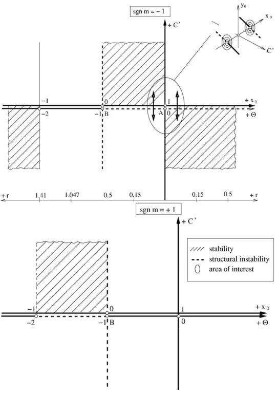
Assuminga11 <0,a12a21> 0the stability can be achieved e.g. forsgnm=−1andC′< 0. Detailed analysis will be done further for the simpler case µ → 0 — see Fig. 1. ForC′ =
0 ⇒ yeq = 0 ⇒ a11 = 0we have according to Grobman-Hartman theorem bifurcation (the equilibrium point is not hyperbolic — real part of the eigenvalue is zero). It can be shown that the conditions for the existence of the Hopf bifurcation usually cited (e.g. [8]) are fullfiled:
The first condition for the existence of Hopf’s bifurcation
• zero RHS of the equations (9) and (10) forxeq,yeqgiven by equations (11) and (12) and
C′= 0is obviously satisfied.
• pure imaginary eigenvalues forC′= 0exist if
−4a12a21>(a11)2 (18)
• condition of transversality for the real part of the eigenvalues has the form
∂a11 ∂C =
∂ ∂C
Cµ (1 + Θ)
2(rµ+ 1)(Θ2µ+ 1)
(rµ+ 1)[µ(Θ + 1)Θ−1] + 1
= 0 (19)
and it is fulfiled forµ= 0,−1 r,−
1
Θ2. The experimental results did not confirm the existence of
the non-degerated Hopf’s bifurcation and therefore the deeper analysis is necessary. We will do it for the following two cases:
• At first we will analyse the above mentioned system with the Fung’s formula (µ = 0) using multiple scale method when the control parameterC′in the neighbourhood of zero is depending onε2according to the recommendation in [8].
2.2. Multiple-scale analysis —µ= 0,C′=ε2C2
We assume the following form of the solution
x = x0+εx1+ε2x2+ε3x3 (20)
y = y0+εy1+ε2y2+ε3y3 (21)
where0< ε≪1is the scalar parameter. All variables in (20) and (21) are function ofT0, T1, T2
where
T0 =t, T1=εt, T2=ε2t. (22)
Before substituting from (20) and (21) into (9) and (10) we find the approximation for the exponential function
eµ2(x−1) 2
∼
=eµ2(x0−1)201 +µ(x0
−1)(εx1+ε2x2+ε3x3)1
. (23)
Further we introduce the following expression forC′
C′=ε2C2. (24)
x0andy0are the fix point coordinates given in (11) and (12). Fory0we can write
y0=ε2C2J (25)
where
J = −µ
(rµ+ 1)[µ(Θ + 1)Θ−1] + 1 (26)
Substituting now from (20) and (21) into (9) and (10) respecting the scaling of time (22) and neglecting the terms with exponent ofεgreater then 3, we obtain
∂x0 ∂T0 +ε
∂x0 ∂T1 +ε
2∂x0 ∂T2 +ε
∂x1 ∂T0 +ε
2∂x1 ∂T1 +ε
3∂x1 ∂T2 +ε
2∂x2 ∂T0 +ε
3∂x2 ∂T1+ε
3∂x3 ∂T0 =
=−ε2x0C2J µ
-eµ2(x0−1)
2
a1+ 1.−ε3x0C2Jeµ2(x0−1) 2
a2 −εx0 y1
µe µ
2(x0−1) 2
a1+y1 µ
−
−x0ε2
C2+y1eµ2(x0−1) 2
a2+y2 µe
µ
2(x0−1) 2
a1+ y2 µ
−
−x0ε3
y1eµ2(x0−1) 2
a3+y2eµ2(x0−1) 2
a2+ y3 µe
µ
2(x0−1) 2
a1+ y3 µ
− (27)
−ε3x1C2J µ
-eµ2(x0−1)2
a1+ 1.−ε2x1 y1
µe µ
2(x0−1)2
a1+y1 µ
−
−ε3x1
C2+y1eµ2(x0−1)2
a2+y2 µe
µ
2(x0−1)2
a1+y2 µ
−ε3x2 y1
µe µ
2(x0−1)2
a1+y1 µ
where
a1=µx2
0−µx0−1 (28)
a2= 2x0x1−x1+ (x0−1)x1(µx2
0−µx0−1) (29)
a3= 2x0x2+x2
1−x2+µ(x0−1)x1(2x0x1−x1) + (x0−1)x2(µx20−µx0−1) (30)
a4= 2x0x3−2x1x2−x3+µ(x0−1)x1(2x0x2+x2
1−x2) + (31)
+µ(x0−1)x2(2x0x1−x1) + (x0−1)x3(µx2
and similarly fory
∂y0 ∂T0 +ε
∂y0 ∂T1 +ε
2∂y0 ∂T2 +ε
∂y1 ∂T0 +ε
2∂y1 ∂T1 +ε
3∂y1 ∂T2 +ε
2∂y2 ∂T0 +ε
3∂y2 ∂T1+ε
3∂y3 ∂T0 =
=−
r−µ1eµ2(x0−1) 2
−1
+ (32)
+ε(x0−1)x1eµ2(x0−1)2+ε2(x0−1)x2e2µ(x0−1)2+ε3(x0−1)x3eµ2(x0−1)2
Now we compare the members with the same exponent ofε. We obtain three following systems of equations (remember thatx0andy0are constants!).
Forε1:
∂x1 ∂T0 +y1
x0 µ
-eµ2(x0−1)2
a1+ 1. = 0, (33)
∂y1
∂T0 = x1(x0−1)e µ
2(x0−1)2.
(34)
Forε2:
∂x2
∂T0 +y2b4 = − ∂x1
∂T1 −x0C2b1−y1x1b2+y1x 2
1b3, (35)
∂y2
∂T0 −x2(x0−1)e µ
2(x0−1) 2
= −∂T1∂y1. (36)
where
b1 = J µ
-eµ2(x0−1)
2
a1+ 1.+ 1, (37)
b2 = x0eµ2(x0−1) 20
2x0−1 +x0(µx20−µx0−1) 1
, (38)
b3 = x0eµ2(x0−1) 2
(µx20−µx0−1), (39)
b4 = x0 µ
-eµ2(x0−1) 2
a1 −1.. (40)
Forε3:
∂x3 ∂T0 +
∂x1 ∂T2+
∂x2
∂T1 = −x0C2Je µ
2(x0−1)2
a2 −
−x0
y1eµ2(x0−1) 2
a3+y2eµ2(x0−1) 2
a2+y3 µe
µ
2(x0−1) 2
a1+ y3 µ
−
−x1C2J µ
-eµ2(x0−1)
2
a1+ 1.− (41)
−x1
y1eµ2(x0−1) 2
a2+y2 µe
µ
2(x0−1) 2
a1+y2 µ − −x2 y1 µe µ
2(x0−1) 2
a1+y1 µ , ∂y3 ∂T0 + ∂y1 ∂T2+ ∂y2
∂T1 = (x0−1)x3e
µ
2(x0−1) 2
From (33) and (34) we obtain the second order equation forx1:
∂2x1 ∂T2 0
+ Ω2x
1= 0 (43)
where
Ω2 = (x0−1)x0 µe
µ
2(x0−1)2
-eµ2(x0−1)2
a1+ 1.. (44)
The solution is then
x1 = K1cos ΩT0−K2sin ΩT0 (45)
y1 = D(K1sin ΩT0+K2cos ΩT0) (46)
whereK1(T1, T2),K2(T1, T2)and
D= x0 Ω
µ 0
eµ2(x0−1) 2
a1+ 11. (47)
Now we will put this solution into (35) and (36). We can see, that the so called secular terms (terms containingsin ΩT0cos ΩT0)are only the derivatives on the right sides of these equa-tions (other terms contain products ofx1, y1and therefore goniometric functions with2ΩT0and higher). The secular terms have to be zero and the sufficient condition for this is
∂K1 ∂T1 =
∂K2
∂T1 = 0⇒K1(T2), K2(T2) (48)
The solution of the remaining system of equations x2, y2 are the periodical function with the frequency2ΩT0. Next step would be insertingx1, y1from (45) and (46) andx2, y2into (41) and (42):
∂x3 ∂T0 +
∂x1
∂T2 =−x0C2Je µ
2(x0−1)2
a2 −
−x0y3 µ
-eµ2(x0−1)2
a1+ 1.−x1C2J µ
-eµ2(x0−1)2
a1+ 1.−
(49)
– . . . terms with frequency2Ωor higher
∂y3 ∂T0 +
∂y1
∂T2 = (x0−1)x3e µ
2(x0−1) 2
.
The corresponding equation of the second order is
d2x 3
dT2
0 + Ω
2x3 = x0
µ
-eµ2(x0−1) 2
a1+ 1.∂y1
∂T2−x0C2Je
µ
2(x0−1) 2∂x
1
∂T0[2x0−1 + (x0−1)a1]−
−∂x1
∂T0
C2J
µ
-eµ2(x0−1)2a1+ 1
. − ∂2
x1
∂T2∂T0±. . .
(50) The secular terms on the RHS of (50) should be equal to zero. Inserting from (45) and (46) and comparing the coefficients bysin ΩT0,cos ΩT0we obtain the equations forKi
K′
iA+KiB= 0 (51)
whereK′
i=∂Ki/∂T2;i= 1,2and
A= Ω +Dx0
µ
-eµ2(x0−1)2
a1+ 1., B= ΩC2J*x0eµ2(x0−1)
2
[2x0−1 + (x0−1)a1] +1 µ
-eµ2(x0−1) 2
(51) is the special form of the so calledreconstituted amplitude equations[7] which is an asymptotic representation of a reduced dynamical system
˙
K1 ˙ K2
= ˙K=G(K(ε), C(ε)). (53)
The reconstituted amplitude equations allow generally to reduce the number of freedom to the codimension (that is the number of the pure imaginary and zero eigenvalues of (14), (15)). In this way this approach is equivalent to other reduction methods e.g. center manifold method. The condition (51) can be integrated and finally we obtain
Ki=Ki0e−BAT2
. (54)
1. If the exponent is negative thenKitend to zero and the equilibrium point is stable.
2. If the exponent is positive thenKigrowth and the equilibrium point is unstable.
3. If the exponent is zero (e.g. forC2= 0)than the solution can be approximated by
x = x0+x1=x0+K1cos ΩT0−K2sin ΩT0, (55)
y = y0+y1=y0+D(K1sin ΩT0+K2cos ΩT0). (56)
This corresponds with the numerical experiments as will be shown further.
2.3. Stability analysis forµ→0
Applying the limit procedureµ→0on (9) and (10) we obtain the equations
˙
x = −x-C′+ y
2
x2−1.
(57)
˙
y = sgnm
r−12(x−1)2
(58)
The equilibrium point has the coordinates
x0 = 1 + Θ, y0=− 2C
′
2Θ + Θ2 where Θ =±
√
2r. (59)
Equations in variations have the form (14) and (15) where
a11 = 2C′
(1 + Θ)2
Θ(2 + Θ), (60)
a12a21 = 1
2sgnmΘ
2(1 + Θ)(2 + Θ). (61)
Stability conditionsa11<0,a12a21<0— see (17) — are fullfiled if
Θ>0andsgnm <0andC′<0; −1<Θ<0andsgnm <0andC′>0; −∞<Θ<−1andsgnm <0andC′<0; −1<Θ<0andsgnm >0andC′>0;
(62)
The situation in the parameter space is shown on Fig. 1. Non-hyperbolicity condition — that is zero real part of at least one of the eigenvalues (17) — is fullfiled fora11= 0∧a12a21≤0or
a12a21= 0that is forC′= 0orΘ =−1∧Θ = 0orΘ =−1orΘ =−2. While the variables
x0, y0have to be positive, we will concentrate our attention on the neiboroghood of the pointA
2.4. Multiple-scale analysis forµ→0,C′=ε2C2
We apply the limit procedureµ→ 0on the above procedure and we obtain thereconstituted amplitude equationsin form
2ΩK′
i+ 1 2
3Θ2+ 6Θ + 2
Θ(Θ + 1)−rKi= 0 (63)
which is the limit of (51). The discussion leads to the same consequences as above.
2.5. Multiple-scale analysis forµ→0,C′=εC1
We try now to analyse the influence of the order ofC′and insertC′=εC1. The corresponding equations are
∂x0 ∂T0 +ε
∂x0 ∂T1 +ε
2∂x0 ∂T2 +ε
∂x1 ∂T0 +ε
2∂x1 ∂T1 +ε
3∂x1 ∂T2 +ε
2∂x2 ∂T0 +ε
3∂x2 ∂T1+ε
3∂x3 ∂T0 =
=−εx 0
C1J µ
-eµ2(x0−1)
2
a1+ 1.−ε2x0C1Jeµ2(x0−1) 2
a2 −
−εx0C1−εx0
y1 µe
µ
2(x0−1) 2
a1+ y1 µ
−
−x0ε3C1Jeµ2(x0−1) 2
a3 −x0ε2
y1eµ2(x0−1) 2
a2+ y2 µe
µ
2(x0−1) 2
a1+y2 µ
−
−x0ε3
y1eµ2(x0−1)2
a3+y2eµ2(x0−1)2
a2+ y3 µe
µ
2(x0−1)2
a1+ y3 µ
− (64)
−ε2x1C1J µ
-eµ2(x0−1)
2
a1+ 1.−
−ε2x1C1−ε2x1C1Jeµ2(x0−1)2
a2 −ε2x1 y1
µe µ
2(x0−1)2
a1+y1 µ
−
−ε3x1
y1eµ2(x0−1)2
a2+y2 µe
µ
2(x0−1)2
a1+ y2 µ
−ε3x2C1J µ
-eµ2(x0−1)2
a1+ 1.−
−ε3x2C1−ε3x2 y1
µe µ
2(x0−1)2
a1+ y1 µ
Using the similar approach as in the previous case we obtain the reconstituted amplitude equa-tion in form:
K′
i(1 +DΩ)−C1Ki[. . .] = 0; [. . .] = 2
x0(x0−1)
Θ(Θ + 2). (65)
Integrating equation (65) we obtain
Ki=Ki0exp
C1 [. . .]
1 +DΩT1
. (66)
We can see, that in this problem the result does not depend on the order ofC′.
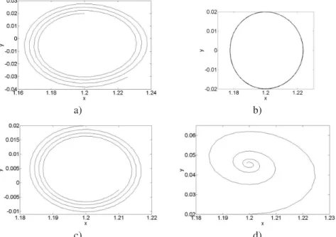
3. Numerical experiments
On the following figures we can observe the influence of C on the phase portrait in the neigh-bourhood of the bifurcation pointC= 0.
a) b)
c) d)
Fig. 2. Phase portrait forC={0.001,0,−0.001,−0.01}; starting pointx0= 1.2,y0= 0.02,µ= 0.1, r= 0.02
4. Conclusion
From the above demonstrated analysis we can extract conclusions:
1. In the presented cases the conditions (18), (19) do not justified the existence of the non-degenerated Hopf’s bifurcation. This was proved via multiple-scale method and con-firmed in numerical experiments. The reason is that also the fourth condition for the existence of this bifurcation has to be fulfilled: The bifurcation point should to be asymp-totically stable — see e.g. [9]. We have shown that this is not the case.
2. The order of the approximation of the control parameter in this case did not influence the qualitative description of the system behaviour in the neiborough of the equilibrium points.
3. Both studied cases — with Fung’s formula for the free energy potential and with the quadratic one — have the same qualitative properties.
4. The generalized external remodelling force influences essentially the phase portrait of the both dynamical systems. Especially interesting is the stable periodic motion for the zero value of this remodeling force.
5. On the other side it is necessary to stress that this phenomenon can be observed only if the change of stiffness is assumed!
Acknowledgements
This paper has been supported by the project MSM 4977751303. The authors would like to ex-press thanks to the anonymous reviewer for his very valuable comments and recommendations.
References
[1] A. DiCarlo, S. Quiligotti, Growth and balance. Mechanics Research Communications 29, Perga-monPress, 2002, pp. 449–456.
[2] M. Forcinito, M. Epstein, W. Herzog, Can a rheological muscle model predict force depres-sion/enhancement? Journal of Biomechanics 31 (1998) 1 093–1 099.
[3] J. Rosenberg, L. Hyncik, Contribution to the simulation of growth and remodelling applied to muscle fibre stimulation. In: Short communication of the 1st IMACS International Conference on Computational Biomechanice and Biology ICCBB 2007, Sept. 10–13, 2007, Plzeˇn, pp. 1–4. [4] F. Marˇs´ık, I. Dvoˇr´ak, Biothermodynamika. Academia, Praha, 1998.
[5] W. Herzog, Force enhancement following stretch af activated muscle: Critical review and proposal for mechanisms, Medical & Biological Engineering & Computing 2005, Vol. 43, 173–180. [6] J. Rosenberg, L. Hyncik, Modelling of the piezo-effect based on the growth theory. In:
Engi-neering Mechanics 2008, National Conference with international participation, May 12–15, 2008, Svratka, Czech republic.
[7] A. Luongo, A. Paolone, On the Reconstitution Problem in the Multiple Time-Scale Method, Non-linear Dynamics 19, 1999, pp. 133–156.
[8] A. Nayfeh, B. Balachandran, Applied nonlinear dynamics. John Wiley, 1995.