www.ann-geophys.net/24/3011/2006/ © European Geosciences Union 2006
Annales
Geophysicae
Cluster survey of the mid-altitude cusp: 1. size, location, and
dynamics
F. Pitout1, C. P. Escoubet2, B. Klecker1, and H. R`eme3
1Max-Planck-Institut f¨ur extraterrestrische Physik, Giessenbachstraße, 85741 Garching, Germany 2European Space Agency, Keplerlaan 1, 2201 AZ, Noordwijk, The Netherlands
3Centre d’´etude Spatiale des Rayonnements, 9, avenue du Colonel Roche, BP 4346, 31028 Toulouse Cedex 4, France
Received: 6 June 2006 – Revised: 24 August 2006 – Accepted: 6 September 2006 – Published: 22 November 2006
Abstract.We present a statistical study of four years of Clus-ter crossings of the mid-altitude cusp. In this first part of the study, we start by introducing the method we have used a) to define the cusp properties, b) to sort the interplanetary magnetic field (IMF) conditions or behaviors into classes, c) to determine the proper time delay between the solar wind monitors and Cluster. Out of the 920 passes that we have analyzed, only 261 fulfill our criteria and are considered as cusp crossings. We look at the size, location and dynamics of the mid-altitude cusp under various IMF orientations and solar wind conditions. For southward IMF,Bzrules the
lat-itudinal dynamics, whereasBy governs the zonal dynamics,
confirming previous works. We show that when|By|is larger
than|Bz|, the cusp widens and its location decorrelates from By. We interpret this feature in terms of component
recon-nection occurring underBy-dominated IMF. For northward
IMF, we demonstrate that the location of the cusp depends primarily upon the solar wind dynamic pressure and upon the Y-component of the IMF. Also, the multipoint capability of Cluster allows us to conclude that the cusp needs typically more than ∼20 min to fully adjust its location and size in response to changes in external conditions, and its speed is correlated to variations in the amplitude of IMF-Bz. Indeed,
the velocity in◦ILAT/min of the cusp appears to be propor-tional to the variation inBzin nT: Vcusp=0.0241Bz. Finally,
we observe differences in the behavior of the cusp in the two hemispheres. Those differences suggest that the cusp moves and widens more freely in the summer hemisphere.
Keywords. Magnetospheric physics (Magnetopause, cusp, arid boundary layers; Magnetospheric configuration and dy-namics; Solar wind-magnetosphere interactions)
Correspondence to:F. Pitout ([email protected])
1 Introduction
The cusp regions play a major role in solar wind-magnetosphere coupling. In fact, they are the regions through which the magnetosheath plasma has direct access to the magnetosphere and the ionosphere. Therefore, a good un-derstanding of these regions opens the doorway to the key is-sues of solar wind-magnetosphere-ionosphere coupling (e.g. review by Smith and Lockwood, 1996).
Cusp location and dynamics are a known topic and al-though this was not the primary goal of our study, we have decided to report about this in this first paper, with the in-tent not to redo what has already been done, but to present data in an original manner and to take advantage of the qual-ity of Cluster data and its multipoint capabilqual-ity. Incidentally, this is the first systematic statistical study of the mid-altitude cusp, thereby bridging previous work done at low and high altitudes.
1.1 Cusp size
The size of the cusp obviously depends on the altitude one considers. With its funnel-like shape, the cusp may be as broad as several Earth radii at high-altitude (Chen et al., 2005) and reduces to a few hundred kilometers in the iono-sphere (Newell and Meng, 1994).
Another crucial parameter, especially when it comes to the cusp longitudinal size, is the length of the reconnection line (X-line) at the magnetopause. Although the statistical results by Newell and Meng (1994) suggested that the cusp is on av-erage relatively narrow in terms of MLT, other authors have reported a very wide cusp footprint due to a much extended X-line (Crooker et al., 1991; Maynard, 1997).
and explained that the cusp is actually wider for northward than for southward IMF. The explanation comes from the enhanced convection under southward IMF which does not allow all the injected magnetosheath particles to reach the lower altitudes.
1.2 Cusp latitudinal location and dynamics
Although alternative explanations have been put forward in the past, suggesting that substorm activity was the main driver for cusp dynamics (Eather, 1985; Stasiewicz, 1991), large-scale latitudinal dynamics of the cusp in relation to the IMF orientation are no longer questioned and are now relatively well understood. Many studies involving vari-ous instruments and techniques have dealt with this topic for the past 30 years or so: low-altitude satellites (Escou-bet and Bosqued, 1989; Newell et al., 1989), mid-altitude satellites (Formisano and Bavassano-Cattaneo, 1978; Pitout et al., 2006), high-altitude satellites (Zhou et al., 2000; Palm-roth et al., 2001), space-borne imagers (Bobra et al., 2004) or ground-based optical instruments (Sandholt et al., 1983, 1994; McCrea et al., 2000, and references therein).
Whatever the hypothesis of magnetic reconnection one considers, the IMF orientation controls the location of the reconnection site at the Earth’s magnetopause and thus di-rectly determines the location of the cusp region. Obviously, as a consequence, cusp dynamics are extremely sensitive to changes in the IMF orientation. The component of the IMF which controls the cusp latitudinal location and dynamics is mainlyBz(Newell et al., 1989; Zhou et al., 2000; Palmroth
et al., 2001).
For southward IMF, the equatorward boundary of the cusp is very sensitive to the amplitude of the Z-component of the IMF. This is explained in terms of magnetic erosion at the dayside magnetopause: magnetic reconnection near the sub-solar magnetopause (between the two cusps) tends to erode the Earth’s magnetic field (Burch, 1973). This happens when the time scale for reconnection is shorter than the convec-tion time scale. Thus, the outermost closed field line ends up closer to the Earth. By mapping down to the magneto-sphere, this means an open-closed field line boundary (OCB) at lower latitude. Observations show that the more negative the IMFBzis, the lower in latitude the cusp finds itself.
For northward IMF, with the reconnection site at a much higher latitude, the whole cusp is also at a higher latitude but its location is then less sensitive to the magnitude of the Z-component and its footprint in the ionosphere is rather stable at around 77 MLAT (Newell et al., 1989).
Other parameters come into play in determining the cusp latitudinal location. The dipole tilt angle (Newell and Meng, 1989; Zhou et al., 1999) introduces a shift. For instance, when the dipole tilts sunwards, the cusp is shifted poleward in the Northern Hemisphere and equatorward in the Southern Hemisphere. The Y-component of the IMF also seems to have an influence: for largeBy, the cusp finds itself away
from noon (as we shall see in the next section) but also at a slightly lower latitude (Zhou et al., 2000; Wing et al., 2004), unlike predictions made by Rodger et al. (2000).
The solar wind pressure may also account for the cusp lat-itudinal location by moving the magnetopause standoff dis-tance. A compressed magnetosphere, for instance, would mean a magnetopause closer to the Earth and therefore the first open field lines at a lower latitude (Newell and Meng, 1994). For instance, cusp precipitation are commonly ob-served at latitudes which are usually considered as auroral latitudes (65–70 MLAT) when a coronal mass ejection hits the Earth’s magnetosphere. (e.g. Meng, 1982).
1.3 Cusp longitudinal location and dynamics
The east-west component of the IMF also plays a very im-portant role since it is the one that determines the cusp zonal location and dynamics. In the frame of anti-parallel re-connection (Crooker, 1979), the X-line splits into two parts (one in each hemisphere) when the IMF has a nonzero Y-component. The sign of By then determines the zonal
lo-cation of the reconnection sites and thus the lolo-cation of the cusps (Newell et al., 1989). For a negativeBy, the
recon-nection site is in the dawn sector and the newly-opened field lines are dragged duskward. On the contrary, forBypositive,
the cusp moves duskward and its plasma flows dawnward (Moen et al., 1999). This description applies to the Northern Hemisphere; everything has to be inverted in the Southern Hemisphere.
For component reconnection (Gonzales and Moser, 1974; Sonnerup, 1974), the description above also applies aside from the X-line, which does not disrupt but runs across the dayside magnetopause (e.g. Moore et al., 2002). Indeed, the cusp has sometimes a much wider zonal extent than expected (Maynard et al., 1997; Wild at al., 2003) but there has been no conclusive evidence so far that cusps having a large MLT extent necessarily result from component reconnection.
At last, it seems that the azimuthal solar wind flow may also contribute to the zonal dynamics of the cusp by “push-ing” it dawn- or duskward accordingly (Lundin et al., 2001; Zong et al., 2004).
2 Methodology
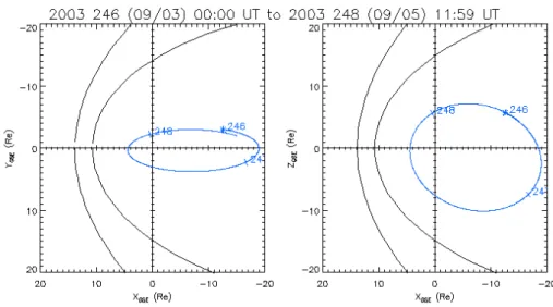
Fig. 1.Example of Cluster orbit (here in September 2003) leading to crossings of the cusp at middle altitude. Also shown are the magne-topause and the bow shock.
2.1 Cusp location and orbit selection
The orbits selected for this statistical study are taken from twelve months. For each of the years 2001 through 2004, we have studied 40 Cluster orbits from 1 July to 31 Octo-ber. This period of each year was chosen because the Cluster spacecraft were then orbiting at a middle altitude in the day-side magnetosphere (Fig. 1) between 16:00 and 08:00 MLT, respectively. As our initial motivation behind this survey was the identification of double cusps, we have deliberately taken a wide MLT interval (+/−4 h on both sides of magnetic noon), as reconnection sites leading to double cusps are ex-pected to be located far away from 12:00 MLT (under strong IMF-By). Out of the 160 orbits we have looked at, a
maxi-mum of 960 cusp crossings can be expected: 40 orbits/year times 4 years times 2 hemispheres times 3 spacecraft (no CIS sensors operational on SC2).
2.2 Cusp plasma properties
Determining the signature of the cusp at the middle altitude from particle data is not trivial. At a high altitude, one usu-ally uses the characteristic magnetic depletion as a signature. At a middle altitude, such an unambiguous signature does not exist. The criteria which we have used to define the cusp are based on previous studies on cusp plasma at mid-or low-altitudes (Fmid-ormisano and Bavassano-Cattaneo, 1978; Newell and Meng, 1988). We have used measurements per-formed by the CIS ion spectrometer (R`eme et al., 2001) and the Flux Gate Magnetometer (Balogh et al., 2001) on board the Cluster-2 spacecraft (Escoubet et al., 2001). The criteria are the following. We first need a condition on the particle density in the cusp. This condition is crucial and it will be in fact our primary criterion. Laasko et al. (2002) showed that density (electron density in their case) is a very reliable
parameter to identify the polar cusp. We know from statisti-cal studies at a high altitude (e.g. Lavraud et al., 2004) that the density in the exterior cusp is more or less equal to that in the magnetosheath. Since the magnetosheath plasma is a shocked and compressed solar wind plasma, we can expect densities in the cusp to be several times greater than the solar wind density. Results by Lavraud et al. (2004) suggest that the density in the cusp decreases with altitude down to solar wind values at∼8RE. Therefore, we impose the ion density
to be greater than or equal to that in the solar wind.
For many cases, a condition concerning the density was not sufficient to characterize the cusp; the density is some-times high in the low-latitude boundary layer (LLBL), too. We therefore impose additional conditions on both the mean energy and energy flux by nucleon of the downgoing ions:
– Pitch angles between 0 and 30◦ or between 150 and 180◦according to the hemisphere, northern and south-ern, respectively.
– Mean ion energy <Ei>∼2–3 keV and energy flux Fi
greater than 107ev/cm2s sr eV for energies ∼1 keV (Stenuit et al., 2001).
– At last, we do not expect many high energy ions in the cusp plasma (Lockwood and Smith, 1994), so ion en-ergy fluxes are imposed to be lower than 106ev/cm2 s sr eV for energies above 10 keV. This condition helps us in particular to differentiate the closed LLBL and the cusp for northward IMF, when the two layers are some-times difficult to separate.
2.3 Determining the prevailing IMF
Fig. 2. Magnetic local time (MLT) of each cusp crossing versus time. Crossings occurring in the Northern and Southern Hemi-spheres are shown in black and red, respectively.
Fig. 3.Location of all cusp crossings as a function of magnetic lo-cal time (MLT) and invariant latitude (ILAT). Black and red desig-nate crossings which occurred in the Northern and Southern Hemi-sphere, respectively.
wind plasma instrument (SWE) on board the ACE spacecraft. The propagation time from ACE to Cluster is first roughly estimated by dividing the solar wind bulk velocity by the distance between L1 and the dayside magnetosphere. When necessary, we check this lag by comparing ACE data to ei-ther Geotail data when suitably positioned in the near-Earth upstream solar wind or to ground instruments. Based on this, we sort any given cusp crossing among four classes of IMF behavior:
a) Steady southward IMF during the whole cusp crossing. b) Steady northward IMF during the whole cusp crossing. c) Rotating IMF. This behavior is chosen when one given
change in the IMF orientation is clearly identified as oc-curring during the cusp crossing and as being responsi-ble for a cusp discontinuity (presumably due to the mo-tion of the latter).
d) Highly variable IMF. Some of the cusp crossings we found occur under very variable IMF to such an extent that we cannot isolate the IMF turning(s) responsible for the change(s) in cusp morphology.
Fig. 4. Altitude and velocity of the satellites when they encounter the cusp in the Northern (black) and Southern (red) hemispheres.
3 Overview of cusp crossings
Using the method described in the previous section, 960 passes in the mid-altitude dayside magnetosphere were ex-amined. Out of those 960 passes, only 261 were identified as cusp crossings, representing ∼27% of the passes. Over the time period we have analyzed, they were distributed as follows: 2001: 49; 2002: 62; 2003: 84; 2004: 66.
The identified cusp crossings occur under the four classes of IMF conditions with the following distribution: steady southward: 111; steady northward: 46; rotating: 33; highly variable: 71.
Figure 2 shows the magnetic local time (MLT) at which all 261 crossings were observed. We see, as expected from orbit data obtained from the Joint Science Operation Center (JSOC), that Cluster flies through the dayside magnetosphere in the morning sector in July and progressively drifts towards noon in early September and the afternoon sector later on.
We have projected in Fig. 3 all cusp crossings on a MLT vs. invariant latitude (3) plot. Crossings occurring in the Northern and Southern Hemispheres are colored in black and red, respectively. At a first glance, we see that most of the recorded cusps are located between 10:00 and 14:00 MLT and 75◦and 80◦ILAT.
An important aspect one needs to bear in mind for the forthcoming analysis is that the apogee of the Cluster orbit is slightly below the equatorial plane. Consequently, the cusp is crossed neither at the same altitude, nor at the same speed in the two hemispheres. This is clearly visible in Fig. 4, which shows the altitude of each crossing versus the speed of the spacecraft. All crossings occurring in the Southern Hemi-sphere (in red) occur between 5.5 and 8RE, whereas those
Fig. 5.Panel showing for each crossing, from top to bottom, the al-titude and velocity of the spacecraft, the duration of the cusp cross-ing in minutes, the cusp latitudinal width in degrees (difference be-tween the locations of the poleward and the equatorward bound-aries), and the latitudinal width in thousands of kilometers (duration of the crossings times the velocity of the spacecraft).
Our data set consists of 146 crossings in the Northern Hemi-sphere and 115 in the Southern HemiHemi-sphere.
4 Crossing duration and cusp size
Cluster measures the latitudinal extent of the cusp at a sin-gle longitude. What we can infer from the duration of the crossing is therefore the latitudinal width of some part of the cusp. Figure 5 displays for each crossing, from top to bot-tom, the altitude of the spacecraft and its velocity, the du-ration of the cusp crossing in minutes, the latitudinal width in degree, and the latitudinal width (obtained by multiplying the speed of the spacecraft by the duration of the crossings) in thousands of kilometers. Even if, on average, a cusp cross-ing lasts 14 min and the cusp width is 1.96◦or 3.43×10³km (0.54RE), Fig. 5 exhibits a great variability, which we are
going to analyze and comment on now.
Fig. 6. Cusp latitudinal width as a function of IMF-Bz. Red dots
show average widths binned by IMFBz.
We have calculated the mean cusp width for both north-ward and southnorth-ward IMF cases. We find 2.10◦ and 1.58◦, respectively. This is in agreement with results by Newell and Meng (1987). We can even determine a relation between the cusp width and the Z-component of the IMF, although the correlation is not very high. Figure 6 shows the cusp width in degrees versus IMF-Bz. The red dots represent averaged
cusp width by +/−5 nT bins. Those red dots may be interpo-lated nicely by a straight line whose equation is:
Cusp width=0.052Bz+1.87. (1)
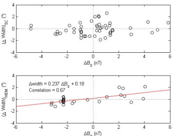
In order to have an insight into the rapidity of the reaction of the cusp width to changes in the IMF, we have plotted in Fig. 7 the variations of the cusp width versus the corre-sponding variations in IMF-Bz. The top panel shows
vari-ations (1width)SC between all possible pairs of spacecraft
crossing the same cusp (3 pairs of differences at most for each pass), whereas the bottom panel shows variations (1 width)HEM between all possible pairs of spacecraft (it may
be the same spacecraft) crossing the southern cusp first and then the northern cusp on the same orbit (9 pairs of differ-ence at most for each orbit). Obviously, only cases where the IMF was measured (i.e. steady or rotating IMF conditions) were considered, which considerably limits the number of data points. The cusp is expected to widen with increasing Bz and becomes narrower with decreasingBz, so we ought
Table 1.: Cusp width in thousands of km for both hemispheres as a function of the IMF behavior.
All IMF SteadyBz<0 SteadyBz<0 Rotating Rotating N->S Rotating S->N Variable
Northern Hemisphere 2.85(146) 2.27(77) 3.39(21) 3.65(21) 5.09(6) 2.63(11) 3.09(27) Southern Hemisphere 4.18(115) 3.30(34) 3.57(25) 3.47(12) 4.06(7) 2.60(4) 5.36(44)
Fig. 7. Variations of the cusp width versus variations in IMF-Bz.
The top panel shows variations between pairs of spacecraft crossing the same cusp, whereas the bottom panel shows variations between the southern and the northern cusps on the same orbit, as well as the linear fit of the data points (in red). Only cases occurring under steady or rotating IMF are considered.
conditions. The linear fit of the data points gives the follow-ing relation (with a good correlation coefficient of 0.68):
1width=0.2371Bz+0.18. (2)
Newell and Meng (1987) observed this with successive passes of DMSP satellites, i.e. 101 min apart. All this sug-gests that the time scale for the cusp to fully reconfig-ure is somewhere between a couple of tens of minutes and ∼100 min.
In order to look at possible hemispheric/altitude and IMF effects, we have averaged the latitudinal width of the cusp for several conditions. Results are shown in Table 1, which show the cusp latitudinal width in thousands of kilometers for var-ious IMF behaviors and for both hemispheres. The number of occurrences of each case is shown between parentheses. Note that we prefer, for accuracy’s sake, to handle here the width in distance (calculated from the speed of the spacecraft and the duration of the crossings).
First of all, we see what was foreseen: the cusp is wider when it is crossed in the Southern Hemisphere because the spacecraft are then at a higher altitude (∼8RE instead of
∼5REin the Northern Hemisphere). This is observed when
Table 2.: Mean cusp width (in thousand of km) for two steady IMF orientations and for the two hemispheres before and after autumnal equinox.
Pre-equinox Post-equinox north south north south SteadyBz<0 2.23(60) 3.13(29) 2.41(17) 4.21(5)
SteadyBz<0 3.80(19) 3.89(14) 3.08(2) 3.29(11)
all IMF are considered, for both steady southward and north-ward IMF, and for variable IMF. For rotating IMF, the results show a wider cusp in the Northern Hemisphere. Besides, the motion of the cusp relative to the spacecraft motion does not seem to play any role. We recall that Cluster flies through the dayside magnetosphere from south to north, so one could expect, for a rotation from a southward to a northward IMF, for instance, to find a wider apparent cusp in the Northern than in the Southern Hemisphere (as the cusp would move northward, i.e. in the same direction of the spacecraft in the Northern Hemisphere, unlike in the Southern Hemisphere where the cusp and the spacecraft would move in opposite directions). The most relevant seems then to be the condi-tions before the change: wide cusp for rotation from north to south, narrow for rotations from south to north. This shows again that the cusp needs some time to adjust itself to new IMF conditions. Note that there may be some hysteresis ef-fect of the magnetosphere involved as well, as suggested by Palmroth et al. (2006).
Also, we would like to discuss the possible role of the sea-son, because if the cusp is expected in our case to be wider in the Southern Hemisphere, the speed of the magnetosheath flow, which determines the length of time an open field-line spends in the cusp, should also intervene in determining partly the width of the cusp (Newell and Meng, 1987). Now magnetosheath flow is supposed to be faster near the cusp of the winter hemisphere than that of the summer hemisphere (Taylor and Cargill, 2002) and therefore, the cusp ought to be narrower in the winter hemisphere. In other words, does the seasonal effect counterbalance the altitude difference as far as the cusp width is concerned? Table 2 helps us investi-gate the possible “conflict” between the two aspects. It shows the mean cusp width for each hemisphere, for IMFBz
hemisphere is colored grey. Before equinox and forBz<0,
the cusp is wider in the Southern Hemisphere (3.13×10³km against 2.23 in the north) as expected; yet, this is where the magnetosheath flow is the fastest. The altitude effect domi-nates. After equinox, still forBz<0, the difference in width
between the two cusps is significantly larger (4.21×10³km in the south, which is now the summer hemisphere, against 2.41 in the north). Here, the seasonal effect has clearly inter-vened to make the southern cusp even wider. ForBz>0, the
means of the cusp widths are very similar in the two hemi-spheres before the equinox. Again, the seasonal effect affects the cusp width in the Southern Hemisphere: field lines which are newly reconnected in the southern lobe are swept away faster by the strong magnetosheath flow. This is also true for the Northern Hemisphere but the magnetosheath flow is then expected to be slower. After the equinox, the values once again confirm our explanation, although the statistics are very poor (only two cases for the Northern Hemisphere).
5 Cusp location and dynamics
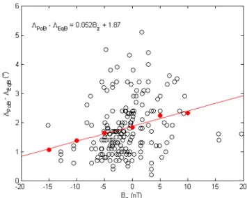
As already mentioned in the Introduction, the location of the cusp with respect to the IMF orientation is nothing new. However, in addition to the reasons already evoked, we think that it is worth performing the same kind of analysis as Newell et al. (1989), Zhou et al. (2000), or Palmroth et al. (2001). Those studies were made at different altitudes, so it will be interesting to compare our results with theirs and thereby, to compare the cusp dynamics at various altitudes. 5.1 Dipole tilt effect and corrected invariant latitude Before going into the statistics and their analysis, the effect of the dipole tilt angle has to be removed in order to isolate the IMF effects. To do so, one needs to determine the quan-titative contribution of a given inclination of the dipole to the observed invariant latitude of the cusp. This may be tricky, as the IMF effect may, in turn, come into play. To limit the contribution of the IMF, we may, as in previous studies, plot the location of the cusp as a function of the dipole tilt only for northward IMF cases, for which the cusp latitudinal lo-cation is more or less stable. This does help but then the solar wind pressure should be of the same order of magni-tude for all selected cases because we know that the state of compression of the magnetosphere also affects the cusp lo-cation. Likewise, the MLT sector should be about the same for all samples, as an effect on the latitudinal location has been reported. Besides, all the authors already mentioned (Newell and Meng, 1989; Zhou et al., 2000; Palmroth et al., 2001) performed their studies on the location of the center of the cusp. Yet, the boundary between the cusp and the thick, dense LLBL is somewhat fuzzy under northward IMF. For this reason, we prefer to handle the location of the poleward boundary of the cusp, which, for northward IMF, appears
Fig. 8. Invariant latitude of the poleward cusp boundary versus dipole tilt angle for crossings corresponding to steady IMF whose clock angle is between−45 and 45◦(in GSM) and to a solar wind dynamic pressure smaller than 5 nPa. Black/red dots are from cross-ings in the Northern/Southern Hemisphere.
to be a sharp and clear boundary (Lavraud et al., 2002) and therefore, a more accurate parameter. All in all, in order to take into account all of these considerations, we have han-dled the invariant latitude of the poleward boundary (3PoB)
of the cusp only for crossings occurring for clock angles of the (steady) IMF between−45◦ and 45◦(in GSM) and for solar wind dynamic pressures smaller than 5 nPa.
Figure 8 shows the invariant latitude of the poleward boundary of the selected cusps (3PoB)versus the tilt angle
(8). The slope of the linear fit is 0.0907, thus, an increase of∼11◦in tilt angle8results in an increase/decrease of 1◦ in invariant latitude in the Northern/Southern Hemispheres. This correction is applied to the invariant latitudes of the equatorward and poleward boundary of the cusps observed. This is somewhat lower than the values found by Newell and Meng (1989) and Zhou et al. (1999) but larger than that found by Nˇemeˇcek et al. (2000). We remove this effect for each cusp crossing and handle corrected invariant latitudes3, as
3=ILAT+/−0.09078 (3)
(+ and−for the Northern and Southern Hemispheres, re-spectively).
We have to point out that we have used cusp crossings from both hemispheres in Fig. 8. We have just multiplied the tilt angles by−1 for the Southern Hemisphere. Besides, for a reason that we shall discuss later on, we notice that the data points corresponding to the Northern Hemisphere (black) are much more scattered than those for the Southern Hemisphere (red).
Fig. 9. Location of the equatorward (top) and poleward (bottom) cusp boundary as a function of the Z-component of the IMF. Only cases occurring under stable IMF conditions and for a solar wind dynamic pressure smaller than 5 nPa are plotted.
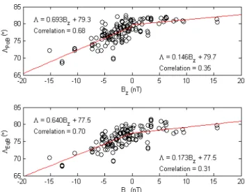
5.2 IMF-Bzdependence
A negative Z-component of the IMF is expected to enhance the reconnection process at the Earth’s magnetopause and therefore, to erode the magnetosphere magnetically, so that the reconnection region becomes closer and closer to the Earth. By projecting down to the ionosphere, this means that the footprint of the X-line becomes lower and lower in lati-tude. This is the basic concept. In practice, other parameters come into play in the location of the cusp and interfere, so to say, with theBzeffect, to such an extent that it may actually
be difficult to obtain an accurate qualitative view of the pure Bzeffect.
Figure 9 shows a scatter plot of the invariant latitude of both the equatorward and poleward edges of the cusp ver-sus IMF-Bz. Note that only cusp crossings occurring under
steady IMF and for a solar wind pressure smaller than 5 nPa have been plotted. For negative values ofBz, the cusp
loca-tion exhibits the expected dynamics: the localoca-tion of the cusp edges decrease in latitude withBzas follows:
3EqB=0.640Bz+77.5 (4)
3PoB=0.693Bz+79.3. (5)
For northward IMF (positiveBz), the behavior of the cusp is
more stable, its location is much less sensitive to variations in IMFBz. Although the linear fit indicates that the location of
the cusp should progress northward asBzincreases (positive
slope in right-hand side of both panels of Fig. 9), a look at the data points suggests the contrary, that is to say that the cusp remains rather stable or even moves slightly equatorward as Bzincreases! We should remark at this stage that there have
been some inconsistencies between previous studies on the
Fig. 10.Equatorward boundary of the cusp versus IMF-Bzfor the
Northern (top) and Southern (bottom) Hemispheres. Filled circles correspond toBydominated IMF. Only cases occurring under stable
IMF conditions are plotted.
Fig. 11.Variations of the location of the cusp equatorward boundary versus variations in IMF-Bz. As in Fig. 7, the top panel shows
vari-ations between pairs of spacecraft crossing the same cusp, whereas the bottom panel shows variations between the southern and the northern cusps on the same orbit. Only cases occurring under steady or rotating IMF are considered.
behavior of the cusp under northward IMF. This will be dis-cussed later on.
In order to investigate possible hemispheric differences, we have plotted in Fig. 10 the invariant latitude of the cusp equatorward boundary versusBz for each hemisphere
Fig. 12.Variations of the velocity of the poleward (top) and equator-ward (bottom) boundaries of the cusp as a function of the variation inBz. Only pairs of spacecraft crossing the same cusp not more
than 30 min apart and under steady or rotating IMF are considered.
other hand, the left-hand part of each panel (negativeBz)
presents interesting features. First of all, the linear fits have similar slopes, showing that the cusp behaves the same way in both hemispheres. On the other hand, there seems to be an asymmetry in the position of the cusp: it seems to be at a slightly higher latitude in the Southern Hemisphere: for Bz=0, the equatorward boundary is at 77.4◦in the north and
78.1◦in the south. However, this would need to be confirmed with more data points. At last and maybe more interestingly, as already noticed previously, the correlation is better in the Southern (0.82) than in the Northern (0.68) hemisphere.
We have taken advantage of the multipoint capability of the Cluster to investigate the reactivity of the cusp in re-sponse to changes inBz. We know that large-amplitude and
rapid changes in the IMF are accompanied by a fast response of the cusp (Pitout et al., 2006). We have compared the loca-tion of the cusp equatorward boundary of successive passes of the Cluster spacecraft through the same cusp, on the one hand, and we have compared the location of the cusp between the Southern and Northern Hemispheres during the same or-bit, on the other hand (same technique as for Fig. 7 and there-fore, the same pairs of spacecraft), as seen in Fig. 11. Succes-sive passes of the Cluster satellites through a given cusp (top panel) show the tendency: a decrease/increase inBz makes
the cusp move equatorward/poleward, although it is not the case for all the points. This may depend on the time differ-ences between the pair of passes taken. The tendency is much clearer when the two cusps are compared (bottom panel of Fig. 11). The cusp has then all the time in the world (∼4 h in fact) to adapt itself to the new IMF conditions. By fitting the data points in the latter case (bottom panel of Fig. 11), we find again a similar slope, 0.679, as in Eq. (4).
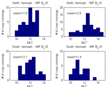
Fig. 13. Occurrence of cusp crossings sorted by Magnetic Local Times. Cusp crossings occurring under steady IMF are plotted.
Cases for which the duration between two successive passes is not too long are of particular interest in order to find the latitudinal velocity of the cusp while it responds to a given IMF change in the Z direction. Figure 12 displays the velocity of the cusp (calculated with pairs of spacecraft crossing the same cusp not longer than 30 min apart) suc-cessive passes not exceeding 30 min apart) as a function of the variation inBz. It suggests that the velocity of the cusp is
proportional to1Bz. Both the poleward and the equatorward
boundaries move at the same velocity (in◦/min/nT):
V =0.0241Bz. (6)
5.3 IMF-Bydependence
The zonal location of the cusp, in MLT, is shown in Fig. 13 for the two hemispheres (north on top, south at bottom), and for negative and positive IMFBy(left and right,
respec-tively). For each case, the mean MLT is given. Here again, only the cusp crossings occurring under steady IMF have been plotted. We find the well-known trend, i.e. the cusp is statistically found in the morning sector of the Northern Hemisphere for negativeBy (11.8 MLT on average) and in
the afternoon sector for positiveBy (12.5 MLT on average).
The opposite trend is observed in the Southern Hemisphere: 12.1 forBy<0 and 11.4 forBy>0). All this is a priori in
agreement with anti-parallel reconnection sites but we shall discuss later on the few cases that do not follow this trend.
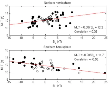
Another way to look at thisBy-effect is shown in Fig. 14,
which displays the MLT of each cusp crossing as a function of the Y-component of the IMF for the Northern and South-ern Hemisphere (top and bottom, respectively). Filled data points correspond to cases whereByis larger thanBzin
Fig. 14.Magnetic local time of cusp crossings (under steady IMF) as a function of IMF-By. Filled circles correspond to cases with |By|>|Bz|.
The linear fit is superimposed in red and the equation of the straight line is very similar for both hemispheres, with a co-efficient of “zonal mobility” of 0.087 (0.085) MLT/nT. For By=0, the cusp finds itself near noon in both cases.
It should be noted that the correlation coefficient is better in the Southern Hemisphere (−0.58) than in the north (0.35). Besides, cases where|By|>|Bz| are much more scattered,
particularly in the Northern Hemisphere, suggesting that the cusp becomes wider whenByis larger thanBz.
5.4 Solar wind dynamic pressure dependence
By considering all cusp crossings together, no obvious corre-lation is found between the location of the cusp and the solar wind dynamic pressure, because we face the same problem as in Sect. 5.1 when we removed the dipole tilt effect: the dynamics due to the magnetic erosion (Bz effect) may and
do interfere with the pressure effect. Yet, we do know that a high solar wind dynamic pressure (during storms, for in-stance) makes the cusp move to lower latitudes (e.g. Meng, 1982). In order to see a clear effect of the solar wind pres-sure on the cusp location, we consider only cusp crossings occurring under predominantly northward IMFs (clock an-gles between−45 and 45◦). Figure 15 shows the location of the cusp poleward (top) and equatorward (bottom) bound-aries as a function of the solar wind dynamic pressure. A dependency between the solar wind pressure chosen and the location of the cusp is clearly visible and the correlation fac-tors are excellent. The linear relations between the solar wind pressure (Psw)and the invariant latitude of the poleward and
equatorward boundaries of the cusp (3PoBand3EqB)are:
3PoB= −0.390Psw+82.1 (7)
Fig. 15. Location of the cusp poleward (top) and equatorward (bottom) boundaries for steady and positive Bz dominated IMF
(|θIMF|<45◦) as a function of the solar wind dynamic pressure.
3EqB= −0.503Psw+80.7. (8)
These relations confirm that the cusp moves down in lati-tude with increasing solar wind pressure and also show that it widens (the equatorward edge depends on the pressure with a greater coefficient (in absolute value) than the poleward edge).
We can note in Fig. 15 that the correlation coefficient is better for the poleward boundary (−0.90) than for the equa-torward boundary (−0.76), which confirms that the poleward boundary is a better parameter to describe the cusp dynamics under northward IMF (as mentioned in Sect. 5.1). These are also the best correlation coefficients obtained in this study.
6 Discussion
6.1 Number of cusp crossings
away from noon. Our MLT range being wider than the statis-tical cusp width (Newell and Meng, 1994), we could indeed easily miss it.
At last, an unfavorable IMF-By may move the cusp
to-wards the opposite MLT sector. This may occur, for in-stance, if Cluster is in the morning sector of the Northern Hemisphere and that a positive IMF-By “pushes” the cusp
towards the afternoon sector. Cluster will, in this case, miss the cusp. This also illustrates the relative narrowness of the cusp at those altitudes.
6.2 Dipole tilt angle effect on the cusp location
In Sect. 5.1, we found that a shift of 11◦ in the dipole tilt angle yields a shift of 1◦in the invariant latitude of the cusp
poleward boundary. This has to be compared to other stud-ies. Values as high as 14◦ tilt for 1◦ ILAT and 17◦ tilt for
1◦ILAT were found, respectively, by Zhou et al. (1999) and
Palmroth et al. (2001) whereas Nˇemeˇcek et al. (2000) found a lower value of 8◦tilt for 1◦ILAT. There are several elements that may account for these differences. First of all, these differences may arise from the fact that we have performed our study on the poleward boundary of northward IMF-cusps only. As emphasized by Palmorth et al. (2001), the location of the cusp equatorward boundary is not clear under north-ward IMF and even worse, it is instrument-dependent. Be-sides, it is well known that the solar wind density has a di-rect consequence on the size of the magnetosphere and thus, on the location of the footprint of the first open field lines, regardless of the IMF orientation. There have also been re-ports, although sometimes contradictory, on the role of the Y-component of the IMF, pushing the cusp in the morning or afternoon sector but also at higher (or lower, depending on the author) latitudes. To be as rigorous as possible and to re-move those undesirable effects, we have constrained our se-lection in terms of IMF clock angle and solar wind dynamic pressure (Sect. 5.1). This again may introduce differences. Apart from the study by Palmroth et al. (2001), in which a separation has been made between cases whereBy is large
or small, all the other studies did not contain such a discrim-ination, which we think is necessary.
At last, we have seen that the cusp does not behave the same way in the two hemispheres. The qualitative role of the dipole tilt may, under these conditions, depend on the fact that one or both hemispheres are taken into account for the analysis.
6.3 Cusp latitudinal location for southward IMF
The location of the equatorward edge of the cusp is a priori ruled by the location of the dayside magnetopause, which is determined by both the solar wind dynamic pressure and the Z-component of the IMF (through magnetic erosion). As we mentioned already, it is often difficult to separate the effects of each of them but one way to account for both would be
Fig. 16.Poleward and equatorward cusp boundaries versus magne-topause stand-off distance (from Shue et al. model). Filled circles correspond to cases with|Bz|>|By|. Only cases occurring under
stable IMF conditions are plotted.
to compare the location of the cusp with the magnetopause stand-off distance, for instance.
Figure 16 shows the latitude of the cusp poleward and equatorward boundaries (3PoBand (3EqB)versus the
stand-off distance given by the Shue et al. (1997) model for steady southward IMF. Circles are filled when the IMF clock angle is greater than 135◦in absolute value (|B
z|>|By|). The linear
fit of the circled data points is in red, the equation of which is given, together with the correlation coefficients. We can see that the location of the cusp correlates very well (∼0.7 for both boundaries) with the stand-off distance, but not bet-ter than withBzalone (Fig. 9), which is surprising knowing
that the location of the subsolar point takes the solar wind pressure into account, thus a priori a better description of the location of the first open field line.
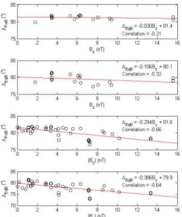
Lastly, we should point out that the correlation factors drop to 0.48 and 0.41, respectively, for the poleward and equator-ward boundaries when all data points are taken into account (Fig. 16). The distribution of the empty circles, at higher lati-tudes globally, emphasizes the role ofBywhen it dominates:
it moves the cusp to higher latitudes (see Sect. 6.5). 6.4 Cusp latitudinal location for northward IMF
Fig. 17. Invariant latitude of the cusp poleward and equatorward boundary as a function ofBz (two first panels) and|By|(two last
panels), all for steady and northward IMF.
of Bz increases (Zhou et al., 2000; Palmroth et al., 2001),
whereas others show the opposite (Newell et al., 1989). Like-wise, the poleward boundary is said to progress poleward as Bzincreases (Palmroth et al., 2001) or equatorward (Zhou et
al., 2000).
In the face of these disagreements, let us first look in detail at what could possibly affect the cusp location under north-ward IMF (apart from the solar wind dynamic pressure). If magnetic erosion in the lobe were effective, it would make the first open field line move at a higher latitude as the mag-nitude ofBzincreases. This is, by the way, the behavior we
obtain, like Newell et al. (1989), when we consider allBz>0
cases. This behavior ought to be emphasized by selecting cases for whichBzdominates (clock angle<45◦in absolute
value). In order to isolate this possible effect, we have plot-ted in the two first panels of Fig. 17 the location of the equa-torward and poleward boundaries of the cusp corresponding to stable andBz-dominating (|Bz|>|By|)IMFs, and to
so-lar wind pressures smaller than 5 nPa. We can see that not only the slope is negative (which rules out the possible role of magnetic erosion) but the correlation is poor, suggesting that in fact,Bzdoes not play any role in the cusp dynamics
for northward IMF.
Palmroth et al. (2001) have invoked an IMFBy-effect. We
have materialized this in the two bottom panels of Fig. 17.
They show the location of the equatorward and poleward boundaries of the cusp under northward IMF as a function the absolute value of IMF-By. As previously, only cases
cor-responding to stable IMF and with a moderate solar wind pressure (Psw<5 nPa) have been plotted. UnlikeBz,By
ap-pears to influence greatly the latitudinal location of the cusp: the cusp moves at lower latitudes with increasingBy. Note
that the correlation coefficient is much better than withBz.
The positive slopes which we obtained in Fig. 9 are there-fore more constrained by the cases nearBz=0 (some of which
are dominated byBy)than by some actual dependence onBz.
6.5 The role of IMF-Byon the latitude of the cusp
Several studies have underlined the role ofByin moving the
cusp equatorward as it increases (Zhou et al., 2000; Wing et al., 2004). On the contrary, Rodger et al. (2000) pre-dicted that the location of the cusp should migrate at higher latitudes asBy increases. In fact, these two former studies
mixed northward and southward IMF cases and we think this detail has its importance. We show in the previous section thatBydoes play a role under northward IMF in moving the
cusp at lower latitudes. We have plotted in the first panel of Fig. 18 the invariant latitude of the cusp equatorward bound-ary (3EqB)versus|By|for all cases corresponding to a steady
IMF (northward or southward) and to a solar wind pressure smaller than 5 nPa (like previously). We have averaged3EqB
for bins of|By|+/−2 nT separately for both northward (red
plain dots) and southward (blue) IMF and linearly fitted these mean values. We see that3EqBdecreases with|By|for both
cases. But this should be handled with caution: we know from the previous section thatBzplays no major role in the
cusp dynamics under northward IMF but this is far from the case for southward IMF. In order to reduce the effect ofBz,
we have plotted in the bottom panel of Fig. 183EqBversus
the sine of the absolute value of the IMF clock angle, which is zero when the IMF is purely “vertical” (along the z-axis in the (y,z) plane), and 1 when the IMF is purely “horizontal” (along the y-axis). The averaging method (sin|θIMF|+/−0.1)
and color codes are similar to those used for the top panel. We clearly see the effect of the orientation of the IMF. When it is along Z, the location of the cusp greatly depends on the sign ofBz, which is not surprising at all. But as sin|θIMF|
increases (i.e. asBy becomes larger and larger with respect
toBz), the locations of the cusp for northward and
south-ward IMF converge tosouth-ward a unique location, which is the location for an IMF totally horizontal (in the (y,z) plane). So when the IMF rotates from due north/south to due east or west, the cusp moves down/up in latitude, respectively. 6.6 Cusp latitudinal velocity in response to changes in
IMF-Bz
to the variation inBz(Fig. 12). Note that even if a change in Bz does not necessarily imply a change in the sign of Bz,
the velocity inferred must in fact come from cases whereBz
change sign or whereBzremain negative, because we know
that the motion of the cusp is very limited during northward IMF.
Recently, Escoubet et al. (2006) have reported the mo-tion of ion steps in response to a southward turning of the IMF as measured by Cluster at middle altitude. The first ve-locity measured, right after the turning was of the order of 0.43◦/min and then, the two following ones were of the or-der of 0.16◦/min (for a change inBzof about 5 nT). For the
same change, our relation (6) gives 0.12◦/min, which is fairly similar to the two last measurements.
We have to say that the method used to infer the velocities plotted in Fig. 12 may explain why we find lower values. In fact, in order to have enough data points, we have allowed a length of time of 30 min between two successive satellite passes; 30 min is probably a little longer than the time the cusp actually needs to fully reorganize. Velocities inferred from relation (6) may then be underestimated.
6.7 Cusp zonal dynamics and implication for merging We have shown that the cusp zonal dynamics agrees well with the previous results by Newell and Meng (1994) or Palmroth et al. (2001), for instance. Statistically speaking, we do observe that the cusp moves with the Y-component of the IMF and results from cited studies also consider a sta-tistical approach. However, on a case by case basis, we also see a non-negligible amount of cases which do not follow the expected trend. Where do they come from? First of all, the cusp may have a zonal width of a couple of hours in MLT, therefore, we don’t know, for a given cusp crossing, which part Cluster goes through. There may be another reason: as a matter of fact, we invoked, on the one hand, the large zonal extent of the cusp to explain why we observe it in the “wrong” sectors with respect to the IMFBy, and indeed, the
cusp may be very wide in local time (Maynard et al., 1997). On the other hand, we put forward its narrowness in Sect. 6.1 to explain why only one quarter of the potantial cusp cross-ings are actually identified as cusp crosscross-ings. There is here a contradiction that must reveal something else. While some works suggest that component and anti-parallel reconnection may occur simultaneously (Lockwood et al., 2003), recent results from Trattner et al. (2005) indicate that anti-parallel reconnection is the reconnection mode occurring by default, so to speak, or at least the one which dominates. When anti-parallel reconnection cannot operate efficiently, because of an unfavorable configuration (largeBy), then component
re-connection becomes dominant. We propose that those cases which do not follow the usual trend are not necessarily cases that should be ignored in the name of statistics, and could well have an important physical significance. We know that the reconnection line (X-line) may be greatly distorted and
Fig. 18.Invariant latitude of the cusp equatorward boundary versus
|By|(top) and sin|θIMF|(bottom). In red and blue are the binned
mean invariant latitudes and the corresponding linear fit for north-ward and southnorth-ward IMF, respectively. Only crossings under steady IMF are considered.
covers a large part of the magnetopause in the case of com-ponent reconnection. Cases off the statistical trend may re-sult from component reconnection (Bobra et al., 2004). This is precisely what we found in Sect. 5.3 and Fig. 14: cusps corresponding to cases whereByis greater thanBzare
basi-cally found everywhere, irrespective of the IMF orientation. This shows that the MLT sector somewhat decorrelates from By when the latter becomes large. This is much in favor of
an extended X-line, i.e. of component reconnection.
A last possibility involving only the strength of Bz
ex-ists, although we cannot verify it due to an insufficient num-ber of data points: Crooker et al. (1991) have shown that for strong southward IMF, the cusp local time extent can be much larger. For larger |Bz|, one expects more
subso-lar merging, compared to the smaller|Bz| situation, where
anti-parallel or higher latitude merging is more likely. The direct implication is the same: under subsolar reconnection, the cusp would be observed at a larger range of MLT. 6.8 Altitude and seasonal effects
We have noticed in Sect. 5 an interesting feature: in Fig. 10, the correlation between the IMF-Bz and the latitude of the
cusp equatorward boundary is greater in the Southern Hemi-sphere (0.82) than in the Northern HemiHemi-sphere (0.68). Like-wise, in Fig. 14, the correlation between the IMF-Byand the
MLT sector at which the cusp is observed is rather good in the Southern Hemisphere (−0.58), whereas it is poor in the Northern Hemisphere (0.35). We have already mentioned that cusp crossings in the Northern Hemisphere take place at lower altitudes (∼5RE)than in the Southern Hemisphere
also depends on the altitude: The magnetic field strength at high-altitude is much lower (3 order of magnitude) than at low altitude, therefore, field lines at high altitude are much more mobile and more dependent on solar wind forcing than at low altitude. This makes the cusp more mobile at a high altitude (Palmroth et al., 2001). We should note that, as far as theBzdependence of the cusp boundaries is concerned, our
results are close to those of Newell et al., showing that even at the 5–8RE altitude, the dynamics of the cusp are already
substantially constrained by the geomagnetic field, almost as much as at a low altitude.
It may also be that the summer hemisphere cusp is more mobile and sensitive to (and therefore more dependent on) the solar wind flow (Lundin et al., 2001), as it is more open on the exterior.
A third explanation comes directly from the first part of the study: the size of the cusp. We have shown (Table 2) that the cusp is latitudinally wider in the summer hemisphere, which happens to be most of the time the Northern Hemisphere, in our case. A wider cusp implies it has more of a chance to be encountered by a satellite at slightly different latitudes, i.e. at latitudes which deviate more from the statistical trend. This can certainly explain why the correlation betweenBzand the
invariant latitude of the cusp boundaries (3EqBand3PoB)is
poorer (Fig. 10) and also why the data points representing the tilt angle (8) as a function of 3PoB is more scattered
in the Northern Hemisphere (Fig. 8). When it comes to the zonal dynamics (correlation betweenBy and MLT), Fig. 14
also suggests that the cusp widens in MLT more easily in the summer hemisphere.
7 Conclusions
We have performed a statistical study based on four times three months of Cluster data taken in the dayside magneto-sphere, representing 120 orbits. Out of 960 possible cusp crossings (by 3 satellites in the two hemispheres), only 261 passes were actually identified as cusp crossings, according to our criteria. From those crossings, we have had access to a wealth of information. In this first paper, we have fo-cused on cusp size, location, and dynamics, although this was not the original intention of this work. As a matter of fact, we performed a few preliminary tests to compare our results with previous works and thereby validate our selec-tion criteria when we realized that we could contribute to the topic.
We have compared the possible parameters which may ex-plain the differences in latitudinal width. Our results tend to show that the difference in magnetosheath flow does in-tervene (the faster the magnetosheath plasma flows, the nar-rower the cusp becomes) but does not quite balance the dif-ference in width, due to the difdif-ference in altitude at which the cusp is crossed in both hemispheres.
The dependence of the cusp location on the dipole tilt an-gle which we found (a shift in invariant latitude of 1◦ for
each 11◦of tilt) is intermediate compared to previous studies.
The explanation presumably comes partly from the different methods applied: different instruments, one or two hemi-spheres taken into account, as well as analysis done on the center of the cusp or its poleward boundary.
Also, the great variety of MLT sectors at which the cusp is found, irrespective of the prevailing IMF, plays in favor of an occasional extended X-line across the dayside magne-topause. For that significant minority of the passes in which the cusp is found at an anomalous MLT, the answer may be component merging at a low latitude.
The dynamics of the cusp in relation to the IMF orientation were investigated: for southward IMF,Bzrules the latitudinal
dynamics, while when the IMF points northward, only the solar wind pressure andByhave a clear effect. Bzdoes not
appear to play any role, proving that magnetic erosion in the lobe in not an efficient process.
For the first time, the multipoint capability of Cluster has allowed us to study in situ the response of the cusp to changes in IMF orientations: the time required for the cusp width to adjust is larger than 20 min and the motion of the cusp trig-gered by the rotation of the IMF has a velocity proportional to the variation inBz: Vcusp=0.0241Bz, the cusp velocity
being in◦/min and1Bzin nT.
We have also quantified the role of the solar wind dynamic pressure on the location of the cusp. This was done by se-lecting cusp crossings occurring under almost due northward IMF to remove other effects. The cusp clearly moves down in latitude as the solar wind pressure increases. The same trend is obviously expected for all IMF orientations, although it is harder to substantiate.
At last, hemispheric differences in the behavior of the cusp have been observed and interpreted in terms of seasonal ef-fects: the cusp widens more freely in the summer hemi-sphere.
Acknowledgements. We are grateful to H. Laakso (ESA) and J.-M. Bosqued (CESR) for their useful advice and comments. Let N. Ness at Bartol Research Institute and D. J. McComas at SWRI be acknowledged for providing ACE MAG and SWE data, respec-tively. We would like to thank N. Nagai for providing Geotail data. All ACE and Geotail data were retrieved from CDAWeb. We thank the institutes, which maintain the IMAGE magnetometers ar-ray. The IMAGE magnetometer data are collected as a Finnish-German-Norwegian-Polish-Russian-Swedish project. We are grate-ful to M. Fr¨anz (MPS) for his valuable help and assistance with the Cluster CIS analysis tool and A. Toni (ESA/ESTEC) for archiving CIS data.
References
Balogh, A., Carr, C. M., Acu˜na, M. H., Dunlop, M. W., Beek, T. J., Brown, P., Fornacon, H., Georgescu, E., Glassmeier, K.-H., Harris, J., Musmann, G., Oddy, T., and Schwingenschuh, K.: The Cluster Magnetic Field Investigation: overview of in-flight performance and initial results, Ann. Geophys., 19, 1207–1217, 2001,
http://www.ann-geophys.net/19/1207/2001/.
Bobra, M. G., Petrinec, S. M., Fuselier, S. A., Claflin, E. S., and Spence, H. E.: On the solar wind control of the cusp au-rora during northward IMF, Geophys. Res. Lett., 31, L04805, doi:10.1029/2003GL018417, 2004.
Burch, J. L.: Rate of erosion of dayside magnetic flux based on a quantitative study of polar cusp latitude on the interplanetary magnetic field, Radio Sci., 8, 955, 1973.
Chen, J., Fritz, T. A., and Sheldon, R. B.: Comparison of ener-getic ions in cusp and outer radiation belt, J. Geophys. Res., 110, A12219, doi:10.1029/2004JA010718, 2005.
Crooker, N. U.: Dayside merging and cusp geometry, J. Geophys. Res., 83, 951–959, 1979.
Crooker, N. U., Toffoletto, F. R., and Gussenhoven, M. S.: Opening the cusp, J. Geophys. Res., 96, 3497–3503, 1991.
Eather, R. H.: Polar cusp dynamics, J. Geophys. Res., 90, 1569– 1576, 1985.
Escoubet, C. P. and Bosqued, J. M.: The influence of IMF-Bz and/or AE on the polar cusp: an overview of observations from the Aureol-3 satellite, Planet. Space Sci., 37, 609–626, 1989. Escoubet, C. P., Fehringer, M., and Goldstein, M.: The Cluster
mis-sion, Ann. Geophys., 19, 1197–1200, 2001
Escoubet, C. P., Bosqued, J. M., Berchem, J., Trattner, K.-H., Tay-lor, M. G. G. T., Pitout, F., Laakso, H., Masson, A., Dunlop, M., R`eme, H., Dandouras, I., and Fazakerley, A.: Temporal evolution of a staircase ion signature observed by Cluster in the mid-altitude polar cusp, Geophys. Res. Lett., 33, L07108, doi:10.1029/2005GL025598, 2006.
Formisano, V. and Bavassano-Cattaneo, M. B.: Plasma properties in the dayside cusp region, Planet. Space Sci., 26, 993–1006, 1978. Gonzales, W. D. and Moser, F. S.: A quantitative model for the potential resulting from magnetic reconnection with an arbitrary interplanetary magnetic field, J. Geophys. Res., 79, 4186–4194, 1974.
Laakso, H., Pfaff, R., and Janhunen, P.: Polar observations of elec-tron density distribution in the Earth’s magnetosphere. 1. Statis-tical results, Ann. Geophys., 20, 1711–1724, 2002,
http://www.ann-geophys.net/20/1711/2002/.
Lavraud, B., Dunlop, M. W., Phan, T. D., R`eme, H., Bosqued, J.-M., Dandouras, I., Sauvaud, J.-A., Lundin, R., Taylor, M. G. G. T., Cargill, P. J., Mazelle, C., Escoubet, C. P., Carlson, C. W., McFadden, J. P., Parks, G. K., Moebius, E., Kistler, L. M., Bovassano-Cattaneo, M.-B., Korth, A., Klecker, B., and Balogh, A.: Cluster Observations of the exterior cusp and its surrounding boundaries under northward IMF, Geophys. Res. Lett., 29, 56-1, doi:10.1029/2002GL015464, 2002.
Lavraud, B., Fedorov, A., Budnik, E., Grigoriev, A., Cargill, P., Dunlop, M., R`eme, H., Dandouras, I., and Balogh, A.: Cluster survey of the high-altitude cusp properties: a three-year statisti-cal study, Ann. Geophys., 22, 3009–3019, 2004,
http://www.ann-geophys.net/22/3009/2004/.
Lockwood, M. and Smith, M. F.: Low and middle altitude cusp
particle signatures for general magnetopause reconnection rate variations. 1: Theory, J. Geophys. Res., 99, 8531–8553, 1994. Lockwood, M., Lanchaster, B. S., Frey, H. U., Throp, K., Morley,
S. K., Milan, S. E., and Lester, M.: IMF control of cusp pro-ton emission intensity and dayside convection: implications for component and anti-parallel reconnection, Ann. Geophys., 21, 955–982, 2003,
http://www.ann-geophys.net/21/955/2003/.
Lundin, R., Aparicio, B., and Yamauchi, M.: On the solar wind flow control of the polar cusp, J. Geophys. Res., 106, 13 023–13 036, 2001.
McCrea, I. W., Lockwood, M., Moen, J., Pitout, F., Eglitis, P., Ayl-ward, A. D., Cerisier, J.-C., Thorolfssson, A., and Milan, S. E.: ESR and EISCAT observations of the response of the cusp and cleft to IMF orientation changes, Ann. Geophys., 18, 1009–1026, 2000,
http://www.ann-geophys.net/18/1009/2000/.
Maynard, N. C., Weber, E. J., Weimer, D. R., Moen, J., Onsager, T., Heelis, R. A., and Egeland, A.: How wide in magnetic local time is the cusp? An event study, J. Geophys. Res., 102, 4765–4776, 1997.
Meng, C.-I.: Latitudinal variations of the polar cusp during geo-magnetic storms, Geophys. Res. Lett., 9, 60–63, 1982.
Moen, J., Carlson, H. C., and Sandholt, P. E.: Continuous observa-tion of cusp auroral dynamics in response to an IMFBypolarity
change, Geophys. Res. Lett., 26, 1243–1246, 1999.
Moore, T. E., Fok, M.-C., Chandler, M. O.: The day-side reconnection X line, J. Geophys. Res., 107, 1332, doi:10.1029/2002JA009381, 2002.
Nˇemeˇcek, Z., Merka, J., and Safr´ankov´a, J.: The tilt angle control of the outer cusp position, Geophys. Res. Lett., 27, 77–80, 2000. Newell, P. T. and Meng, C.-I.: Cusp width andBz: Observations
and a conceptual model, J. Geophys. Res., 92, 13 673–13 678, 1987.
Newell, P. T. and Meng, C.-I.: The cusp and the cleft/LLBL: Low-altitude identification and statistical local time variation, J. Geo-phys. Res., 93, 14 549–14 556, 1988.
Newell, P. T. and Meng, C.-I.: Dipole tilt angle effects on the lat-itude of the cusp and cleft/low-latlat-itude boundary layer, J. Geo-phys. Res., 94, 6949–6953, 1989.
Newell, P. T., Meng, C.-I., Sibeck, D., and Lepping, R.: Some low-altitude cusp dependencies on the interplanetary magnetic field, J. Geophys. Res., 94, 8921–8927, 1989.
Newell, P. T. and Meng, C.-I.: Ionospheric projections of magne-tospheric regions under low and high solar wind conditions, J. Geophys. Res., 99, 273–286, 1994.
Palmroth, M., Laasko, H., and Pulkkinen, T. I.: Location of high-altitude cusp during steady solar wind conditions, J. Geophys. Res., 106, 21 109–21 122, 2001.
Palmroth, M., Janhunen, P., and Pulkkinen, T.: Hysteresis in solar wind power input to the magnetosphere, Geoph. Res. Lett., 33, L03107, doi:10.1029/2005GL025188, 2006.
Pitout, F., Escoubet, C. P., Bogdanova, Y., Georgescu, E., Faza-kerley, A., and R`eme, H.: Response of the mid-altitude cusp to rapid rotations of the IMF, Geophys. Res. Lett., L11107, doi:10.1029/2005GL025460, 2006.
J. L., Penou, E., Perrier, H., Romefort, D., Rouzaud, J., Vallat, C., Alcayd´e, D., Jacquey, C., Mazelle, C., d’Uston, C., M¨obius, E., Kistler, L. M., Crocker, K., Granoff, M., Mouikis, C., Popecki, M., Vosbury, M., Klecker, B., Hovestadt, D., Kucharek, H., Kuenneth, E., Paschmann, G., Scholer, M., Sckopke, N., Seiden-schwang, E., Carlson, C. W., Curtis, D. W., Ingraham, C., Lin, R. P., McFadden, J. P., Parks, G. K., Phan, T., Formisano, V., Amata, E., Bavassano-Cattaneo, M. B., Baldetti, P., Bruno, R., Chion-chio, G., Di Lellis, A., Marcucci, M. F., Pallocchia, G., Korth, A., Daly, P. W., Graeve, B., Rosenbauer, H., Vasyliunas, V., Mc-Carthy, M., Wilber, M., Eliasson, L., Lundin, R., Olsen, S., Shel-ley, E. G., Fuselier, S., Ghielmetti, A. G., Lennartsson, W., Es-coubet, C. P., Balsiger, H., Friedel, R., Cao, J.-B., Kovrazhkin, R. A., Papamastorakis, I., Pellat, R., Scudder, J., and Sonnerup, B.: First multispacecraft ion measurements in and near the Earth’s magnetosphere with the identical Cluster ion spectrometry (CIS) experiment, Ann. Geophys., 19, 1303–1354, 2001,
http://www.ann-geophys.net/19/1303/2001/.
Rodger, A. S., Coleman, I. J., and Pinnock, M.: Some comments on transient and steady.state reconnection at the dayside magne-topause, Geophys. Res. Lett., 27, 1359–1362, 2000.
Sandholt, P. E., Egetand, A., Deehr, C. S., Sivjee, G. G., and Romick, G. J.: Effects of interplanetary magnetic field and mag-netic substorm variations on the dayside aurora, Planet. Space Sci., 31, 1345–1362, 1983.
Sandholt, P. E., Farrugia, C. J., Burlaga, L. F., Holtet, J. A., Moen, J., Lybekk, B., Jacobsen, B., Opsvik, D., Egeland, A., Lepping, R., Lazarus, A. J., Hansen, T., Brekke, A., and Friis-Christensen, E.: Cusp/cleft auroral activity in relation to solar wind dynamic pressure, interplanetary magnetic fieldBzandBy,
Geophys. Res. Lett., 99, 17 323–17 342, 1994.
Shue, J.-H., Chao, J. K., Fu, H. C., Russell, C. T., Song, P., Khurana, K. K., and Singer, H. J.: A new functional form to study the solar wind control of the magnetopause size and shape, J. Geophys. Res., 102, 9497–9512, 1997.
Smith, M. F. and Lockwood, M.: Earth’s magnetospheric cusps, Rev. Geophys., 34, 233–260, 1996.
Sonnerup, B. U. ¨O: The magnetopause reconnection rate, J. Geo-phys. Res., 79, 1546–1549, 1974.
Stasiewicz, K.: Polar cusp topology and position as a function of interplanetary magnetic field and magnetic activity – Compari-son of a model with Viking and other observations, J. Geophys. Res., 96, 15 789–15 800, 1991.
Stenuit, H., Sauvaud, J.-A., Delcourt, D. C., Mukai, T., Kokubun, S., Fujimoto, M., Buzulukova, N. Y., Kovrazhkin, R. A., Lin, R. P., and Lepping, R. P.: A study of ion injections at the dawn and dusk polar edges of the auroral oval, J. Geophys. Res., 106(A12), 29 619–29 632, 2001.
Taylor, M. G. G. T. and Cargill, P. J.: A magnetohydrodynamic model of plasma flow in the high-altitude cusp, J. Geophys. Res., 107(A6), 1084, doi:10.1029/2001JA900159, 2002.
Trattner, K. J., Mulcock, J. S., Petrinec, S. M., Fuselier, S. A.: Com-ponent and anti-parallel reconnection during southward IMF, IAGA conference, Toulouse, France, 2005.
Wild, J. A., Milan, S. E., Cowley, S. W. H., Dunlop, M. W., Owen, C. J., Bosqued, J.-M., Taylor, M. G. G. T., Davies, J. A., Lester, M., Sato, N., Yukimatu, A. S., Fazakerley, A. N., Balogh, A., and R`eme, H.: Coordinated interhemispheric SuperDARN radar observations of the ionospheric response to flux transfer events observed by the Cluster spacecraft at the high-latitude magnetopause, Ann. Geophys., 21, 1807–1826, 2003,
http://www.ann-geophys.net/21/1807/2003/.
Wing, S., Newell, P. T., and Meng, C. I.: Cusp properties for
By dominant IMF, Proceedings of the NATO Advances
Re-search Workshop on Multiscale Processes in the Earth’s Mag-netosphere, NATO science series II. Mathematics, Physics and Chemistry, 178, 149–174, 2004.
Zhou, X. W., Russell, C. T., Le, G., Fuselier, S. A., and Scudder, J. D.: The polar cusp location and its dependence on dipole tilt, Geophys. Res. Lett., 26, 429–432, 1999.
Zhou, X. W., Russell, C. T., Le, G., Fuselier, S. A., and Scudder, J. D.: Solar wind control of the polar cusp at high altitude, J. Geophys. Res., 105, 245–252, 2000.