ISSN 0101-8205 www.scielo.br/cam
Core-Scale Description of Porous Media Dissolution
During Acid Injection – Part II: Calculation of
the Effective Properties
FABRICE GOLFIER1, MICHEL QUINTARD2, BRIGITTE BAZIN3 and ROLAND LENORMAND3
1Laboratoire Environnement, Géomécanique et Ouvrages, LAEGO, ENSG, INPL
Rue du Doyen Marcel Roubault, BP40, 54501 Vandoeuvre-lès-Nancy, France
2Institut de Mécanique des Fluides, Allée C. Soula, 31400 Toulouse, France 3IFP, Avenue de Bois-Préau, 92852 Rueil-Malmaison Cedex, France
Email: fabrice.golfi[email protected]
Abstract. Acid injection in porous medium is a process widely used for stimulation of petroleum wells and leads to the formation of highly conductive channels called wormholes. Two different transport-reaction models have been developed in Part I to describe the phenomenon at the core-scale. The possible existence of core-scale effective properties which appear in these models is discussed here on the basis of Darcy-scale numerical experiments. The advantages and drawbacks of one-equation and two-equation models are investigated by reference to averaged fields computed from Darcy-scale simulations.
Mathematical subject classification: Primary 74Q20; Secondary 80A32.
Key words:core-scale dissolution, acidification, effective properties, porous media, wormhole.
1 Introduction
The unstable dissolution of a porous medium leads to complex patterns which are difficult to model quantitatively [4]. Indeed, this dissolution process is coupled with the fluid momentum equation in an unstable way: flow velocity is higher in the largest pores, which generally produces faster dissolution processes. These
processes increase locally the pore diameter and this may in turn facilitate the acid transport to these large pores. These physical mechanisms can lead to the formation of highly conductive flow channels called wormholes. A model has been developed at the Darcy-scale by Golfier et al. [1] involving a local non-equilibrium dissolution equation. Numerical simulations have been performed for 2D and 3D configurations for both homogeneous and heterogeneous sys-tems and allowed to capture all the observed features in terms of dissolution regimes and optimum flow rate. However, a direct application of laboratory re-sults to the field scale is not straightforward since a direct Darcy-scale description would require a very fine grid. Therefore, a large-scale model is necessary.
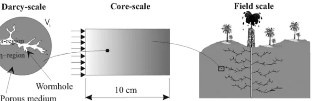
Figure 1 – The different scales of the problem.
respectivelyC∗
A̟ andV
∗
̟, are defined as follows.
C∗A̟ =CAβ
̟ ̟ = 1 V̟ V̟
CAβ d V (1)
V∗̟ =Vβ
̟ = 1 Vt V̟
Vβ d V (2)
Flow equation. For the flow description at this scale, a classical Darcy’s law has been obtained by averaging the Darcy-Brinkman formulation.
V∗β = − 1
µβ
K∗·∇Pβ∗−ρβg
(3)
∇ ·V∗β =0 (4)
where V∗
β and P
∗
β represent respectively the core-scale averaged velocity and
pressure andK∗ the core-scale permeability tensor. It must be pointed out that
this average velocity is linked to the two regional average velocitiesV̟∗ andV∗η, with the following relation:
Vβ∗ =V∗̟ +V∗η (5)
With regard to the transport and dissolution part, it was not obvious to apply an upscaling method which would lead to some core-scale equations valid in a general way. In fact, the value of the mass transfer coefficient appearing in the Darcy-scale model can strongly modify the acid transport behavior and the corresponding Darcy-scale dissolution pattern. Several approaches have been developed depending on whether the local mass equilibrium condition is verified or not.
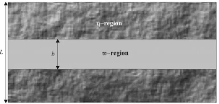
(̟−region) and the remaining porous matrix (η−region) are treated separately. The transport equations for the̟−region are written as
φ̟
∂C∗
A̟
∂t +V ∗
̟ · ∇C
∗
A̟ = ∇ ·
D∗∗̟·∇C∗A̟−α∗C∗A̟ (6)
∂φ̟
∂t = βs
ρσ
α∗C∗A̟ (7)
whereβs represents the stoichiometric coefficient of the reaction,ρσ the rock
density,α∗the core-scale mass transfer coefficient andφ
̟ the wormhole volume
fraction whereas the average concentration associated to theη−region,C∗Aη, is equal to 0.
Local mass non-equilibrium dissolution: One-equation model. In the more general case of local non-equilibrium conditions at the Darcy-scale, the more complex form of the local equations did not allow to directly infer the core-scale transport equation. Nevertheless, it was possible to propose a general form for the macroscopic transport-reaction equations within a one-equation model [6, 9], defined as follows:
ε∗β∂C ∗
Aβ
∂t +V ∗
β · ∇C
∗
Aβ = ∇ ·
D∗∗β ·∇C∗Aβ−α∗C∗Aβ (8)
∂εβ∗ ∂t =
βs
ρσ
α∗C∗Aβ (9)
whereε∗
β represents the core-scale porosity andC
∗
Aβ the average concentration
weighted by the porosity.
For instance, permeability is a function of porosity, or the mass transfer coeffi-cient depends on the cell Peclet number and porosity. Is it possible to use some similar relations at the core-scale?
In order to test such a possibility, rather than to solve numerically the closure problems with some non-representative boundary conditions, the dissolution pat-terns obtained at the Darcy-scale are used in this work to determine the effective coefficients. A series of Darcy-scale simulation is performed on a core of 25 cm length and 5 cm wide and used to obtain, by spatial integration, some core-scale effective parameters. We remind briefly in a first part the various results extracted from Darcy-scale simulations and presented in Golfier et al. [1]. Then, the definitions associated with the introduction of the core-scale parameters are presented and the possible independence of these coefficients with respect to the dissolution history is discussed based on the numerical experiments.
2 Darcy-scale numerical simulations
Different Darcy-scale simulations have been performed on a two-dimensional domain by varying the injection flow rateQ, the initial acid concentrationC0and the mass transfer coefficient valueα. Two principal results have been extracted from the model. First, the simulations allow to capture the different dissolution regimes, those corresponding to local equilibrium as well as those with non-equilibrium. We can see in Fig. 2 from Golfier et al. [1] an example of the dif-ferent dissolution figures obtained numerically for difdif-ferent acid injection rates. All these figures represent the porosity field. The obtained dissolution patterns are remarkably equivalent to the experimental dissolution patterns. These results were used to draw diagrams of the transitions between the different regimes.
Secondly, the performed simulations have confirmed the existence of an op-timum injection rate. This numerical optimum injection rate has been fitted with the experimental value through the proper choice of a single parameter,A, defining the mass transfer coefficient value through
αPecell, εβ
= Aα0
Pecell, εβ
(10)
(a) (b) (c) (d) (e)
0.4 0.5 0.6 0.7 0.8 0.9 1.0 Figure 2 – Porosity fields representative of the dissolution structure obtained numerically: Example of dissolution patterns: (a) face dissolution,Pe=8.32×10⁻⁴,Da=120; (b) conical wormhole,Pe=4.14×10⁻³% ,Da=24; (c) dominant wormhole,Pe=1.66, Da=6.01×10⁻²; (d) ramified wormhole,Pe=83.2,Da=1.2×10⁻³; (e) uniform dissolution,Pe=832,Da=1.2×10⁻⁴(Golfier et al.,J. Fluid Mech., 457, 2002).
as a function of the Peclet number, defined at the Darcy-scale Pecell, and the porosityεβ.
The calculations show that the optimum injection rate is linked with the Dam-köhler number value, calledDa1. Also, this model allowed to study the effect of many external parameters, such as the variation of temperature or concentration, or the use of other reacting fluids, like acids in emulsion, which give lower diffusion effects.
3 Macroscopic parameters and core-scale relations
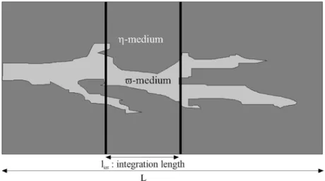
In this section, we discuss the determination of correlations between the dif-ferent core-scale effective coefficients from numerical experiments performed at the Darcy-scale. The definitions associated with these core-scale parameters are discussed below. We consider the domain represented in Fig. 1. Averaged properties, that could be used in a 1D core-scale representation are defined as follows. The different parameters of the problem (pressure, velocity, concen-tration...) are integrated on some interval of given length (Fig. 3) to provide
the core-scale properties, whose definitions have been given in Part I [2] and reminded in the introduction.
From the resulting porosity, pressure, velocity, and concentration fields, two additionnal core-scale parameters are calculated. From the pressure and veloc-ity fields, we calculate the head loss between two sections of the core. From the concentration field, we calculate the overall dissolution rate for a volume included between two cross sections. From these parameters it is possible to de-termine the core-scale permeability and the mass exchange coefficient. It must be emphasized that their definition is general, and does not depend on a particular model.
Figure 3 – Core-scale approach of the problem.
• Core-scale averaged permeability:
K∗ =µβ
∂P∗
β
∂x −1
V∗β
x (11)
• Core-scale averaged mass transfer coefficient:
α∗ = 1
C∗
Aβ
1
Vt
Vt
αCAβ d A (12)
history? In fact, as mentioned in the introduction, a direct relationship between the different macroscopic quantities may be historical, due to the coupling be-tween the flow velocity and the dissolution process. It must be emphasized that this question is of a general interest, and similar problems were found in geochemistry, or in dealing with dendritic mushy zones [7, 3]. This problem has been solved approximately at the Darcy-scale, where we have already de-termined the relations linking the different macroscopic properties, such as the permeability versus the porosity or the mass transfer coefficient as a function of the cell Peclet number and the porosity. We discuss below the application of the same ideas at the upper scale, by focusing particularly on the relationsK∗−φ
̟
andα∗= f (Pe, φ
̟, ...).
3.1 Macroscopic permeability relationship
We begin by representing the evolution of the core-scale permeabilityK∗ as a
function of the fluid fraction φ̟, or the core-scale porosity ε∗β, for the
disso-lution regimes: conical wormhole, wormholing and ramified wormhole. The reason for keeping the two parametersφ̟ andεβ∗ in the analysis have been
ex-plained in Part I [2]. In the case of local equilibrium, the Darcy-scale porosity remains constant in the non-dissolved areas. Thus, the single parameter charac-teristic of dissolution isφ̟. On the contrary, in the non-equilibrium cases, the
Darcy-scale porosity varies, and the two parametersφ̟ andε∗β characterize the
dissolution process, in a somehow independent manner.
For the two limit cases of dissolution,compact anduniform regime, the prob-lem simplifies to a 1D case and the dissolution front velocity is constant. It is remarkable to see that local equilibrium as well as non-equilibrium dissolution can lead to a stationary front displacement. Given the displacement velocity of the front is constant, theK∗−
φ̟ relation does not depend on the time evolution
3.1.1 Compact regime
For this regime, we have a sharp dissolution front with a displacement velocity Vqequal to
Vq = ρ V0C0
σεσ
β +C0
(13)
whereV0 andC0 are respectively the injection velocity and injection concen-tration.
The core-scale permeability fieldK∗is directly linked to the core-scale volume fractionφ̟, and their values depend on the position of the cross section versus
the dissolution front. We can write the relationshipK∗−φ
̟, for 0≤φ̟ ≤ 1,
under the form
K∗= K Kf lui d
(1−φ̟)Kf lui d +φ̟K
(14)
whereKf lui d represents the equivalent permeability of the fluid region.
3.1.2 Conical regime
Although the effective coefficients K∗
(t) and φ̟(t) are a function of time,
their evolutions, nevertheless, are not independent. Is it possible to obtain a relationship between these two parameters which is independent of the dissolu-tion history or does it stay a funcdissolu-tion of time?
Figure 4 – Schematic representation of tube dissolution.
the boundaries so that the flow may be considered steady (see Fig. 4). If we represent the wormhole by a tube of widthb, the effective permeabilityK∗can be estimated analytically. The equivalent permeability for the fluid zone is on the order ofb2/12 (in 2D) which leads, for the permeability K∗, to
K∗ = (1−φ̟)K0+φ̟b2/12
≈ φ̟b 2
12 for φ̟ >0
(15)
and the channel widthbcan be also expressed as a function of the fluid fraction, i.e. b=φ̟L. We obtain:
K∗= L 2φ3
̟
12 (16)
This relationship gives us an idea about theK∗−φ
̟ correlation existing in
our problem.
However, we are generally far from these theoretical conditions. We have represented in Fig. 5 the macroscopic permeability as a function of the fluid fraction atQ=1 cm3.h−1for different dissolution times. The integration interval is fixed atli nt = 0.75 cm. It is clear from these results that the permeability evolution remains a function of the time dissolution, except for small volume fractionsφ̟, and we have
K∗ = f(φ̟,t) (17)
This result can be physically explained from the dissolution figures. The closest we are from the inlet of the domain (i.e., the bigger the fluid fraction is), the less the wormhole can be represented by a tube in the studied section and, consequently, Eq. (16) is no longer verified.
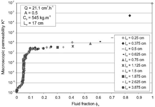
3.1.3 Wormholing regime
On the contrary, for the wormholing regime, the obtained results are closer to those predicted by the simplified theoretical model developed as indicated above. In fact, in this case, the wormhole geometry is similar to a tube. We have represented in Fig. 6, theK∗−φ
̟ relation for different injection rates, different
Figure 5 – Macroscopic permeability as a function of the fluid fraction (conical regime).
regime, a macroscopic relation quasi independent of the time evolution exists and can be expressed as
K∗ = f(φ̟) (18)
The influence of the integration length has also been investigated. Figure 7 shows theK∗−φ
̟ relationship, for various values ofli nt. This influence is
neg-ligible, as long as the interval length remains strictly smaller than the wormhole lengthLw.
Figure 7 – Effect of the variation of the integration interval length (wormholing regime).
3.1.4 Ramified regime
For the ramified regime, at last, Fig. 8 shows the permeability evolution as a function of the fluid fraction for different injection rates, different values of the mass transfer coefficient, and different times. It is obvious that aK∗−φ
̟
initial porous medium, and a transient zone with a porosity gradient due to the conditions of local non-equilibrium. The macroscopic permeabilityK∗can increase although the fluid fraction value is still 0 (cf. triangles in Fig. 8). Therefore,φ̟ does not seem to be convenient to correctly represent the
geo-metry of the domain. While our above discussion suggests that φ̟ and ε∗β
should be used independently, the results interpreted in terms of ε∗
β only lies
close to a single curve, Fig. 9. If confirmed, the core-scale relation could be written as follows
K∗= f ε∗β (19)
Figure 8 – Macroscopic permeability as a function of the fluid fraction (ramified regime).
The influence of the lengthli nt on the calculation ofK∗has also been verified and the simulations have confirmed that it was negligible provided it is strictly inferior to the wormhole length.
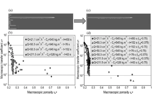
3.2 Macroscopic mass transfer relationship
The core-scale mass transfer coefficient α∗ seems more difficult to estimate.
Based on the relation at the Darcy-scaleα= f Pecell, εβ
Figure 9 – Macroscopic permeability as a function of the macroscopic porosity (ramified regime).
numberPeat the core-scale and the fluid fractionφ̟ (or the core-scale porosity
εβ∗for the local non-equilibrium dissolution regime). Moreover, we assume here that the dependence on the Peclet number is small compared with the depend-ence versusφ̟ (orε∗β). We will come back later on this assumption.
We have represented in Fig. 10 the evolution of the core-scale mass transfer coefficientα∗ into the core as a function of the core-scale porosityε∗
β for
dif-ferent dissolution times and difdif-ferent injection rates within theconical, worm-holingandramified regimes. This figure shows that the relationshipα∗−ε∗
β is
not as evident as the relationshipK∗−ε∗
β, although the plot is here in semi-log
scale. Even if a relationship seems to emerge in the case of the conical regime, we can remark the same phenomenon of instationarity observed for theK∗−ε∗
β
relationship. Atεβ∗ =0.2, initial porosity of the medium, we recover the mass transfer coefficient value at the Darcy-scale. When the fluid fraction (resp. the core-scale porosity) increases, the core-scale mass transfer coefficient decreases to pass by a plateau before going to 0 whenε∗
β → 1. The value depends on
the dissolution regime. In fact, ifα is proportional to 1/lβ2 wherelβ represents
propor-Figure 10 – Macroscopic mass transfer coefficient as a function of the macroscopic porosityε∗β.
tional to 1/l2
̟ wherel̟ is the wormhole width. Therefore, as the wormhole
width decreases from the conical regime to the wormholing regime, and from the wormholing regime to the ramified regime, although it is more difficult to define the limit of a wormhole in local non-equilibrium dissolution, the value of the core-scale parameterα∗decreases in the same way. Thus, when the macro-scopic porosityε∗
β increases, the core-scale mass transfer coefficient decreases
of a factorlβ/l̟
2
versus its initial value atεβ∗ =0.2.
The uncertainty about the relationship forα∗raises a major problem: like at
Figure 11 – (a) porosity field and (b)α∗−εβ∗correlation in wormholing regime before the dominant wormhole assumption; (c) porosity field and (d)α∗−ε∗β correlation in wormholing regime after the dominant wormhole assumption.
interest of using this assumption is confirmed by Fig. 11. The variation of the integration interval length has always a negligible influence on the correlation. An interesting parallel can be made between this assumption and the quasi-stationarity condition often used for solving the closure problems. With this last assumption, non-local effects in time and space are eliminated. In the same way, neglecting these wormholes allows to neglect the spatio-temporal varia-tions of the deviavaria-tions, and, consequently, the theory is valid only for some long times and far enough from the core inlet.
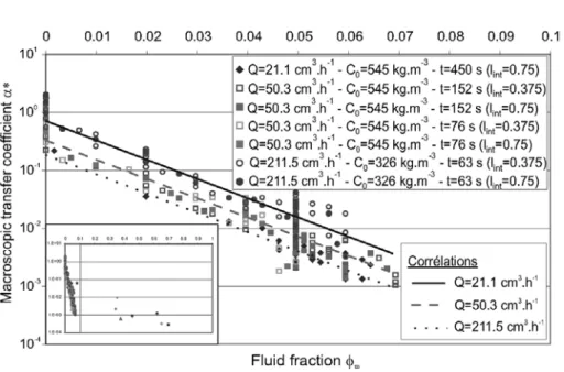
A zoom around the zone where the mass transfer coefficient strongly de-creases, and which contains the most important part of the dissolution physics, is represented in Fig. 12. This shows a non negligible dependence of the α∗
coefficient versus the injection velocity, i.e., the Peclet number. It is therefore necessary to take into account both the fluid fraction (or the porosityε∗
β)and
Figure 12 – Expression of correlationsα∗= f(Pe, φ̟) .
As a conclusion, several important results can be extracted from the develop-ment of these correlations:
• In theconical regime, effective coefficients cannot be uncoupled from the dissolution history.
• Simple correlations for the mass transfer coefficient remains difficult to be evaluated numerically. This represents an important problem for the development of a macroscopic model at the core-scale, while it is not clear at this point what is the impact of errors made in determining these correlations.
• The obtained correlations do not depend on the length of the integration intervalli nt, within the range of parameters explored.
4 Core-scale 1D model
these representations. The one-medium or one-equation local non-equilibrium model corresponds to the coupling between the flows equations, Eqs. (3) and (4), and the transport and dissolution equations, Eqs. (8) and (9). The devel-opment of thetwo-medium or two-equation local equilibrium model, based on the reaction-transport equations presented previously, Eqs. (6) and (7), needs the introduction of an additional assumption. In fact, this model requires the knowledge of the regional average velocities V∗
̟ andV
∗
η, i.e., solving of the
regional core-scale Darcy equations written as
∇ ·V∗̟ = 0 (20)
V∗̟ = − 1
µK ∗
̟ ·
∇P̟∗ −ρβg
in the̟ −phase (21)
and
∇ ·V∗
η = 0 (22)
V∗η = − 1
µK ∗
η·
∇Pη∗−ρβg
in theη−phase (23)
where K∗
̟ and K
∗
η represent the regional effective permeability tensors [8].
The two average velocities are linked with the following relation:
V∗β = V̟∗ +V∗η
= φ̟U̟∗ +(1−φ̟)U∗η
(24)
The intrinsic average velocity in the porous mediumU∗
ηbeing negligible
ver-sus the velocity in the fluid regionU∗
̟, we can assume
V∗
β ≈V
∗
̟ (25)
which allows us to use Eqs. (3) and (4) for the flow part. This approximation raises some difficulties only for some small values ofφ̟, when the wormhole
is not yet developed.
In this section, we test the capacity of these models to describe the core-scale dissolution physics. For this purpose, we compare the predictions given by the 1D averaged models with the simulations performed at the lower scale. Since the large-scale dispersion tensorD∗∗
201×101 nodes A=0.5
ρσ =2160kg.m−3 µ=1.10−3 Pa.s
ε∗
β =0.2
orφ̟ =10−4
β =1.62
D=2.10−9m.s−1 K∗=1.5·10−11m2 Table 1 – Numerical data for constant flow rate injection.
has not been calculated, it has been taken equal toφ̟D(orεβ∗Dfor local
non-equilibrium dissolution) in our simulations. This assumption has a small effect on the propagation time because we have focused here on thewormholingand
ramified regime, for which the Peclet number is relatively important. The Darcy-scale simulations which are used as reference, are obtained from the model described in Golfier et al. [1] and described briefly in Section 2. The local characteristics of the porous medium and its core-scale properties, including the initial values ofε∗
β(orφ̟) andK∗are given in Table 1. The correlations used for
the evolution of the mass transfer coefficientα∗ and the effective permeability
K∗are obtained as previously described.
Figure 13 – Comparison of the Darcy-scale model and the core-scale models forQ=21 cm3.h−1andC0=545 kg.m−3.
The comparison of our results for both models with Darcy-scale simulations are illustrated in Fig. 13 and 14 for Q = 21 cm3.h−1–C
Figure 14 – Comparison of the Darcy-scale model and the core-scale models forQ=50 cm3.h−1andC0=326 kg.m−3.
Q = 50 cm3.h−1 – C
0 = 326 kg.m−3, respectively. It must be emphasized here that the choice of the porosity threshold used to determine the tip of the wormhole is a decisive criterion: it has been fixed from the observation of the porosity fields at ε∗
β = 0.25 (φ̟ = 10−2 for the two-medium model). In the
case of the two-equation model, the initial value ofφ̟ att =0 s, theoretically
equal to 0, is fixed at 10−4for numerical reasons. The one-equation model does not succeed to correctly reproduce the propagation velocity of the wormhole and overestimates the breakthrough time in both regimes. The wormhole prop-agation, indeed, is represented in the one-equation model by an increase of ε∗
β
dom-inant wormhole assumption). This emphasizes the difficulty to express this coefficient independently of the history. The comparison of the fluid fraction fields obtained, either directly from the core-scale model, or by spatial integra-tion of the Darcy-scale porosity fields, confirms this assumpintegra-tion. One can see in Fig. 15, that theφ̟ value is correctly predicted, except for the inlet of the domain
where it is strongly underestimated because the core-scale model does not take into account the multitude of channels which propagate over a few centimeters.
Figure 15 – Fluid fraction values predicted by the Darcy-scale model and the core-scale 2-equation model forQ=50 cm3.h−1andC0=326 kg.m−3att =152 s.
These first results suggest that it is impossible to completely eliminate the
non-local effectsand that auniquecorrelation for the mass transfer coefficient,
independent of x and t, does not allow to perfectly reproduce the dissolution phenomenon at the core-scale. In the framework of the proposed core-scale models, several routes can be considered to model these mechanisms and correct the inaccuracy induced by such a representation: (i) taking into account the time effects by the introduction of a different α∗-correlation at short times such as
α∗ =α∗
α∗ =α∗
compact =constant forφ̟i nlet φ0. Then, theα
∗
compact variable becomes an additional parameter of the model that may be fitted to “experimental” data. The results of the introduction of this inlet compact dissolution model are illus-trated by the curve with the symbols (•) in Fig. 13 and 14 and the impact on the fluid fraction field is presented in Fig. 16.
Figure 16 – Fluid fraction values predicted by the core-scale 2-equation model with compact front forQ=50 cm3.h−1andC0=326 kg.m−3att =152 s.
These different results confirm that the description of the studied system by a two-medium domain may be an appropriate way for describing the dissolution phenomenon at the core-scale.
5 Conclusion
We have determined in this paper the correlations used for the effective coef-ficients which appear in the two core-scale transport-reaction models developed in Part I [2]. In both cases, the correlations have been directly extracted from the study of Darcy-scale numerical simulations and not from the solution of “closure problems”.
effective coefficients cannot completely be uncoupled from the non-local effects and the expressions of their correlations remainsnon-localfunctions, i.e., func-tions ofx and t. A good estimation of the mass transfer coefficientα∗ allows
however to correctly reproduce the wormhole propagation into the domain. What are the implications of these results for larger “averaging” volume, i.e., field scale problems? The introduction of a supplementary upscaling to de-scribe the wormholing phenomenon at the large-scale seems difficult. The use of our core-scale model as a near well-bore simulator coupled with a classical field model seems preferable. In fact, the results of our model could be used to calculate theskin effect factor in order to take into account the real conditions around the well within the field model. Therefore, we investigate at this time the ability of core-scale models to correctly reproduce the experimental results being based on accessible experimental data only, i.e., porosity and fluid fraction fields which can be obtained from tomography methods.
REFERENCES
[1] F. Golfier, C. Zarcone, B. Bazin, R. Lenormand, D. Lasseux and M. Quintard. On the ability of a Darcy-scale model to capture wormhole formation during the dissolution of a porous medium.J. Fluid Mech.,457(2002), 213–254.
[2] F. Golfier, B. Bazin, R. Lenormand and M. Quintard. Core-scale description of porous media dissolution during acid injection – part I: Theoretical development. Comp. Appl. Math.,
23(2-3) (2004), 173–194.
[3] B. Goyeau, T. Benihaddadene, D. Gobin and M. Quintard. Numerical calculation of the permeability in a dendritic mushy zone.Metall. and Mater. Trans. B,30B(1999), 613–622. [4] M.L. Hoefner and H.S. Fogler. Pore evolution and channel formation during flow and reaction
in porous media.AIChE J.,34(1) (1988), 45–54.
[5] C.M. Marle. Ecoulements monophasiques en milieu poreux.Rev. Inst. Français du Pétrole,
22(10) (1967), 1471–1509.
[6] C. Moyne, S. Didierjean, H.P. Amaral Souto and O.T. Da Silveira. Dispersion thermique en milieu poreux: Modèle à une équation. InCongrès Annuel de la Société Française des Thermiciens, pages 467–472. Elsevier, 1999.
[7] D.R. Poirier. Permeability for flow of interdentritic liquid in columnar-dentritic alloys.Met. Trans.,18B(1987), 245–255.
[8] M. Quintard and S. Whitaker. Transport in chemically and mechanically heterogeneous porous media – II. Large-scale mechanical equilibrium and the regional form of Darcy’s law.