ISSN 0101-8205 www.scielo.br/cam
A mixed nonlinear complementarity technique
for solving the dynamics of a dexterous
manipulation system
F.E. BUFFO and M.C. MACIEL
Department of Mathematics, Southern National University Av. Alem 1253, 8000 Bahía Blanca, Argentina Emails: [email protected] / [email protected]
Abstract. The versatility of a robot to perform a task is limited principally by the flexibility of its end-effector. In the last years, research has been focused on the development of a hand with several fingers since these devices are capable of manipulating and grasping objects of different forms. A dexterous manipulation system, composed of a robot hand with several fingers and
an object that will be held or manipulated, could be modeled as a set of rigid bodies in contact. The dynamics of several rigid bodies in contact tries to predict the accelerations and forces at the contact points of the set of rigid bodies with Coulomb friction. The calculation of such forces
allows us to determine if the contact is maintained or disappears and to plan a determined action. The equations that describe the problem form a system of differential algebraic equations. In this contribution the problem is reformulated as a mixed nonlinear complementarity problem (MNCP).
Then, an optimization problem with box constraints associated to the MNCP is presented using an adequate merit function. Conditions about the equivalence between the problems are established. Finally, the optimization problem is solved using a robust and efficient algorithm. Encouraging
numerical results are reported.
Mathematical subject classification: 49M37, 65C20, 90C30, 90C33.
Key words: linear complementarity problem, box constrained minimization, multi-rigid-body contact problem.
1 Introduction
Complementarity problems are of great importance in engineering applications because they are associated to the notion of equilibrium systems [4]. In the last decades, different types of complementarity problems have been studied: linear,
nonlinear, mixed, and efficient and robust algorithms have been developed to solve each of them.
This kind of problems arise in many engineering applications [4], such as mechanical contact problems, structural mechanics problems, structural design problems, nonlinear obstacle problems, elastohydrodynamics lubrication prob-lems, traffic equilibrium problems and optimum control probprob-lems, to mention some.
This work is organized as follows: section 2 presents generalities of the mixed nonlinear complementarity problem, and section 3 presents both the method for solving the MNCP via optimization, and existence and uniqueness results. Section 4, considers a dynamic model for several rigid bodies in contact, the equations that represent it [8, 9] and from these, the formulation of MNCP. In section 5 the numerical results for three-fingered hand manipulation system holding an object are reported. Finally, conclusions and future possibilities to continue on this research line are presented.
2 Mixed nonlinear complementarity problem
LetF :Rn→
Rnbe a vectorial function andLandCbe index sets that define a partition of{1,2, ...,n}. The problem of finding a vectorx ∈⊆Rnsuch that
FL(x)=0, xC ≥0, FC(x)≥0, xCtFC(x)=0, (1)
is called themixed nonlinear complementarity problem. The variablesxC are the complementarity variables and xLare the free variables that do not satisfy the complementarity and non negativity conditions.
The setis defined by
≡ {x ∈Rn :a≤ x ≤b},
whereaandbaren-dimensional vectors withai ∈ [−∞,∞)andbi ∈(ai,∞].
Ifxi is such thati ∈Lthenai = −∞andbi = ∞, while ifi ∈ Cthenai =0
ybi = ∞.
If the setL = ∅ and = Rn
+ = {x ∈ Rn : xi ≥ 0, i = 1, ...,n} then
we recover thenonlinear complementarity problem(NCP), if the functionF(x) is also affine then it is alinear complementarity problem(LCP). If the setC= ∅
it results in anonlinear system of equations.
A change in notation is considered, introducing a partition ofx, the vectors
u ∈ Rp, v ∈
and G : Rn → Rm. Slack variables z ∈ Rp are introduced, and the mixed
complementarity problem is expressed as follows,
u, z≥0, z−F(u, v)=0, utz=0, G(u, v)=0, (2)
whereu is the vector of complementarity variables and v is the vector of free variables, so that the dimension of the complementarity problem ism+2p.
The mixed nonlinear complementarity problem can be considered as a non-linear complementarity problem with an extra simultaneous nonnon-linear equa-tions system.
3 Solving of the complementarity problem via optimization
In order to reformulate the mixed complementarity problem as an optimization problem, it is necessary to introduce a merit function f :Rn×Rm×Rp→R.
The optimization problem that is solved is
(P)
min f(u, v,z)
s.t
u≥0, z ≥0.
(3)
The advantage of reformulating the MNCP using the aforementioned strategy is the possibility of applying efficient algorithms and theoretical results known for optimization problems. In general, the algorithms used to solve optimization problems obtain stationary points, that is, points that only satisfy the first order optimality conditions. The convergence to a global minimum can be guaranteed if the merit function is convex.
Optimization problems have been extensively studied in recent years and many efficient algorithms exist to find the solutions. To obtain a solution to the mixed nonlinear complementarity problem (3) with the merit function,
f(u, v,z)= F(u, v)−z 2+ G(u, v) 2+(utz)2 , (4) Andreani, Friedlander, Mello and Santos [1] establish conditions that allow us to assure that stationary points of (3) with the merit function (4) are also global minimizers and solutions of the MNCP.
4 Mathematical model of the contact problem
The dynamic system is formed by a determined number of passive bodies
called objects and a given number ofactive bodies called manipulators. The first ones move in response to external and contact forces. The hypotheses of the proposed model [7, 8] are:
1. The bodies are rigid. There are no constraints on the shape of the bodies.
2. The normal direction at each contact point is well-defined, this means that the surface of the passive body has a tangent plane on each contact point.
3. There exists friction at each contact point. A friction model and a friction law must be selected.
4. The manipulator is formed bylinksandjoints; the manipulator joints do not form closed loops. Each joint has only one degree of freedom. All allowed contacts are unilateral.
5. All links are connected to a grounded link (reference coordinate).
The equations and constraints that govern the model are: the Newton-Euler movement equations, for the objects and manipulators, the unilateral and bi-lateral kinematic constraints due to the contact, the dynamic conditions of the contact, that is the non interpenetration principle and non tensile forces, and the friction law of the contact.
To develop the equations that govern the dynamics of the set of rigid bodies in contact, it is considered that in a certain instantt0certain number of objects,
nobj, are in contact among them and with a certain number of manipulators, nman, beingncthe total number of contacts.
Letci jdenote the contact force acting on the bodyithrough contactjexpressed
in the contact frame Cj, with normal, tangential and orthogonal components (ci j)n,(ci j)t and(ci j)o. The sum of the forces acting on the bodyi is equal to
the mass times the acceleration of its mass center and it is expressed as
j∈Bi
Wi jci j +gobj,i+hobj,i = Mobj,iq¨obj,i, (5)
whereBi is the set of indices of the points of contact of the bodyi,gobj,i ∈ R6
is the external generalized force (expressed in the fixed reference coordinates of the bodyBi), which acts upon it,hobj,i ∈ R6is the term of movement quantity,
¨
of the object, Mobj,i ∈ R6×6 is the symmetric positive definite mass matrix of
the objectipartitioned as:
Mobj,i =
M1,i 0
0 M2,i
, (6)
with M1,i =mobj,i I3,I3being the identity matrix, andM2,i the bodie’s inertial
tensoriexpressed in the baseBi. The matrixWi j ∈R6×3transforms the contact
forcesci j into a generalized force,Fi j. Thewrench matrices Wi j contain all the
geometric information about contact j.
The previous equations extended to all objects, express the contact forces by components, and the following matrix equation is obtained:
Wncn+Wtct +Woco+gobj+hobj = Mobjq¨obj, (7)
with cα ∈ Rnc,Wα ∈ R6nobj×nc, α ∈ {n,t,o}, the vectors gobj, hobj, q¨obj ∈ R6nobj, andM
obj ∈R6nobj×6nobj is
Mobj = diag{Mobj,1,Mobj,2, ...,Mobj,nobj}. (8)
The dynamics equations for the manipulators are obtained likewise:
τ −(Jntcn+Jttct +Jotco+gman+hman) = Mmanθ¨man, (9)
where, if we call nθ the number of manipulator joints, θ˙man ∈Rnθ is the
velo-city of the joints,τ ∈ Rnθ is the vector of joint effort, J
n, Jt and Jo ∈ Rnθ×nc
are the Jacobian matrices which determine the effect of the α-th component of the force (ci j)α over the componentα of the vector of joint effortτ, with α ∈ {n,t,o}, Mman ∈ Rnθ×nθ is the symmetric positive definite inertia matrix, gman(θman)∈Rnθ is the vector of torques induced by gravity,hman(θman,θ˙man)∈ Rnθ represents the vector of torques and forces induced by Coriolis and
centri-petal accelerations andθ¨man ∈Rnθ is the vector of joint accelerations.
The motion of each object in contact is subject to kinematic constraints:
vα =Wαtq˙obj−Jαθ˙man, α∈ {n,t,o}, (10)
aα =Wαtq¨obj−Jαθ¨man+ ˙Wαtq˙obj− ˙Jαθ˙man, α ∈ {n,t,o}. (11)
wherevα ∈ Rnc is the linear velocity andaα ∈ Rnc is the linear acceleration in the directionα, expressed in the contact frameCj,q˙objandθ˙manare the vectors
In each contact point jthe normal component of the velocity is zero,
vj n =0, j =1, ...,nc. (12)
Among thenccontact points,nRdenotes the number of rolling contacts andnS denotes the number of sliding contacts, so thatnc =nS+nR. SandRdenote the sets of respective indices.
A rolling contact point is characterized by the fact that both the tangential and orthogonal components of the velocity at such point are zero, that is
vj t =vj o=0, j ∈R, (13)
and a sliding contact point is characterized by the fact that the tangential or orthogonal components of the velocity at such point is different from zero,
vj t =0 o´ vj o =0, j ∈S. (14)
To avoid interpenetration, the motion of the object is subject to the constraint known asnon penetration principle of Signorini,
an≥0. (15)
The forces on the contact point must have non negative normal components, this means that they are not tensile,
cj n ≥0, j =1, ...,nc. (16)
For any contact point j, if(an)j =0 the contact is maintained and(cn)j ≥0,
whereas if(an)j >0 the contact disappears (breaking) and(cn)j =0.
Considering (15) and (16) relating the accelerations and the forces of the con-tact points, the complementarity constraint is established,
atncn=0. (17)
To grasp an object, friction forces are required and so a friction model must be established. The choice of the friction model determines the form of the matrices Wα which appear in the equation (7) and the matrices Jα in equation (9) withα ∈ {n,t,o}. The law used here is theCoulomb friction law which establishes that the contact force on the point jfalls within or on the boundary of the corresponding friction cone, represented as follows:
whereµj is the friction coefficient on the contact point j.
If the contact is sliding, the contact force must lie on the border of the friction cone with its friction component directly opposed to the sliding velocity and satisfy
µjcj nvjα+cjα
v2j t +v2j o =0, j∈S, α ∈ {t,o}. (19) If the contact is rolling, the contact force can have some direction and magni-tude, within the cone defined by (16) and (18) and satisfy
µjcj najα +cjα
a2
j t +a2j o=0, j ∈R, α ∈ {t,o}. (20)
Equation (19) differs significatively from equation (20), since the former is linear in the unknownscj nandcjα because the velocities are data, whereas the latter is nonlinear because the accelerations are unknowns.
Considering that in the initial instant t0 qobj, q˙obj, gobj, hobj, Mobj are
known for the objects;θman, θ˙man, τ, gman, hman, Mmanfor the manipulators;
the torque matricesW and the Jacobian matrices Jman,q˙obj andθ˙mansatisfying
the kinematic constraints (10), (12) and (13), to solve the dynamics of several bodies in contact means to determineq¨obj, θ¨man,cn, ct, co, an, at, ao,which
satisfy the equations (7), (9), (11), (15), (17), (19) and (20).
Since the algebraic-differential equation system that results is complex to solve, it is convenient to reformulate it as a mixed nonlinear complementar-ity problem. Thus, a discretization of the independent variable is considered, assuming that in the instant t0 an initial configuration, i.e. a contact and the position and velocities of all the bodies is known. Therefore, to establish the configuration in an instantt0+t, a complementarity problem is solved. This implies analyzing whether the contact is maintained or not, and calculating the positions and velocities of the new configuration.
Taking into account that the inverses ofMobjandMmanexist,q¨objandθ¨mancan
be obtained from the equations (7) and (9). Replacingq¨objandθ¨manin equation
(11) and defining aα ∈ Rnc, with α ∈ {n,t,o}, a linear equation system is obtained
an at ao
= A
cn ct co
+
bn bt bo
, (21)
A =
Ann Ant Ano At n At t At o Aon Aot Aoo
= J
t
where the Aαγ are submatrices of Awhich consist of rows and columns corre-sponding to the directionsαandγ respectively, withα, γ ∈ {n,t,o}.
FromMobj, Mman,Wn,Wt,Wo,Jnt, Jtt, y Jot, the matrices
M =
Mobj
−1
0
0 Mman
−1
, J =
Wn Wt Wo Jnt Jtt Jot
, (23)
and the vector
bn bt bo
= ˙J
t
˙ qobj − ˙θman
+ JtM
gobj+hobj gman+hman−τ
. (24)
are defined.
Equation (19) is solved to obtaincj t andcj o with j ∈ Sand replace them in
(21). The acceleration vectors and contact forces are partitioned for the contacts
RandS. Since there are no additional constraints for the tangential and orthog-onal components of the accelerations on the sliding contact points, the equations of the system (21) which define these components can be set apart without af-fecting the solution of the complementarity problem
aSn aRn aRt aRo
= ˜A
cSn cRn cRt cRo
+
bSn bRn bRt bRo
, (25)
where:
˜ A =
(A˜nn)SS (Ann)SR (Ant)SR (Ano)SR
(A˜nn)RS (Ann)RR (Ant)RR (Ano)RR
(A˜t n)RS (At n)RR (At t)RR (At o)RR
(A˜on)RS (Aon)RR (Aot)RR (Aoo)RR
, (26)
(A˜nn)SS
(A˜nn)RS
(A˜t n)RS
(A˜on)RS
≡
(Ann)SS
(Ann)RS
(At n)RS
(Aon)RS
−
(Ant)SS
(Ant)RS
(At t)RS
(Aot)RS
VtS −
(Ano)SS
(Ano)RS
(At o)RS
(Aoo)RS
VoS, (27)
VαS = diag
µj vjα
v2j t +v2j o
Equations (15–17), (18–20), (25–28), constitute a mixed nonlinear comple-mentarity problem as defined in (1) associated to the 3D dynamics of several rigid bodies in contact with Coulomb friction.
To express the mixed nonlinear complementarity problem with the notation used in (2), the slack variablessj are introduced by
sj =µ2jc 2
j n−c 2 j t −c
2
j o≥0, j ∈R, (29)
and the vector of complementarity variablesλwhose components are given by
λj =
a2j t +a2j o, j∈R. (30) Vector u ∈ RnS+2nR corresponds to the complementarity variables, vector v ∈ R4nR corresponds to the free variables and the vector of slack variables z ∈RnS+2nR are defined
u =
cSn cRn λ
≥0, v=
cRt cRo aRt aRo
, z =
aSn aRn s
≥0. (31)
Partitioning adequately the system (25) and from (29), the following vectorial functionF :RnS+6nR →RnS+2nR is obtained,
F(u, v)=
A1 A2
cSn cRn cRt cRo
+
bSn bRn
s(cRn,cRt,cRo)
, (32)
with
A1=
(A˜nn)SS (Ann)SR
(A˜nn)RS (Ann)RR
, A2=
(Ant)SR (Ano)SR
(Ant)RR (Ano)RR
.
The vectorial functionG :RnS+6nR →R4nR is expressed as follows
G(u, v)=
G1(u, v)
G2(u, v)
G3(u, v)
, (33)
where
(G2(u, v))j =µjcj naj o+cj oλj, j ∈R, (35)
G3(u, v)=
aRt aRo
− A3 A4
cSn cRn cRt cRo
−
bRt bRo
, (36)
A3=
(A˜t n)RS (At n)RR
(A˜on)RS (Aon)RR
, A4=
(At t)RR (At o)RR
(Aot)RR (Aoo)RR
.
5 Numerical results
In this section, we show how the mixed non linear complementarity technique presented in the previous sections is used. Let us consider the model of an object grasped by a robot hand with three fingers.
The initial configurationfor the proposed example is established fixing the location of the coordinate systems with origins in the mass center of the body (B), the base of the j-th robot (Sj), the j-th point of contact (Cj) and the palm
of the hand (P). The origin of the reference coordinate system is located in the palm of the robot hand. Figure 1 presents a bidimensional scheme for the given configuration.
-0.4
-0.2
0.
0.2
0.4
-0.2
0.
0.2
0.4
. . . . . . . . . . . . . . . . . . . . . . . . . . . . . . . . . . . . . . . . . . . . . . . . . . . . . . . . . . . . . . . . . . . . . . . . . . . . . . . . . . . . . . . . . . . . . . . . . . . . . . . . . . . . . . . . . . . . . . . . . . . . . . . . . . . . . . . . . . . . . . . . . . . . . . . . . . . . . . . . . . . . . . . ... ... . . . . . . . . . . . . . . . . . . . . . . . . . . . . . . . . . . . . . . . . . . . . . . . . . . . . . . . . . . . . . . . . . . . . . . . . . . . . . . . . . . . . . . . . . . . . . . . . . . . . . . . . . . . . . . . . . . . . . . . . . . . . . . . . . . . . . . . . . . . . . . . . . . . . . . . . . . . . . . . . . . . . . . . . . . . . . . . . . . . . . . . . . . . . . . . . . . . . . . . . . . . . . . . . . . . . . . . . . . . . . . . . . . . . . . . . . . . . . . . . . . . . . . . . . . . . . . . . . . . . . . . . . . . . . . . . . . . . . . . . . . . . .•
S
2 . . . . . . . . . . . . . . . . . . . . . . . . . . . . . . . . . . . . . . . . . . . . . . . . . . . . . . . ... . . . . . . . . . . . . . . . .−
x
. . . . . . . . . . . . . . . . . . . . . . . . . . . . . . . . . . . . . . . . . . . . . . . . . . ... ...−
y
•
S
1 . . . . . . . . . . . . . . . . . . . . . . . . . . . . . . . . . . . . . . . . . . . . . . . . . . . . . . . . . . ... . . . . . . . . . . . . . . . .−
x
. ... . . . .y
•
S
3 . . . . . . . . . . . . . . . . . . . . . . . . . . . . . . . . . . . . . . . . . . . . . . . . . . . . . . . . . . . . . . . . . . . . . . . . . ...x
. ... . . . .y
. ... ... ... ... ... . ... . . ... ... ... ... ... . . . . . . . . . . . . . . . . . . . . . . . . . . . . . . . . . . . . . . . . . . . . . . . . . . . . . . . . . . . . . . . . . . . . . . . . . . . . . . . . . . . . . . . . . . . . . . . . . . . . . . . . . . . . . . . . . . . . . . . . . . . . . . . . . . . . . . . . . . . . . . . . . . . . . . . . . . . . . . . . . . . . . . . . . . . . . . . . . . . . . . . . . . . . . . . . . . . . . . . . . . . . . . . . . . . . . . . . . . . . . . . . . . . . . . . . . . . . . . . . . . . . . . . . . . . . . . . . . . . . . . . . . . . . . . . . .•
C
2•
C
1•
C
3B
•
...y
. . . . . . . . . . . . . . . . . . . . . . . . . . . . . . . . . ...x
Using algorithm 1, the system configuration of various bodies in contact in the instantt0+tfrom an initial configuration is obtained.
Algorithm 1. Givenµ, nR, nS, and the configuration parameters,
1. Define the initial configuration.
1.1. Calculate the coordinate transformation matrices,
1.2. Calculate the vector of positions of the manipulator joints, θman (Problem of inverse kinetics).
2. Calculate the matrices for the object W , Mobj.
3. Calculate the manipulator matrices, Jman, Mman.
4. Calculate the matrices of the complementarity problem,M,J, andA.˜
5. Solve the complementarity problem via optimization.
6. Define the new configuration.
In step 5, the optimization problem can be solved by any appropriate algorithm. To establish the initial configuration, the matrices pt and pt t ∈ R3×nc are
considered. Each column of pt, pt(., j)contains the j-th point of contact with
respect to the systemP; while the j-th column of pt t contains the coordinates
of the j-th point of contact with respect to the coordinate system Sj. For the
proposed configuration, the matrices are,
pt =
r cos(σ ) r cos(σ ) −r −r si n(σ ) r si n(σ ) 0
acm acm acm
,
pt t =
−(b˜−r)cos(σ ) −(b˜−r)cos(σ ) b˜−r
(b˜−r)si n(σ ) −(b˜−r)si n(σ ) 0
acm acm acm
,
whereris the sphere radius,acmestablishes the location of the sphere mass center
with respect to the coordinate axes system of the palmP, pcm =(0,0,acm),b˜
Bwith the points of contactC1and/orC2. As observed in figure 1, the location
of the contactsC1andC2is symmetric respect toB.
The rotation matrices for each contact have the following expressions:
RP,C1 = Qz(−σ )Qy
−
π 2
, RP,C2 = Qx
π 2
Qz(−σ ),
RP,C3 = Qz
π
2
Qx
π
2
,
whereQα(ϕ)are the matrices representing elemental rotation around the direc-tionα, with an angleϕ.
Thefriction modelis characterized by the matrix,
Bf =
1 0 0
0 1 0
0 0 1
0 0 0
0 0 0
0 0 0
. (37)
The matrixW ∈R6×9is expressed as follows, W =
W1Bf W2Bf W3Bf
, (38)
withWj, with j =1,2,3, defined as,
Wj =
RP,Cj 0
ˆ
pt(.,j)RP,Cj RP,Cj
. (39)
The following notation is used: given any vectorv∈R3,vˆ ∈R3×3we define
ˆ
v=
0 −v3 v2
v3 0 −v1
−v2 v1 0
. (40)
The inertia matrix of the sphere respect to the mass center is M2 = 2 5mr
2I3,
The mass matrix of the objectMobj ∈R6×6is,
Mobj =
m I3 0
0 M2(P)
. (41)
The experiments were performed using a well known robot PUMA (Pro-grammable Universal Manipulator for Assembly). For each manipulator the Jacobian matricesJfjand the mass matricesMfj are calculated using therobotic toolbox in MATLAB[2]. The Jacobian matrix for all the three fingered hands
Jman∈R9×nθ results
Jman =
J1 0 0
0 J2 0
0 0 J3
, (42)
with
Jj = Btf
Rt
P,Cj R t
P,Cjpˆ t t t(.,j)
0 Rt
P,Cj
Jfj,
whereBf is the matrix of the friction model.
The inertia matrix of the manipulatorMfj ∈R
nθj×nθj is
Mfj(θ )= nθ
j=1
JLtj(θ )MLjJLj(θ ), (43)
whereJLjandMLj are the Jacobian matrices and the generalized inertia matrices
of the linkLj. The mass matrix of the three fingersMman∈Rnθ×nθ is
Mman=
Mf1 0 0
0 Mf2 0
0 0 Mf3
. (44)
If it is considered that all the contacts are sliding, the MNCP is reduced to a LCP. Solving the LCP means solving the optimization problem defined in (3) with the merit function
f(cn,an)= an− ˜Anncn−bn 2 2 + (a
t
ncn)2, (45)
where the vectorbn ∈R3is obtained from equation (24), ˜
The matrices Vt and Vo are defined in (28) and each submatrix Aαγ has the expression
Aαγ =Wαt(Mobj)−1Wγ +Jα(Mman)−1Jγt. (47) A variable change is performed,tˆ∈R6,tˆ=[c
n,an]t so that the merit function
is expressed as follows,
f(tˆ)= 3
i=1
tˆi+3 − 3
j=1
Mi jtˆj − (bn)i
2 +
3
i=1 ˆ titˆi+3
2
. (48)
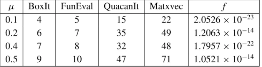
The matrixMin the complementarity problem depends on the friction coeffi-cients on the contact points. For the proposed example, and using a PUMA560 manipulator the results obtained are:
µ BoxIt FunEval QuacanIt Matxvec f
0.1 4 5 15 22 2.0526×10⁻²³
0.2 6 7 35 49 1.2063×10⁻¹⁴
0.4 7 8 32 48 1.7957×10⁻²²
0.5 9 10 47 71 1.0521×10⁻¹⁴
Table 1 – Results of the optimization problem for the LCP.
µ cn1 cn2 cn3 an1 an2 an3
0.1 2.2867 2.7800 3.8067 0. 0. 0.
0.2 1.4669 2.2680 2.7108 0. 0. 0.
0.4 3.3672 6.3354 6.5843 0. 0. 0.
0.5 14.745 29.731 28.862 0. 0. 0.
Table 2 – Results of the LCP for the sliding contacts.
As can be observed in Table 2, the contact is mantained in all cases. If it is considered that the three contacts are rolling, the problem is formulated as a MNCP. The MNCP is solved considering the equivalent optimization problem (3), using the merit function proposed in (4). The following variable change is performedt˜ =
cn, ct, co, an, at, ao, s , λ
t
, with the merit function
µ x0 BoxIt FunEval QuacanIt Matxvec f
0.1 0 30 42 1179 1561 3.9561×10⁻¹⁰
0.2 0 21 35 979 1390 1.4722×10⁻¹⁵
0.4 0 18 30 762 1109 9.5039×10⁻¹⁶
0.6 0 15 25 625 934 6.7051×10⁻¹²
0.8 0 27 38 1021 1411 6.4478×10⁻¹¹
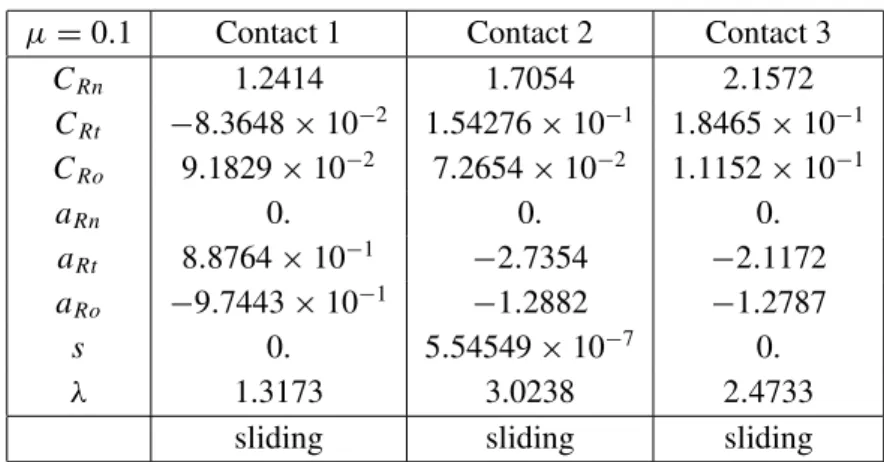
Table 3 – Results of the optimization problem for the MNCP.
µ=0.1 Contact 1 Contact 2 Contact 3
CRn 1.2414 1.7054 2.1572
CRt −8.3648×10⁻² 1.54276×10⁻¹ 1.8465×10⁻¹ CRo 9.1829×10⁻² 7.2654×10⁻² 1.1152×10⁻¹
aRn 0. 0. 0.
aRt 8.8764×10⁻¹ −2.7354 −2.1172 aRo −9.7443×10⁻¹ −1.2882 −1.2787
s 0. 5.54549×10⁻⁷ 0.
λ 1.3173 3.0238 2.4733
sliding sliding sliding
Table 4 – Results of the MNCP for the rolling contacts.
where
sum1 = 3
j=1
˜
t(j+18)−(µ(j)t˜(j))2+(t˜(j+3))2+(t˜(j+6))2 2
,
sum2 = 3
j=1
µ(j)t˜(j)t˜(j+12)+ ˜t(j+3)t˜(j+21) 2
+ µ(j)t˜(j)t˜(j+15)+ ˜t(j+6)t˜(j+21)
2
,
sum3 = 3
j=1 ˜
t(j)t˜(j+9)+ 3
j=1 ˜
t(j+18)t˜(j+21),
The optimization problem solved is of dimension 24. It has been solved by using a robust and efficient algorithm developed by Friedlander and Martínez [5, 6]. The results obtained are summarized in tables 3 and 4.
6 Conclusions and future research
The dynamics of several rigid bodies in contact with Coulomb friction is pre-sented as a MNCP. The complementarity problem is reformulated as a box constraints optimization problem.
It is worth noting that the optimization problem for the mixed case is general. Contrary to many methods which are specific to linear or nonlinear complemen-tarity problems, this technique can be applied to any of them by only defining appropriately the merit function and the box.
An example of a robot hand with three fingers grasping an object is considered. Matrices of smaller dimensions, which respond to a real model, were preferred over those with greater dimensions. Functions inMATLABwere developed to obtain the system matrices and the optimization problem with box constraints was solved using theeasycomputing program. The robustness of the optimiza-tion method we used, allowed us to obtain a soluoptimiza-tion in most cases. In the future, we wish to generate contact problems with a greater number of bodies and points of contact, both rolling and sliding, trying to consider the structure of the matrices which are generated without losing sight of the physical meaning. Furthermore, it is considered of interest to complete the kinematics and dynamics calculation of the robot problem for a sequence of times t1, t2, t3... and to verify if the obtained results are satisfactory. We plan to continue deepening the study of the MNCP in general following the proposed research line.
Acknowledgments. The authors gratefully acknowledge suggestions and comments of the referee.
This work was partially supported by the Universidad Nacional del Sur, Pro-ject 24/L057 and Fundacion Antorchas, Proyect 13900-4.
REFERENCES
[1] R. Andreani, A. Friedlander, M.P. Mello and S.A. Santos, Mixed nonlinear complementarity problems via nonlinear optimization: numerical results on multi-rigid-body contact problem with friction, 2003. To appear in International Journal of Computational Engineering Science.
[2] P.I Corke,Robotics TOOLBOX for MATLAB (Release 6). Available at http://www.cat.csiro.au/ cmst/satff/pic/robot (2001).
[4] M.C. Ferris and J.S. Pang, Engineering and economic applications of complementarity prob-lems.SIAM Review,39(4) (1997), 669–713.
[5] A. Friedlander and J.M. Martínez, On the maximization of a concave quadratic function with box contraints.SIAM Journal on Optimization,4(1994), 177–192.
[6] A. Friedlander, J.M. Martínez and S.A. Santos, On the resolution of large scale linearly constrained convex minimization problems. SIAM Journal on Optimization, 4 (1994), 331–339.
[7] R.M. Murray, Z. Li and S.S. Sastry,A Mathematical Introduction to Robotic Manipulation. CRC Press, 2000 Corporate Blvd., N.W., Boca Raton, Florida (1994).
[8] J.S. Pang and J.C. Trinkle, Complementarity formulations and existence of solutions of multi-rigid-body contact problems with coulomb friction. Mathematical Programming, 73(1996), 199–226.