Measurements and modelling of molecular iodine emissions, transport and photodestruction in the coastal region around Roscoff

(1)

ACPD

9, 21165–21198, 2009

I₂ emission modelling and measurements

R. J. Leigh et al.

Title Page

Abstract Introduction

Conclusions References

Tables Figures

◭ ◮

Back Close

Full Screen / Esc

Printer-friendly Version

Interactive Discussion Atmos. Chem. Phys. Discuss., 9, 21165–21198, 2009

www.atmos-chem-phys-discuss.net/9/21165/2009/ © Author(s) 2009. This work is distributed under the Creative Commons Attribution 3.0 License.

Atmospheric Chemistry and Physics Discussions

This discussion paper is/has been under review for the journalAtmospheric Chemistry and Physics (ACP). Please refer to the corresponding final paper inACPif available.

Measurements and modelling of

molecular iodine emissions, transport

and photodestruction in the coastal

region around Rosco

_ff

R. J. Leigh1, S. M. Ball2, J. Whitehead4, C. Leblanc5, A. J. L. Shillings3, A. S. Mahajan6, H. Oetjen6, J. R. Dorsey4, M. Gallagher4, R. L. Jones3, J. M. C. Plane6, P. Potin5, and G. McFiggans4

1

Department of Physics and Astronomy, University of Leicester, Leicester, UK.

2

Department of Chemistry,University of Leicester, Leicester, UK

3

Department of Chemistry, University of Cambridge, Cambridge, UK

4

School of Earth, Atmospheric and Environmental Sciences, University of Manchester, Manchester, UK

5

(2)

ACPD

9, 21165–21198, 2009

R. J. Leigh et al.

Title Page

Tables Figures

◭ ◮

Back Close

Full Screen / Esc

Interactive Discussion

6

School of Chemistry, University of Leeds, Leeds, UK

Received: 11 September 2009 – Accepted: 12 September 2009 – Published: 7 October 2009

Correspondence to: R. J. Leigh (r.j.leigh@leicester.ac.uk)

(3)

ACPD

9, 21165–21198, 2009

R. J. Leigh et al.

Title Page

Tables Figures

◭ ◮

Back Close

Full Screen / Esc

Abstract

Emissions from the dominant six macroalgal species in the coastal regions around Rosccoff, France, have been modelled to support the Reactive Halogens in the Marine Boundary Layer Experiment (RHaMBLE) campaign undertaken in September 2006. A 2-D model was used to explore the relationship between point and line

measure-5

ments of molecular iodine concentrations, and total regional emissions, based on sea-weed I₂ emission rates measured in the laboratory. The relatively simple modelling technique has produced modelled point and line data, which compare quantitatively with campaign measurements, and provide a link between emission fields and the different measurement geometries used to quantify atmospheric I₂concentrations

dur-10

ing RHaMBLE. During nightime, absolute concentrations in the region of 5 pptv are predicted and measured in the LP-DOAS measurements, with site concentrations pre-dicted and measured up to 40 pptv, compatible with concentrations above Laminariales beds of approximately 2.5 ppbv. Daytime measured concentrations of I₂ at site corre-late with modelled production and transport processes, however complete recycling of

15

photodissociated I2is required in the model to quantitatively match measured

concen-trations. Additional local source terms are suggested to provide a feasible mechanism to account for this discrepancy.Total of I2 emissions over the 100 km

2

region around Roscoffare calculated as 1.5×1019molecules per second during the lowest tides.

1 Introduction

20

Most techniques for atmospheric composition measurement provide a single point sample, from which conclusions are sought over a given region or scenario. Tech-niques such as long-path differential optical absorption spectroscopy (LP-DOAS) pro-vide integrated measurements along a folded line of site between a light source and retro-reflector. In many cases, a relatively simple model can significantly improve

un-25

derstanding of the relationship between point and line data, and temporally varying

(4)

ACPD

9, 21165–21198, 2009

R. J. Leigh et al.

Title Page

Tables Figures

◭ ◮

Back Close

Full Screen / Esc

Interactive Discussion and spatially inhomogeneous concentrations in a region around the monitoring site.

Results are presented here from a model of molecular iodine emissions produced in support of the RHaMBLE campaign hosted at the Station Biologique de Roscoff(SBR) (McFiggans et al., 2009). This model is used to place novel measurements of I2 from

a broad-band cavity ring down system (BBCRDS) and a LP-DOAS instrument into a

5

regional context.

2 The model

The model incorporates two horizontal spatial scales and a temporal domain, with a vertical component included in footprint modelling calculations. The horizontal grid consists of 746 by 227 elements, each of 0.0005×0.0005 degrees extending from

10

−4.2075 to −3.835 degrees longitude, and 48.6725 to 48.7855 degrees latitude. In the Roscoffregion, this resolution corresponds to grid boxes of approximately 36.7 m longitudinally by 55.6 m latitudinally. Bathymetry and macroalgal distribution informa-tion was mapped on to this model grid. Tide and meterological data was applied to this spatial information at 1-min resolution from 5 to 28 September 2006.

15

2.1 Seaweed speciation and site bathymetry

The Roscoffinter-tidal zone in front of the SBR extends more than five kilometers in length and about 1 km in width. This very shallow inter-tidal zone at Roscoff means that the waters closest to the shoreline are too shallow for Laminariales species, so al-though a larger horizontal surface area of seaweed beds becomes exposed at low tide

20

in the vicinity of the SBR, this mainly consists of fucoids. The distribution of seaweed species is rather patchy in the inter-tidal zone and is mainly dominated byFucus spp.

and Ascophyllum beds, however there is also a small amount of Laminaria digitata,

Saccharina latissimaandLaminaria ochroleucain the channel and tide pools between the site and the island Ile de Batz. The south shore of Ile de Batz includes sheltered

(5)

ACPD

9, 21165–21198, 2009

R. J. Leigh et al.

Title Page

Tables Figures

◭ ◮

Back Close

Full Screen / Esc

Interactive Discussion shallow patchy habitats with sand and gravel which surround rocky areas covered by

fucoids except when exposed to strong tide currents. L.(mainlyhyperborea) beds ex-tend to the north of Ile de Batz, whereasL. digitataflourishes in moderately exposed areas or at sites with strong water currents in the western part of the study site (Ile de Batz and islets from Perharidy) and north-east from the Ile de Batz. It also occurs in

5

rockpools up to mid-tide level and higher on wave-exposed coasts of the Ile de Batz. The vertical zonation of various species of seaweed is very distinct on rocky shores with each species often forming a belt at a certain elevation in the eulittoral zone (the area between the highest and the lowest tides) and also in the subtidal zone (the area extending below the zero of the marine charts). It is thought that the driving force of this

10

zonation is a combination of biotic factors and the tolerance of the different species to abiotic factors such as temperature, light, salinity, dehydration, and mechanical forces caused by wave action (L ¨uning, 1990). A typical kelp bed from the Roscoffregion is shown in Fig. 2. In the North Atlantic, exemplified in the study site in front of the SBR, the eulittoral zone in sheltered habitat is dominated both in coverage and biomass by

15

brown algal species of the order of Fucales (fucoids), such asFucus spp. and Asco-phyllum nodosum. In addition, species of the order Laminariales (kelps) encompass 4 species which distributed in distinct populations forming belts for the speciesL. digitata

in the lowest zone of the eulittoral and upper subtidal, and L. hyperborea extending from the upper subtidal to a limit of depth conditioned by the light penetration (about

20

20 m at Ile de Batz, Table 1). L. ochroleuca appears in habitats protected from the dominant wind, mixed withL. hyperboreaandSaccharina lattisima or in monospecific stands, mainly restricted to shallow waters.

Mapping of the seaweed beds in the vicinity of Rosco_ffhas been attempted in two main studies. One in the early 1970s (Braud, 1974) combined aerial photographs and

25

in situ observations obtained from diving and field measurements. The second in the 1990s used both field and airborne spectrometers to map the seaweed and seagrass beds near Roscoff (Bajjouk et al., 1996). The published maps from these previous studies were used to redraw a novel map which was validated by field observations

(6)

ACPD

9, 21165–21198, 2009

R. J. Leigh et al.

Title Page

Tables Figures

◭ ◮

Back Close

Full Screen / Esc

Interactive Discussion from September 2006 to September 2009 and superposed with a bathymetry map of

the area provided by L. Leveque from the Service Mer et Observation (Roscoff). The average biomass density in Table 1 were obtained from recent studies on As-cophyllum nodosum at Roscoff (Goll ´ety et al., 2008) and L. digitata (G ´evaert et al., 2008), and from the extensive long-term survey of L. populations by Ifremer (Arzel,

5

1998) using the average biomass ofL. digitata in September over the last ten years. The average volumic mass of each species was determined experimentally by filling a one-litre volume with seaweed thalli and determining the fresh weight of 5 replicates. The depth limits of the various species at Roscoffwere obtained from previous map-ping studies and from the Service Mer et Observation, in agreement with published

10

data (L ¨uning, 1990).

Distributions ofL. digitata,L. hyperborea,L. ochroleuca,Saccharina lattisima,Fucus

and Ascophyllum are shown in Fig. 1. Ascophyllum and Fucus beds are inherently mixed, and are mapped together. An assumed mixing ratio of these two species of 65:35 forAscophyllum:Fucus was used for emission modelling.

15

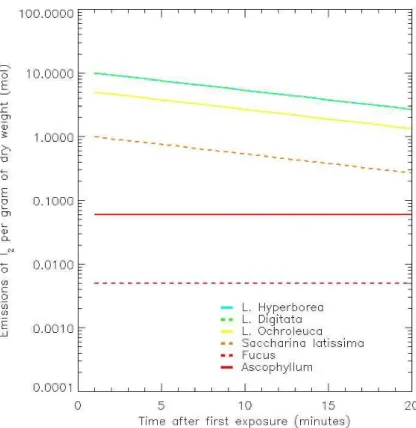
2.2 Emission rates from exposed macroalgae

Exposure rates for each species of macroalgae were converted into estimated emis-sion rates based on the time since first exposure of each grid square. Emisemis-sions in picomoles per minute per gramme fresh weight were taken from Ball et al. (2009) for all species exceptL. ochroleuca, for which measured data were not available, and an

20

assumed emission rate intermediate betweenL. digitataandSaccharina latissimawas used. All emission rates over time since first exposure are shown in Fig. 3. Emission rates for each species are assumed to be constant after 20 min of continuous exposure. These emission rates were converted into emissions per m2 using the assumptions shown in Table 1 of mass by species. Emissions each minute were assumed to mix

25

(7)

ACPD

9, 21165–21198, 2009

R. J. Leigh et al.

Title Page

Tables Figures

◭ ◮

Back Close

Full Screen / Esc

Interactive Discussion Actinic fluxes were measured using a Metcon spectral radiometer (Edwards and

Monks, 2003), and photolysis frequencies of a number of trace gases calcuated, in-cluding molecular iodine (jI2). The model temporal resolution was matched to the

meteorological dataset sampling of 1 min, with the model run in GMT. The model was run on data from 5 to 28 September 2006.

5

2.3 Footprint analysis

Concentration footprints (as opposed to the more often used flux footprints) were calcu-lated for a range of wind velocities and representative meteorological conditions (deter-mined from the measured data) using the analytical approximation of Schmid (1994). The model is a numerical solution to an analytical approximation of the

advection-10

diffusion equations. While the heterogeneity of the upwind surface makes it rather difficult to draw firm conclusions about the exact form of the concentration footprint, the model is capable of providing sufficiently detailed estimates for the purposes of this simple study. Table 2 shows the range of model input parameters used to provide estimates of the concentration footprint for the range of conditions encountered during

15

the field study period.

The surface roughness lengths used were 0.03 m where the fetch was across the inter-tidal zone. For the water surfaces encountered at high tide, z₀ was determined using the relationship described by Zilitinkevich (1969)

z₀₌c₁v u_∗+

u2_∗

c₂g (1)

20

whereu_∗ is the friction velocity, g the acceleration due to gravity, v is the kinematic viscosity, and c₁ and c₂ are coefficients with highly variable values estimated to be between (forc₁) 0.0–0.48, and (c₂) from∞to 81.1. In this study intermediate values of 0.1 and 32.0 were used.

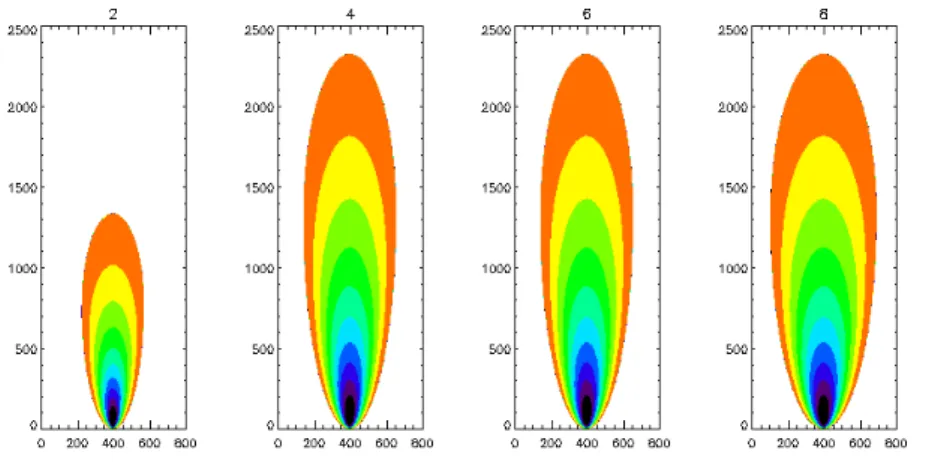
Using this technique, footprints were calculated at 2, 4, 6, 8, and 10 m/s windspeeds,

25

(8)

ACPD

9, 21165–21198, 2009

R. J. Leigh et al.

Title Page

Tables Figures

◭ ◮

Back Close

Full Screen / Esc

Interactive Discussion used in the model to characterise anticipated transport of emissions to the site and the

LP-DOAS line of sight. Linear interpolations between calculated footprints were used to smooth transitions from each calculated footprint scenario. Wind direction at the site was used to rotate the footprint accordingly. Following scaling and rotation, the footprint for each time step was applyed to the emissions grid to estimate the concentration

5

both at the site, and along the LP-DOAS line of sight. Footprints for the LP-DOAS were obtained through integration along the line of sight, examples of each footprint are shown in Figs. 8 and 9

3 Model results

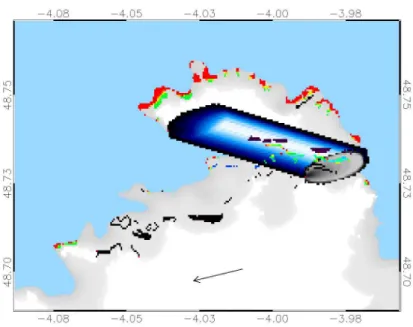
For each model timestep, the exposed regions of macroalgae were calculated, and

10

emissions estimated based on the length of exposure of each grid cell. The timeseries of temporal input parameters and calculated exposure for each species is shown in Fig. 5. Two example snap-shots of model steps are shown in Figs. 8 and 9. The “curtain” e_ffect during an ebb tide is shown in Fig. 8, as the initial exposure causes a burst of high I2emissions. Emissions are lower and more uniform during the flow tide, 15

reflected in the shape of total regional emission curves in Fig. 5.

4 BBCRDS measurements

A broadband cavity ringdown spectrometer was deployed from a shipping container sited on the jetty in front of the SBR, adjacent to the containers housing the cam-paign’s other in situ instruments. Broadband cavity ringdown spectroscopy (BBCRDS)

20

(9)

ACPD

9, 21165–21198, 2009

R. J. Leigh et al.

Title Page Abstract Introduction Conclusions References Tables Figures ◭ ◮ ◭ ◮ Back Close

Full Screen / Esc

Interactive Discussion 560–570 nm. Other atmospheric gases (H₂O, NO₂ and the oxygen dimer O₄) also

absorb at these wavelengths and thus contribute to the measured BBCRDS spectra. The present BBCRDS system is based on an instrument that previously measured I₂ at Mace Head (Ireland) during the 2002 NAMBLEX campaign (Saiz-Lopez et al., 2006) and that was described in detail by Bitter et al. (2005). In the intervening

5

years, the instrument’s performance has been enhanced significantly by upgrading several key components, notably a new laser system that yields pulsed broadband light with a factor of two wider bandwidth at green wavelengths, a new clocked CCD camera and improved analysis software/spectral fitting routines. Briefly: a broad-band dye laser pumped by a 532 nm Nd:YAG laser (Sirah Cobra and Surelight I-20;

10

20 Hz repetition rate) generated light pulses with an approximately Gaussian emission spectrum centered at 563 nm (FWHM=5.2 nm). This light was directed into a 187 cm long ringdown cavity formed by two highly reflective mirrors (Los Gatos, peak reflec-tivity₌99.993% at 570 nm). Light exiting the ringdown cavity was collected and con-veyed through a 100µm core diameter fibre optic cable to an imaging spectrograph

15

(Chromex 250is) where it was dispersed in wavelength and imaged onto a clocked CCD camera (XCam CCDRem2). The time evolution of individual ringdown events was recorded simultaneously at 512 different wavelengths, one for each pixel row of the detector, and light from 50 ringdown events was integrated on the CCD camera before storing the data to a computer. Wavelength resolved ringdown times were

pro-20

duced by fitting the ringdown decay in each pixel row (j₌1 to 512). The sampled absorption spectrum was then calculated from sets of ringdown times measured when the cavity contained the sample,τ(λ_j), and when flushed with dry nitrogen,τ₀(λ_j):

α(λ_j)=RL c

1

τ(λ_j)− 1

τ₀(λ_j)

!

=X

n

α_n(λ_j)+α_con(λ_j) (2)

wherec is the speed of light, R_L is the fraction of the cavity that is occupied by

ab-25

sorbing species, α_n(λ_j) is the wavelength dependent absorption coefficient of the nth molecular absorber andα_con(λ_j) is the absorption coe_fficient due to all other

(10)

ACPD

9, 21165–21198, 2009

R. J. Leigh et al.

Title Page

Tables Figures

◭ ◮

Back Close

Full Screen / Esc

Interactive Discussion tured contributions to the spectrum (mainly aerosol extinction). During the first part of

the campaign (before 16 September), the cavity was located inside the shipping con-tainer and ambient air was drawn into the cavity at 3 l per minute. The cavity was then moved onto the roof of the contrainer and operated in an open-path configuration for the remainder of the campaign. In both cases, appropriate corrections (Shillings, 2009)

5

were made to account for exclusion of the atmospheric sample from the cavitys mirror mounts which were purged with dry nitrogen to prevent contamination of the optical surfaces (i.e. theR_Lterm in Eq. 2).

BBCRDS absorption spectra were averaged to a time resolution of 5 min and the known absorptions due to ambient H2O (humidity meter) and O4(atmospheric oxygen 10

concentration) were subtracted. The concentrations of I₂and NO₂were then retrieved from a multivariate fit of reference absorption cross sections to the structured features remaining in the sample’s absorption spectrum using an analysis similar to that de-veloped for di_fferential optical absorption spectroscopy (DOAS) (Platt, 1999; Ball and Jones, 2003; Ball et al., 2009). NO2 cross sections were taken from Vandaele et al. 15

(1996) and were degraded to the 0.12 nm FWHM instrumental resolution. I2cross

sec-tions were derived from the PGOPHER spectral simulation program (Western, Access: September 2009; Martin et al., 1986) and were scaled to reproduce the differential cross sections reported by Saiz-Lopez et al. (2004). The top panel of Fig. 7 shows an example BBCRDS spectrum obtained during the campaign, after subtraction of the

20

known absorptions due to H2O and O4and a fitted quadratic function accounting for all

unstructured absorptionsα_con(λ_j). The central and lower panels show respectively the I₂ and NO₂ contributions to the measured absorption overlaid by their fitted reference spectra from the DOAS fitting routine. During the RHaMBLe campaign, the precision of the spectral retrievals was typically 10 pptv for I2and 0.2 ppbv for NO2(1σuncertainty, 25

304 s averaging time). Although not the principal target of this deployment, co-retrieval the NO2concentrations served as an important quality assurance parameter with which

to monitor the BBCRDS instrument’s performance. Throughout the campaign, the NO2

(11)

ACPD

9, 21165–21198, 2009

R. J. Leigh et al.

Title Page

Tables Figures

◭ ◮

Back Close

Full Screen / Esc

Interactive Discussion NO₂measurements made by the University of York’s NOxy chemiluminescence

instru-ment (McFiggans et al., 2009). For example, the gradient of a correlation plot of NO2

concentrations recorded by the two instruments on 14–15 September was 0.98±0.03.

5 Measurements taken by long path DOAS

During September 2006 the Long Path Differential Optical Absorption Spectroscopy

5

(LP-DOAS) technique (Plane and Saiz-Lopez, 2006) was used to measure the con-centrations of I₂, OIO, IO and NO₃. The absorption path extended 3.35 km from the SBR (48.728 latitude,−3.988 longitude), to a small outcrop of the Ile de Batz (48.74 lati-tude,−4.036 longitude), where a retroreflector array was placed to fold the optical path. The total optical path length was 6.7 km and the beam was 7 to 12 m above the mean

10

sea level. Details of the DOAS instrument employed can be found elsewhere (Ma-hajan et al., 2009; Saiz-Lopez and Plane, 2004). Briefly, spectra were recorded with 0.25 nm resolution before being converted into differential optical density spectra and the contributions of individual species determined by simultaneous fitting their absorp-tion cross-secabsorp-tions using singular value decomposiabsorp-tion (Plane and Saiz-Lopez, 2006).

15

Integrated I₂concentrations along the line of sight (Saiz-Lopez and Plane, 2004) were retrieved in the 535–575 nm window on a number of days and nights. Results from this instrument are presented comprehensively in Mahajan et al. (2009). Footprints for the LP-DOAS instrument were calculated using the same footprint model, assuming an 8 m path height, integrated and normalised along the line of sight. This provides a

20

modelled integrated measurement which sampled a significant proportion of the region (see Fig. 9. The relationship between regional emissions, maximum above-surface modelled concentrations, and the LP-DOAS measurements is shown in Fig. 6.

(12)

ACPD

9, 21165–21198, 2009

R. J. Leigh et al.

Title Page

Tables Figures

◭ ◮

Back Close

Full Screen / Esc

5.1 Calculation of total emissions and modelled exposure at the site and along the LP-DOAS line of sight

The total regional emissions were calculated within the model grid for each minute. Site and LP-DOAS footprints were calculated given wind speed, wind direction, and tidal height. The travel time within the footprint was estimated from windspeed, allowing

5

photolytic destruction to be calculated from the travel time of the molecular iodine to the site. Although no chemical modelling was attempted along the lines of Mahajan et al. (2009), a simple recycling parameter was also included in this work, permitting a proportion of photo-dissociated I₂to be instantly reformed. This recyling was achieved through modification of the photolytic destruction process from

10

I2(t)=I2(0)ejI2·t (3)

to

I₂₍_t₎=I₂₍₀₎ejI2·(1−R)·t ₍₄₎

Where: I2(t)is the volume mixing ratio of I2at time t, I2(0) is the volume mixing ratio of

I2at time 0 directly above the emission source. jI2is the photolysis frequency of I2as 15

measured by a spectral radiometer.Ris the assumed recycling rate set here toR=0.1, i.e. 10% of the I2that is photolysed is reformed by subsequent chemistry (c.f. Mahajan

et al., 2009).

Figure 6 shows total calculated regional emissions, the modelled I₂ mixing ratios in air advected to the measurement site (BBCRDS) and the mean I2 mixing ratio in 20

the air sampled along the LP-DOAS line of sight for three I2 loss scenarios: (I) no I2

(13)

ACPD

9, 21165–21198, 2009

R. J. Leigh et al.

Title Page

Tables Figures

◭ ◮

Back Close

Full Screen / Esc

6 Comparison of modelled and measured I₂

The full timeseries of modelled data for the BBCRDS and LP-DOAS instruments is shown in Fig. 6. The impact of photolytic destruction during the day is demonstrated by the almost complete removal of I2 predicted during daylight hours, despite significant

emission events.

5

There were unfortunately very few periods during which the LP-DOAS and BBCRDS systems were both operational on the same day. On 14 September, the LP-DOAS was operational in the morning, and the BBCRDS performed well overnight to the 15 September. Data from these instruments is plotted with model data in Fig. 10. The windspeed on 14 September rose from approximately 0 at midnight (14.0) to 1 ms−1 10

by 14.05 and 3 ms−1 by 14.1. The LP-DOAS measurements are in some cases up to four times the modelled concentration, although peak concentrations at the site are modelled to reach the 25 pptv level. The temporal structure of the measured I₂ does correlate with significant emissions and variable meteorological conditions. Similar structures are shown in Figs. 12 and 13 showing data from 5 and 19 September

re-15

spectively.

Model I2concentrations during the day are displayed with photolytic destruction and

recycling (at 10%) included (solid lines) and with all destruction processes switched off (dashed lines). The BBCRDS measurements during the morning of the 15 September, shown in Fig. 10 suggest agreement between the model and BBCRDS data, with

con-20

centrations at site being significantly more variable than along the averaged LP-DOAS line of sight. This is an expected consequence of the averaging over larger spatial scales of the LP-DOAS technique with respect to the point measurement modelled at site for the BBCRDS instrument. Concentrations at site were both measured and modelled over 40 pptv during nighttime periods. The primary contributions to these

25

concentrations are local emission sources, rather than the larger beds of L. digitata

andL. hyperborea, which remained beyond the site footprint and subject to complete photolytic destruction.

(14)

ACPD

9, 21165–21198, 2009

R. J. Leigh et al.

Title Page

Tables Figures

◭ ◮

Back Close

Full Screen / Esc

Interactive Discussion Measurements by the BBCRDS during hours of sunlight on 14 September (Fig. 10)

and 10 September (Fig. 11) show significant correlations and magnitude agreement with model predictions with all destruction processes switched off. This is suspected to be a result of local emission sources around the site, which are not included in the ex-isting maps used as model inputs. Such significant reductions in photolytic destruction

5

are not physically reasonable, but are a useful mechanism to explore a combination of alternative explanations including enhanced local emissions, chemical recycling, or a significant alternative source of molecular iodine through recyling or processing of other macroalgal emissions.

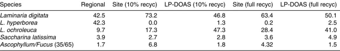
Total regional emissions were classified during this measurement period by species,

10

in addition to exposures of LP-DOAS and BBCRDS instruments, providing informa-tion on the main contributing species to each measurement technique. Proporinforma-tions of emissions from each species measured at site, and with the LP-DOAS technique are shown in Table 3. Given that the LP-DOAS line of sight fell directly over a bed of

L. ochroleuca, the significant contribution of this species to LP-DOAS measurements

15

is expected. Emissions fromL. ochroleucaare relatively poorly constrained relative to someL.species. One potential source of the additional I₂in the LP-DOAS measure-ments is therefore provided by an increased emission rate fromL. ochroleuca, which would impact the LP-DOAS measurements more than the site.

Despite the relative scarcity of L. digitataaround the measurement site, and under

20

the LP-DOAS line of sight, contributions from this species are significant, whileL. hy-perborea provided over 40% of the total regional emissions and yet consituted less than 0.5% and 2.5% of BBCRDS and LP-DOAS measurements respectively.

7 Conclusions

A simple dynamical model was produced to examine the potential sensitivity of in situ

25

(15)

ACPD

9, 21165–21198, 2009

R. J. Leigh et al.

Title Page

Tables Figures

◭ ◮

Back Close

Full Screen / Esc

Interactive Discussion emissions by species, concentrations aboveL. hyperborea and L. digitatabeds were

predicted at 2.5 ppbv. Total regional emissions for the 100 km2zone have been mod-elled to be up to 1.5× 019 molecules per second during the lowest tides. Modelled concentrations for the LP-DOAS instrument reach a maximum of 30 pptv, and have a similar structure, although lower concentrations compared with measurements. With

5

the significant contribution of L. ochroleuca to this measurement, an increase in the stated emission rate from this species provides one potential explanation.

Modelled concentrations at the site are significantly more variable, but can reach up to 80 pptv during major nighttime episodes. Agreement has been demonstrated be-tween the BBCRDS measurements and modelled concentrations around the 20 pptv

10

level. During the day, photolytic destruction should destroy the significant majority of primarily produced I2 prior to measurement by either technique. There are

how-ever significant measured concentrations from the BBCRDS, correlating with modelled structures of I₂ when destruction processes are eliminated, which merit further inves-tigation. Such features may be a result of unmodelled local emissions, a significant

15

missing recycling or source component, or correlated errors in both model and mea-surement.

Such temporal and spatial analysis is recommended for future measurements in such spatially inhomogeneous and temporal variable emission fields, ideally coupled with a suitable chemistry scheme. When considering concurrent, or almost concurrent

20

measurements of I₂, IO, and particle formation, the rapidly varying meteorology cou-pled with varying emissions and differing process timescales render more simplistic analyses problematic. Considerations of the rapid destruction processes for I2, known

chemical recycling paths for IO, and the time dependence of observable particle for-mation in coastal regions is discussed in more detail in McFiggans et al. (2009) and

25

references therein.

(16)

ACPD

9, 21165–21198, 2009

R. J. Leigh et al.

Title Page

Tables Figures

◭ ◮

Back Close

Full Screen / Esc

Interactive Discussion Acknowledgements. The authors would like to thank the staff at the Station Biologique de

Roscoff for their significant assistance during the RHaMBLE project, and the Natural Envi-ronment Research Council for funding the RHaMBLE campaign. Deployment of the BBCRDS instrument to the RHaMBLE campaign was made possible through a grant from the Natural Environment Research Council NE/D00652X/1.

5

References

Arzel, P.: Les laminaires sur les c ôtes bretonnes, évolution de l’exploitation et de la flottille de p êche, état actuel et perspectives., Edition de l’Ifremer, p. 139, 1998. 21170

Bajjouk, T., Guillaumont, B., and Populus, J.: Application of Airborne Imaging Spectrometry System Data to Intertidal Seaweed Classification and Mapping, Hydrobiologia, 327, 463–

10

471, 1996. 21169

Ball, S., Hollingsworth, A. M., Humbles, J., Leblanc, C., Potin, P., Langridge, J. M., Lecrane, J.-P., and McFiggans, G.: Spectroscopic Studies of Molecular Iodine Emitted into the Gas Phase by Seaweed., Atmospheric Chemistry and Physics, this issue, XX, 2009. 21170, 21174, 21188

15

Ball, S. M. and Jones, R.: Broad-band cavity ring-down spectroscopy, Chem Rev., 103, 5239– 5262, 2003. 21174

Ball, S. M. and Jones, R.: Broadband Cavity Ring-Down Spectroscopy, in Cavity Ring-Down Spectroscopy: Techniques and Applications, Blackwell Publishing, 2009. 21172

Bitter, M., Ball, S., Povey, I., and Jones, R.: A Broadband Cavity Ringdown Spectrometer for

20

In-Situ Measurements of Atmospheric Trace Gases, Atmos. Chem. Phys., 5, 3491–3532, 2005, http://www.atmos-chem-phys.net/5/3491/2005/. 21172, 21173

Braud, J.-P.: Etude de quelques param ètres écologiques, biologiques et biochimiques chez une ph éophyc ée des c ôtes bretonnes Laminaria ochroleuca, Revue des Travaux de l’Institut des P êches Maritimes (ISTPM), 38, 1974. 21169

25

Edwards, G. D. and Monks, P.: Performance of a single monochromator diode array spectro-radiometer for the determination of actinic flux and atmospheric photolysis frequencies, J. Geophys. Res., 108, 8546, doi:10.1029/2002JD002844, 2003. 21171

(17)

ACPD

9, 21165–21198, 2009

R. J. Leigh et al.

Title Page Abstract Introduction Conclusions References Tables Figures ◭ ◮ ◭ ◮ Back Close

Full Screen / Esc

Interactive Discussion Goll ´ety, C., Mign ´e, A., and D., D.: Benthic metabolism on a sheltered rocky shore: role of the

canopy in the carbon budget, J. Phycol., 44, 1146–1153, 2008. 21170

L ¨uning, K.: Seaweeds: Their environment, biogeography, and ecophysiology, Wiley, 527 pp., 1990. 21169, 21170

5

Mahajan, A., Oetjen, H., Saiz-Lopez, A., Lee, J. D., McFiggans, G. B., and Plane, J. M. C.: Re-active iodine species in a semi-polluted environment, Geophys. Res. Lett., 2009GL038018, accepted, 2009. 21175, 21176

Martin, F., Bacis, R., Churassy, S., and Verg `es, J.: Laser-induced-fluorescence Fourier trans-form spectrometry of the X₁Σ+g state of I2: Extensive analysis of the B

3

Π+u →X

1

Σ+g fluores-10

cence spectrum of127I2, J. Molec. Spectrosc., 116, 71, 1986. 21174

McFiggans, G., Bale, C. S. E., Ball, S., Beaumes, J. M., Bloss, W. J., Carpenter, L. J., Dorsey, J., Dunk, R., Flynn, M. J., Furneaux, K. L., Gallagher, M. W., Heard, D. E., Hollingsworth, A. M., Hornsby, K. E., Ingham, T., Jones, C. E., Jones, R. L., Kramer, L. K., Langridge, J. M., Leblanc, C., LeCrane, J.-P., Lee, J. D., Leigh, R. J., Longley, I., Mahajan, A. S., Monks, P. S.,

15

Oetjen, H., Orr-Ewing, A. J., Plane, J. M. C., Potin, P., Shillings, A. J. L., Thomas, F., von Glasow, R., Wada, R., Whalley, L. K., and Whitehead, J. D.: Iodine-mediated coastal particle formation: an overview of the Reative Halogens in the Marine Boundary Layer (RHaMBLe) Roscoffcoastal studey, Atmos. Chem. Phys. Discuss., to be submitted, 2009. 21168, 21175, 21179

20

Plane, J. M. C. and Saiz-Lopez, A.: Analytical Techniques for Atmospheric Measurement, Blackwell, 510 pp., 2006. 21175

Platt, U.: Modern methods for the measurement of atmospheric trace gases, Phys. Chem. Chem. Phys., 1, 5409–5415, 1999. 21174

Saiz-Lopez, A. and Plane, J. M. C.: Novel iodine chemistry in the marine boundary layer,

25

Geophys. Res. Lett., 31, L04112, doi:10.1029/2003GL019215, 2004. 21175

Saiz-Lopez, A., Saunders, R., Joseph, D. M., Ashworth, S. H., and Plane, J. M. C.: Absolute absorption cross-section and photolysis rate of I2, Atmos. Chem. Phys., 4, 1443–1450, 2004, http://www.atmos-chem-phys.net/4/1443/2004/. 21174

Saiz-Lopez, A., Plane, J. M. C., McFiggans, G., Williams, P. I., Ball, S. M., Bitter, M., Jones,

30

R. L., Hongwei, C., and Hoffmann, T.: Modelling molecular iodine emissions in a coastal marine environment: the link to new particle formation, Atmos. Chem. Phys., 6, 883–895, 2006, http://www.atmos-chem-phys.net/6/883/2006/. 21173

Schmid, H. P.: Source areas for scalars and scalar fluxes, Bound. Lay. Meteorol., 67, 293–318,

(18)

ACPD

9, 21165–21198, 2009

R. J. Leigh et al.

Title Page

Tables Figures

◭ ◮

Back Close

Full Screen / Esc

Interactive Discussion 1994. 21171

Shillings, A.: Atmospheric Applications of Broadband Cavity Ringdown Spectroscopy, PhD. Thesis, University of Cambridge, 2009. 21174

Vandaele, A., Hermans, C., Simon, P., Van Roozendael, M., Guilmot, J., Carleer, M., and Colin,

5

R.: Fourier Transform Measurement of NO₂Absorption Cross-sections in the Visible Range at Room Temperature, J. Atmos. Chem., 25, 289–305, 1996. 21174

Western, C.: PGOPHER: a Program for Simulating Rotational Structure, Available: University of Bristol, http://pgopher.chm.bris.ac.uk, last access: September 2009. 21174

(19)

ACPD

9, 21165–21198, 2009

R. J. Leigh et al.

Title Page

Tables Figures

◭ ◮

Back Close

Full Screen / Esc

Table 1.Assumptions used to convert mass per gramme into mass per m2.

Species Minimum Maximum Average Average Average

Depth depth biomass volumic mass volume

(m) (m) (kg FW/m2) (kg FW/m2) (m3/m2)

L. digitata +0.5 −1.0 10 320 0.03

L. ochroleuca 0 −5.0 10 315 0.03

L. hyperborea 0 20.0 10 310 0.03

Saccharina latissima +0.5 −2.0 10 140 0.07

Ascophyllum/Fucus(35/65) +1.5 +6.0 8 230 0.035

(20)

ACPD

9, 21165–21198, 2009

R. J. Leigh et al.

Title Page

Tables Figures

◭ ◮

Back Close

Full Screen / Esc

Table 2. Parameters used as input into the footprint model. Note that while the roughness length varies over water, a constant value of 0.03 m was used for runs at low tide across the inter-tidal zone. All 10 sets of parameters were run for both high and low tide cases. Measurement height was 8 m.Symbols are: z₀ – surface roughness length, σ_v – transverse velocity variance,u_∗ – friction velocity, L – Obukhov length.

Day Night

U (ms-1) z₀(m) σv(ms-1) u∗(ms-1) L(m) z0(m) σv(ms-1) u∗(ms-1) L(m)

2.00 0.00100 0.40 0.20 −25 0.00100 0.40 0.15 100

4.00 0.00100 0.80 0.40 −100 0.00100 0.60 0.30 200

6.00 0.00115 1.20 0.60 −100 0.00100 0.9 0.45 300

8.00 0.00156 1.60 0.70 −100 0.00115 1.10 0.60 200

(21)

ACPD

9, 21165–21198, 2009

R. J. Leigh et al.

Title Page

Tables Figures

◭ ◮

Back Close

Full Screen / Esc

Table 3.Percentage of total regional emissions visible at site.

Species Regional Site (10% recyc) LP-DOAS (10% recyc) Site (full recyc) LP-DOAS (full recyc)

Laminaria digitata 42.5 73.2 46.8 63.4 50.1

L. hyperborea 42.3 0.0 1.3 0.2 2.5

L. ochroleuca 9.7 17.3 47.3 28.4 41.0

Saccharina latissima 3.9 2.7 2.8 3.6 4.9

Ascophyllum/Fucus(35/65) 1.7 6.8 1.8 4.32 1.5

(22)

ACPD

9, 21165–21198, 2009

R. J. Leigh et al.

Title Page

Tables Figures

◭ ◮

Back Close

Full Screen / Esc

(23)

ACPD

9, 21165–21198, 2009

R. J. Leigh et al.

Title Page

Tables Figures

◭ ◮

Back Close

Full Screen / Esc

Fig. 2.The kelp bed at the Rocher du Loup, at a low tide of about 0.5 m dominated byL. digitata (kelp) and just above a belt ofHimanthalia elongata(fucoid).

(24)

ACPD

9, 21165–21198, 2009

R. J. Leigh et al.

Title Page

Tables Figures

◭ ◮

Back Close

Full Screen / Esc

(25)

ACPD

9, 21165–21198, 2009

R. J. Leigh et al.

Title Page

Tables Figures

◭ ◮

Back Close

Full Screen / Esc

Fig. 4.Footprints used in this model, at 2, 4, 6, 8 and 10 m/s windspeed.

(26)

ACPD

9, 21165–21198, 2009

R. J. Leigh et al.

Title Page

Tables Figures

◭ ◮

Back Close

Full Screen / Esc

(27)

ACPD

9, 21165–21198, 2009

R. J. Leigh et al.

Title Page

Tables Figures

◭ ◮

Back Close

Full Screen / Esc

Fig. 6. Output from the model. From Top down, Regional emissions as calculated by the model, maximum calcu-lated concentrations above macroalgal beds, site exposure based on footprint analysis calcucalcu-lated for no destruction processes, with photodissociation, and with photodissociation coupled with 10% recycling back into I₂.

(28)

ACPD

9, 21165–21198, 2009

R. J. Leigh et al.

Title Page

Tables Figures

◭ ◮

Back Close

Full Screen / Esc

(29)

ACPD

9, 21165–21198, 2009

R. J. Leigh et al.

Title Page

Tables Figures

◭ ◮

Back Close

Full Screen / Esc

Fig. 8. Model timestep from 10:32 p.m. on 7 September 2006 during an ebb tide, one of the highest concentrations predicted at site. The windspeed and direction at this time was 5.65 m/s and 79.7 degrees respectively, with the tide 0.85 m below the datum). LP-DOAS and site footprints are shown, overlayed by estimated emissions, with red denoting an emission rate of 1_×1017molecules per grid square per second.

(30)

ACPD

9, 21165–21198, 2009

R. J. Leigh et al.

Title Page

Tables Figures

◭ ◮

Back Close

Full Screen / Esc

(31)

ACPD

9, 21165–21198, 2009

R. J. Leigh et al.

Title Page

Tables Figures

◭ ◮

Back Close

Full Screen / Esc

Fig. 10. Modelled and measured data from 14 September 2006. Shown are; jI₂ (red), tide height (black), modelled concentration at site and along the LP-DOAS line of site with photolytic destruction and 10% recycling (solid green and blue lines respectively), modelled concentra-tion at site and along the LP-DOAS line of site with no destrucconcentra-tion processes modelled (dashed green and blue lines respectively), and measurements from the LP-DOAS and BBCRDS instru-ments(blue and green dots respectively, with error bars).

(32)

ACPD

9, 21165–21198, 2009

R. J. Leigh et al.

Title Page

Tables Figures

◭ ◮

Back Close

Full Screen / Esc

(33)

ACPD

9, 21165–21198, 2009

R. J. Leigh et al.

Title Page

Tables Figures

◭ ◮

Back Close

Full Screen / Esc

Fig. 12.Modelled and measured data from 5 September 2006. Shown are;jI₂(red), tide height (black), modelled concentration at site and along the LP-DOAS line of site with photolytic de-struction and 10% recycling (solid green and blue lines respectively), modelled concentration at site and along the LP-DOAS line of site with no destruction processes modelled (dashed green and blue lines respectively), and measurements from the LP-DOAS and BBCRDS in-struments(blue and green dots respectively, with error bars).

(34)

ACPD

9, 21165–21198, 2009

R. J. Leigh et al.

Title Page

Tables Figures

◭ ◮

Back Close

Full Screen / Esc