A sea surface reflectance model for (A)ATSR, and application to aerosol retrievals

(1)

AMTD

3, 1023–1098, 2010

A sea surface reflectance model for

(A)ATSR

A. M. Sayer et al.

Title Page Abstract Introduction Conclusions References Tables Figures

◭ ◮

Back Close Full Screen / Esc

Printer-friendly Version Interactive Discussion Atmos. Meas. Tech. Discuss., 3, 1023–1098, 2010

www.atmos-meas-tech-discuss.net/3/1023/2010/ © Author(s) 2010. This work is distributed under the Creative Commons Attribution 3.0 License.

Atmospheric Measurement Techniques Discussions

This discussion paper is/has been under review for the journal Atmospheric Measure-ment Techniques (AMT). Please refer to the corresponding final paper in AMT

if available.

A sea surface reflectance model for

(A)ATSR, and application to aerosol

retrievals

A. M. Sayer, G. E. Thomas, and R. G. Grainger

Atmospheric, Oceanic & Planetary Physics, Clarendon Laboratory, Parks Road, Oxford, OX1 3PU, UK

Received: 5 March 2010 – Accepted: 13 March 2010 – Published: 18 March 2010 Correspondence to: A. M. Sayer (sayer@atm.ox.ac.uk)

(2)

AMTD

3, 1023–1098, 2010

(A)ATSR

A. M. Sayer et al.

◭ ◮

Printer-friendly Version Interactive Discussion

Abstract

A model of the sea surface bidirectional reflectance distribution function (BRDF) is pre-sented for the visible and near-IR channels (over the spectral range 550 nm to 1.6 µm) of the dual-viewing Along-Track Scanning Radiometers (ATSRs). The intended appli-cation is as part of the Oxford-RAL Aerosols and Clouds (ORAC) retrieval scheme. 5

The model accounts for contributions to the observed reflectance from whitecaps, sun-glint and underlight. Uncertainties in the parametrisations used in the BRDF model are propagated through into the forward model and retrieved state. The new BRDF model off_{ers improved coverage over previous methods, as retrievals are possible into} the sun-glint region, through the ATSR dual-viewing system. The new model has been 10

applied in the ORAC aerosol retrieval algorithm to process Advanced ATSR (AATSR) data from September 2004 over the south-eastern Pacific. The assumed error bud-get is shown to be generally appropriate, meaning the retrieved states are consistent with the measurements and a priori assumptions. The resulting field of aerosol op-tical depth (AOD) is compared with colocated MODIS-Terra observations, AERONET 15

observations at Tahiti, and cruises over the oceanic region. MODIS and AATSR show similar spatial distributions of AOD, although MODIS reports values which are larger and more variable. It is suggested that assumptions in the MODIS aerosol retrieval al-gorithm may lead to a positive bias in MODIS AOD of order 0.01 at 550 nm over ocean regions where the wind speed is high.

20

1 Introduction

The Intergovernmental Panel for Climate Change (IPCC) has identified aerosols as among the most uncertain contributions to radiative forcing (Penner et al., 2001, Forster et al., 2007). As approximately 70% of the Earth’s surface is covered by water, the ac-curate determination of aerosol loadings over ocean is critical to assess direct and indi-25

(3)

sur-AMTD

3, 1023–1098, 2010

(A)ATSR

A. M. Sayer et al.

◭ ◮

Printer-friendly Version Interactive Discussion face is dark, particularly compared to typical land surfaces, meaning the proportional

atmospheric contribution to the signal measured by imaging radiometers at the top-of-atmosphere (TOA) is higher for the same aerosol loading. However, typical oceanic aerosol loadings are low (see, for example, Smirnov et al., 2009), meaning the surface contribution is non-negligible. An exception to the rule of the ocean being dark is found 5

in sun-glint, whereby solar and satellite geometries lead to regions where the surface is very bright, typically in the tropics for near-nadir-viewing instruments. Parametrisa-tions of sun-glint are largely based on the approach of Cox and Munk (1954a), and most aerosol retrieval algorithms use a glint formulation to identify and mask out glint-aff_{ected regions before processing. This has the e}ff_{ect of reducing the spatial coverage} 10

of the derived aerosol dataset, particularly in the tropics.

A notable exception to this is given by O’Brien and Mitchell (1988), who relied on the predictable spatial variation of surface reflectance within large cloud-free portions of the sun-glint region to peform aerosol and wind speed retrievals from Advanced Very High Resolution Radiometer (AVHRR) data. This methodology has, however, seen 15

little application since.

Multiangle imaging instruments such as the Along-Track Scanning Radiometers (AT-SRs), Multiangle Imaging SpectroRadiometer (MISR) and POLarization and Direction-ality of the Earth’s Reflectances (POLDER) allow for an improved representation of surface anisotropy in aerosol retrieval algorithms, although over oceans measurements 20

from a single viewing geometry have been considered suffi_{cient to derive useful aerosol} information. The treatment of surface reflectance in some of these (single-view or mul-tiview) algorithms is described below. Typically, the primary quantity retrieved is the aerosol optical depth (AOD) at a mid-visible wavelength; many algorithms use a fixed surface reflectance, and some a fixed aerosol type. Regional diff_{erences exist in ocean} 25

(4)

Net-AMTD

3, 1023–1098, 2010

(A)ATSR

A. M. Sayer et al.

◭ ◮

Printer-friendly Version Interactive Discussion work (MAN, Smirnov et al., 2009) of ship-borne open ocean measurements is spatially

and temporally sparser. It is likely that some of the diff_{erences between these satellite} climatologies arise from the assumptions made about the ocean surface reflectance. Partially as a result of the comparative darkness of the ocean as compared to land surface reflectances, the various algorithms as summarised below tend to show little 5

change since their early versions.

The over-ocean aerosol retrieval algorithm for the MODerate resolution Imaging Spectroradiometer (MODIS) is described first by Tanr ´e et al. (1997), and the same basic algorithm is applied in the current Collection 5 of the dataset (Remer et al., 2005). The methodology is adapted from Koepke (1984), who defined glint, whitecap 10

(foam) and underlight (scattering from dissolved pigments) contributions to the surface reflectance. The glint formulation of Cox and Munk (1954a) is used with a fixed wind speed, whitecap and underlight contribution, and a glint threshold is defined in which no retrievals are performed (unless heavy dust loading is detected, in which case the re-trieval is attempted). The overall surface reflectance is fixed in the algorithm. Sediment 15

masks are used to remove pixels of high sediment loading, which are not accounted for by the reflectance algorithm. The MISR ocean aerosol retrieval algorithm (Martonchik et al., 1998) also uses the method of Koepke (1984).

Veefkind and de Leeuw (1998) use a similar algorithm and fixed surface reflectance to retrieve AOD over ocean as a mixture of two aerosol types (anthropogenic and 20

maritime) from ATSR-2 data. The nadir and forward views are used independently, and a comparison between the two views can be used as a consistency check. The study noted that errors in the TOA reflectance arising from an incorrect wind speed could lead to errors of 0.04–0.16 in nadir-view-derived AOD. As typical open ocean optical depths may be of this order (Smirnov et al., 2009), this is a significant possible 25

(5)

AMTD

3, 1023–1098, 2010

(A)ATSR

A. M. Sayer et al.

◭ ◮

Printer-friendly Version Interactive Discussion (2009c). This took a similar approach for sea surface reflectance although allowed the

absolute magnitude to vary (while fixing the spectral shape of the surface).

Two-channel aerosol retrieval algorithms are presented for AVHRR by Higurashi and Nakajima (1999) and Mischenko et al. (1999): these use fixed glint-based surface reflectances calculated as described in Nakajima and Tanaka (1983) and Mischenko 5

and Travis (1997) respectively. They also consider the impacts of the simple reflectance model on the retrieved AOD and ˚Angstrom exponent, noting that it can be significant for cases of high wind or pigment concentrations, or low aerosol loadings.

Dedicated ocean colour sensors such as the Sea-viewing Wide Field-of-view Sen-sor (SeaWiFS) focus on the retrieval of parameters such as chlorophyll-aconcentration 10

and treat aerosol as part of an atmospheric correction term. Approximations made in surface reflectance models, such as the “black pixel approximation” (that the water-leaving radiance in the nIR is negligible), have been shown to negatively impact upon the quality of retrieved ocean colour parameters (Siegel et al., 2000). Sano (2004) describes an algorithm for retrieval of AOD, ˚Angstrom exponent and aerosol refrac-15

tive index from POLDER reflectance and polarisation measurements at 670 nm and 865 nm, making use of the black pixel approximation along with the glint formulation of Cox and Munk (1954a).

This work describes a new algorithm for the calculation of sea surface reflectance, drawing upon the methodology of Koepke (1984). The intended application is as part 20

of the Oxford-RAL Aerosol and Clouds (ORAC) scheme. This is discussed here in the context of aerosol retrievals, although the model may also be applied in the case of optically-thin cloud (where the surface contribution at TOA is non-negligible). As each sensor is diff_{erent, previous assumptions must be reevaluated, and more recent work} taken into account, to create a model suitable for the ATSRs. By modelling accurately 25

(6)

AMTD

3, 1023–1098, 2010

(A)ATSR

A. M. Sayer et al.

◭ ◮

Printer-friendly Version Interactive Discussion channels on the ATSRs may be used. Furthermore, in ORAC, unlike many

previously-described algorithms, the surface reflectance is not fixed, adding some flexibility in those cases in which the assumed surface reflectance is incorrect.

2 Overview of the ORAC-(A)ATSR aerosol retrieval

2.1 The (A)ATSR instruments

5

The ATSR series consists of three instruments: ATSR-1 (aboard ERS-1), launched in 1991, ATSR-2 (aboard ERS-2), launched in 1995, and the Advanced ATSR (AATSR, aboard Envisat), launched in 2002. The ATSRs were primarily designed for measure-ment of sea surface temperature (Z ´avody et al., 1995). While ATSR-1 measured ra-diance at one wavelength in the near-infrared and three in the thermal infrared part 10

of the spectrum, ATSR-2 and AATSR have an additional three channels in the visible region. It is these visible channels which are key to the instruments’ ability to provide data suitable for aerosol retrievals, and so ATSR-2 and AATSR, referred to from here as (A)ATSR, are considered here.

ERS-2 and Envisat are in Sun-synchronous polar orbit with a mean local solar equa-15

torial crossing time of 10:30 a.m. (ERS-2) or 10:00 a.m. (Envisat) for the descending node. The ATSR instruments are unique in that they use two views (near-simultaneous in time) with diff_{ering path lengths to discriminate between radiance from the surface} and radiance from the atmosphere. (A)ATSR measures at seven channels in the vis-ible and infrared; at present the first four (centred near 550 nm, 660 nm, 870 nm and 20

1.6 µm, known as channels 1–4 respectively) are used in the aerosol retrieval scheme. The additional bands are centred near 3.7 µm, 11 µm and 12 µm.

(7)

AMTD

3, 1023–1098, 2010

(A)ATSR

A. M. Sayer et al.

◭ ◮

R_TOA(θ_s,φ_s;θ_v,φ_v), which is defined

R_TOA(θ_s,φ_s;θ_v,φ_v)= Rλ2

λ₁πL r

λ̺(λ)d λ Rλ2

λ1cosθsE

i

λ̺(λ)d λ

(1)

whereθs,φs denote the illumination (solar) zenith and azimuth angles and θv,φv the

corresponding angles of view (the sensor) respectively. A channel is defined between wavelengthsλ₁,λ₂to have response̺(λ) . Finally Lr_λ is the radiance measured by the 5

instrument andE_λi is the TOA downward solar irradiance.

The area sampled by (A)ATSR consists of two curved swathes: a nadir view, looking down at zenith angles from 0◦–22◦, and a forward view inclined between 53◦–55◦to the normal to the surface. There are 555 pixels across the nadir swath (with a size of about 1 km2at the centre) and 371 across the forward swath (with a size of about 1.5 km2at 10

the centre). During each scan cycle the satellite moves approximately 1 km onward with respect to the Earth’s surface; after around 150 s the satellite has moved such that nadir view samples the same region, giving two views of the scene with diff_{ering path} lengths. Global coverage is achieved every 3–6 days depending on location. ATSR-2 operates in a narrow-swath mode over much of the ocean, reducing coverage by 15

approximately half, due to data-downlinking restrictions from the ERS-2 platform. (A)ATSR has an on-board visible calibration system consisting of an opal diff_user which views the Sun once per orbit. This, together with vicarious calibration against stable bright ground targets, means that the visible channel reflectances are known to an accuracy of 2–3% (Smith et al., 2002, 2008).

20

2.2 The ORAC retrieval

(8)

AMTD

3, 1023–1098, 2010

(A)ATSR

A. M. Sayer et al.

◭ ◮

Printer-friendly Version Interactive Discussion forward views of the first four channels. The retrieved state parameters (the “state

vec-tor”) are the aerosol optical depth at 550 nm (τ₅₅₀), the aerosol eff_{ective radius (}_r

e) and

the surface bihemispherical reflectance at each of the four channels used (R_dd_,₁,R_dd_,₂,

R_dd_,₃ andR_dd_,₄). The AOD is reported at 550 nm as this is the commonly-used stan-dard; the derived AOD may, however, be referenced to any wavelength, and is obtained 5

from all measurements simultaneously.

For computational speed, cloud-free forward and nadir-view data are typically aver-aged to a 10 km sinusoidal grid before the ORAC retrieval is performed. This averag-ing to a coarser resolution is known as “superpixellaverag-ing”. From here, the term “ground scene” is taken to refer to the data, superpixelled or not, used for an individual retrieval. 10

However, ORAC can in principle be performed at any resolution. The robust statistical basis of OE provides the following advantages:

1. Estimates of the quality of the retrieval solution (the retrieval “cost”) for each ground scene. This is essentially an error-weightedχ2test of the fit to the mea-surements at the retrieval solution, which provides a level of confidence as to the 15

results of any one retrieval.

2. Estimates of the random error on each retrieved parameter for each ground scene. These arise through knowledge of the uncertainty on the measurements and any a priori data, propagated through the forward model.

3. The ability (but not requirement) to use any a priori data available on the state 20

parameters. The model described in this work provides an a priori for the surface bihemispherical reflectance.

The retrieval forward model, presented in Thomas et al. (2009a), calculates the TOA reflectance for a given viewing geometry and state vector. It makes use of precal-culated lookup tables (LUTs) of atmospheric transmission and reflectance using the 25

(9)

AMTD

3, 1023–1098, 2010

(A)ATSR

A. M. Sayer et al.

◭ ◮

Printer-friendly Version Interactive Discussion (1998), and additionally a model for biomass burning aerosol drawn from Dubovik et al.

(2002). These models consist of mixtures of aerosol components, and diff_{erent e}ff ec-tive radii are obtained by altering their mixing ratios during the retrieval. Generally, the retrieval is attempted for each aerosol type. The most likely aerosol type may be cho-sen either by considering the model which resulted in the best fit to the measurements 5

(the lowest retrieval cost), or using other available information external to the retrieval.

2.3 Surface reflectance in the ORAC forward model

Schaepman-Strub et al. (2006) noted that in remote sensing terms relating to re-flectance were often misunderstood or applied ambiguously or incorrectly. They de-fined nomenclature for nine types of reflectance, using the framework of Nicodemus 10

et al. (1977), corresponding to the incoming and outgoing radiation that is either direc-tional, conical or hemispherical. The relevant geometric notation used throughout this work is given in Table 1. For clarity and conciseness of notation, spectral variability of the reflectances is implicit in the definitions and so omitted in the notation.

The most fundamental quantity is the bidirectional reflectance distribution function 15

(BRDF), denoted in the ORAC retrieval byR_bb:

R_bb(θ_s,φ_s;θ_v,φ_v)=∂L

r

λ(θs,φs;θv,φv)

∂E_λi(θ_s,φ_s) (2)

This defines the BRDF in terms of the proportionL_r of the incident irradianceE_i re-flected from direction (θ_s,φ_s) into direction (θ_v,φ_v). In this case, the point of incidence is the Sun and point of reflection is the satellite sensor. It has units of sr−1, and as a 20

ratio of infinitesimal quantities it (and other directional reflectances) may not be directly observed. In general use the term is defined as a surface property, although a TOA BRDF could also be defined as a conceptual analogue toRTOA. The BRDF is integrable

(10)

AMTD

3, 1023–1098, 2010

(A)ATSR

A. M. Sayer et al.

◭ ◮

Printer-friendly Version Interactive Discussion the radiant flux reflected under the same geometric conditions by an ideal Lambertian

surface, such that the bidirectional reflectance factor (BRF) is the BRDF multiplied by

π(Schaepman-Strub et al., 2006).

The closest observable equivalent to the BRF is the biconical (or conical-conical) reflectance factor (BCRF or CCRF), obtained by integrating the BRF over solid angles 5

ωto generate cones of incident and reflected light. Conical quantities become a good approximation for the related directional qualities when the solid angles of the cones are small. In this case the solid angle subtended by the Sun is small, as is the instrument’s instantaneous field of view (IFOV) of 1/777 rad.

For ambient lighting conditions there will be atmospheric contributions from diff usely-10

scattered light and absorption. These eff_{ects lead to the need for an “atmospheric} cor-rection” for ground-based sensing applications, or conversely they provide the “signal” for atmospheric sounding; i.e. the biconical reflectance observed at the TOA may have significantly diff_{erent spectral and angular characteristics to the biconical reflectance} just above the surface. Through optimal estimation, ORAC extracts the information 15

about both from the TOA measurements.

To account for the mixture of direct and diff_{use illumination the ORAC retrieval} for-ward model (Thomas et al., 2009a) treats the direct and diff_{use contributions to TOA} reflectance with separate terms, subjecting them to diff_{erent reflectances at ground,} and diff_{erent atmospheric transmittances. The surface reflectances required for direct} 20

and diff_{use radiance may be derived from the BRDF. Hence it becomes necessary to} define three types of surface reflectance in the forward model:

1. The surface BRDF,Rbb. This describes the reflection of the direct solar beam into

the viewing angle, and is a function of both solar and viewing angles. The BRDF is diff_{erent for each of AATSR’s viewing geometries. This is assumed equivalent} 25

to the CCRDF and so no integration over solid angle is performed.

(11)

AMTD

3, 1023–1098, 2010

(A)ATSR

A. M. Sayer et al.

◭ ◮

Printer-friendly Version Interactive Discussion reflection of incoming diff_{use radiance), and is a function of the solar angle. The}

short time delay between the forward and nadir views means that the solar angle and hence DHR are eff_{ectively identical for both views. This is sometimes referred} to as black-sky albedo, as incoming illumination comes from a sole direction.

3. The bihemispherical reflectance (BHR),R_dd. This describes the reflection of dif-5

fuse downwelling radiation, assumed isotropic. Hence it is independent of the geometry, and is the quantity retrieved by the retrieval algorithm. This is some-times referred to as white-sky albedo, as illumination arises from the whole of the sky.

In this notation the subscript b indicates a direct beam reflectance and d a diff_use 10

reflectance; the DHR Rbd, for example, denotes an incoming direct beam being

dif-fusely reflected. Given an analytical description of R_bb, the DHR for a given solar zenith angle may be obtained by integration over all satellite viewing zenith and relative (solar-satellite) azimuth angles:

R_bd(θ_s)= R2π

0

Rπ/2

0 Rbb(θs,φs;θv,φv)cosθvsinθvd θvd φr

R2π

0

Rπ/2

0 cosθvsinθvd θvd φr

15

= 1

π

Z2π

0

Zπ/2

0

R_bb(θ_s,φ_s;θ_v,φ_v)cosθ_vsinθ_vd θ_vd φ_r (3)

This may then be integrated over all solar zenith angles to obtain the BHR:

R_dd= Rπ/2

0 Rbd(θs)cosθssinθsd θs

Rπ/2

0 cosθssinθsd θs

=₂ Zπ/2

0

(12)

AMTD

3, 1023–1098, 2010

(A)ATSR

A. M. Sayer et al.

◭ ◮

Printer-friendly Version Interactive Discussion For the ocean surface, Gaussian quadrature integration with 4 points in each

angu-lar dimension is suffi_{cient to obtain the DHR and BHR to 3 significant figures from the} BRDF (the glint contribution is precalculated with a higher number of points, as dis-cussed later). The BHR at each wavelength used are retrieved by the ORAC scheme, but there is insuffi_{cient information to also retrieve the full BRDF from the} measure-5

ments. Therefore BRDF models are used to generateR_bb, R_bd and the a prioriR_dd. The ratiosR_bb:R_dd andR_bb:R_bd are fixed in the aerosol retrieval, such that whenR_dd

is scaled in an iterative step in the retrieval then these ratios are used to scale R_bb

and R_bd by the corresponding factor. This work describes the sea surface BRDF as calculated in ORAC.

10

3 The three components ofR_bb

The model described in this work draws on the heritage of Koepke (1984). An im-plementation of the Koepke (1984) description of surface reflectance, focusing on the 400 nm–700 nm spectral range, is in the 6S radiative transfer code described by Ver-mote et al. (1997). Koepke (1984) describesR_bb as being composed of three terms 15

representing diff_{erent sources of upwelling irradiance. Firstly, light can be reflected o}ff whitecaps in the rough ocean surface; secondly, it can be reflected off_{the foam-free} portion of the surface. The contributions from these two factors will depend on the roughness of the sea surface, which is determined by the wind speed. Thirdly, light penetrating the surface can be scattered back up into the atmosphere by molecules 20

within the body of water. The combination of these terms leads to the relationship

R_bb=_f

wcρwc+(1−fwc)(ρgl+ρul) (5)

wherefwcρwcis the contribution to reflectance from whitecaps;ρgl represents the sun

glint; andρ_ul denotes the “underlight” term from radiance reflected just below the sur-face of the water. This is represented schematically in Fig. 1. Although these compo-25

(13)

AMTD

3, 1023–1098, 2010

(A)ATSR

A. M. Sayer et al.

◭ ◮

Printer-friendly Version Interactive Discussion three components are dealt with individually due to their diff_{ering directional and}

spec-tral variability, as summarised in Table 2. The termsρ_glandρ_ulare weighted against by a factor of (1-f_wc), wheref_wcis the fractional cover of whitecaps, as specular reflectance and underlight are taken to arise from only the foam-free portion of the surface. The formulation forρ_ulincludes a correction to account for light lost due to glint reflection at 5

the surface (see Sect. 6).

4 Whitecaps

Whitecaps are where the ocean appears bright due to the action of wind creating a foam. The simplest of the three components ofR_bb, their only dependence is on wind speed and wavelength. The contribution of whitecaps to reflectance is the product of 10

the proportion of the surface covered by whitecaps (f_wc) and their average reflectance (ρ_wc). Koepke (1984) treated whitecap reflectance in the visible region as constant with wavelength, although noted that in the near-infrared it might be expected to decrease due to absorption by water molecules. More recent coastal (Frouin et al., 1996) and open ocean (Nicolas et al., 2001) work suggests a reflectance of about 0.4 at shorter 15

wavelengths, decreasing by about 40% at 850 nm and 85% at 1.65 µm. These ratios have been adopted here for use at the nearby (A)ATSR channels, with reflectance at 550 nm and 660 nm assumed equal to 0.4.

Kokhanovsky (2004) develops a physical model for whitecap reflectance, which is then parametrised in terms of the (spectral) water absorption and a spectrally neutral 20

coeffi_{cient. This coe}ffi_{cient is determined on a case-by-case basis from several} mea-surement sets, including Frouin et al. (1996). This model suggests that the whitecap reflectance may vary globally. The adoption of global values based on Frouin et al. (1996) and Nicolas et al. (2001) introduces in most cases negligible error into the cal-culation ofR_bb as the whitecap fraction is generally low, and the variability among the 25

(14)

AMTD

3, 1023–1098, 2010

(A)ATSR

A. M. Sayer et al.

◭ ◮

Printer-friendly Version Interactive Discussion fraction.

The whitecap fraction is here parameterised in terms of wind speed, w, by a sim-ple power law according to the method of Monahan and Muircheartaigh (1980). The fractional cover of whitecaps is given by

f_wc=₂_.₉₅₁_×₁₀−6_w3.52 ₍₆₎

5

with the caveat thatf_wccannot be greater than 1. It should be noted that determination off_wc is complicated and various formulations based on wind speed and other envi-ronmental factors have been developed. An overview of some of these methods is given by Anguelova and Webster (2006). The method of Monahan and Muircheartaigh (1980) is used as it has been widely adopted (such as Koepke, 1984) and requires only 10

easily-available wind speed data. In the ORAC retrieval scheme, 6-hourly 10 m winds at 1 degree resolution from the European Centre for Medium-range Weather Forecasts (ECMWF), linearly interpolated in space and time, are used throughout.

The contribution of whitecap reflectance toR_bbas a function of wind speed is shown in Fig. 2. As it lacks geometric dependence, the contribution of whitecaps toR_bb,R_bd

15

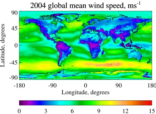
and R_dd are the same. The global mean wind speed for 2004, sampled at AATSR overpass times, is shown in Fig. 3. For wind speeds of approximately 10 ms−1 and higherf_wcandf_wcρ_wcare considerable (10−3₋10−2, except at 1.6 µm). Such high wind speeds are found polewards of 45◦, with typical ocean wind speeds elsewhere in the range 5–8 ms−1, corresponding toρ_wcaround 10−4₋10−3.

20

There are several sources of uncertainty with this section of the algorithm:

– There is a large uncertainty of up to 50% in the spectral reflectance of whitecaps (Frouin et al., 1996, Nicolas et al., 2001, Kokhanovsky, 2004).

– Anguelova and Webster (2006) reveal that diff_{erent parameterisations of}_f

wc can

lead to estimates diff_{ering by up to an order of magnitude, as a simple} depen-25

(15)

AMTD

3, 1023–1098, 2010

(A)ATSR

A. M. Sayer et al.

◭ ◮

5 Glint reflectance

The contributionρ_gl results from rays of light striking the sea surface and being spec-ularly reflected in the observer’s direction. It is calculated using the Fresnel equations, modified to account for the roughness of the wind-ruffl_{ed sea surface according to} statistics described by Cox and Munk (1954a) and Cox and Munk (1954b). More com-5

plicated than whitecaps, glint depends strongly on geometry, wind speed and wind direction, and weakly on wavelength.

5.1 Calculation

5.1.1 Slope distribution

The algorithm defines a coordinate system (P,X,Y,Z) such that P is the observed 10

point on the surface and Z the altitude with P Y in the direction of the Sun and P X

in the direction perpendicular to the Sun’s plane. The surface slope is defined by the following two components:

Z_x=∂Z

∂X =sinαtanβ (7)

Z_y=∂Z

∂Y =cosαtanβ (8)

15

In the aboveα is the azimuth of the ascent (clockwise from the Sun) andβthe tilt. Zx

andZ_y are related to the incident and reflected directions as follows, where θ_s< π/2 andθ_v>0:

Z_x= −sinθvsinφ cosθ_s+_cos_θ

v

(9)

Z_y=sinθs +_sin_θ

vcosφ

cosθ_s+_cos_θ

v

(16)

AMTD

3, 1023–1098, 2010

(A)ATSR

A. M. Sayer et al.

◭ ◮

Printer-friendly Version Interactive Discussion In reality, the slope distribution will be anisotropic and dependent on wind direction

χw. The axes are rotated clockwise from the north by χw to define a new coordinate

system (P,X′,Y′,Z) where P Y′ is parallel to the wind direction, and where the slope components may be re-expressed:

Z_x′=_cos(_χ

w)Zx+sin(χw)Zy (11)

5

Z_y′=₋_sin(_χ

w)Zx+cos(χw)Zy (12)

Following Cox and Munk (1954a), the probability distribution of surface facets

p(Z_x′,Z_y′) is required to calculate the glint reflectance. The original work provided coef-ficients for 3 parametrisations forp:

– Wind-isotropic (dependent only on absolute wind speed). 10

– Wind-anisotropic (dependent on upwind and crosswind wind speed).

– Wind-anisotropic, with an additional Gram-Charlier series correction term.

Recently, Zhang and Wang (2009) evaluated these parametrisations, along with other work drawing on the heritage of Cox and Munk (1954a) (specifically Wu, 1972; Mer-melstein et al., 1994; Shaw and Churnside, 1997; Shifrin, 2001; Ebuchi and Kizu, 15

2002, and Br ´eon and Henriot, 2006) using MODIS measurements. It was found that the anisotropic model (without the Gram-Charlier series) of Cox and Munk (1954a), and the model of Br ´eon and Henriot (2006), were very similar and provided the best model for the observed glint. The conclusions remain valid for (A)ATSR as it has sim-ilar channels to MODIS. Therefore the anisotropic model of Cox and Munk (1954a) is 20

(17)

AMTD

3, 1023–1098, 2010

(A)ATSR

A. M. Sayer et al.

◭ ◮

Printer-friendly Version Interactive Discussion that the peak of the glint be well-represented. The resulting expression for the slope

distribution is

p(Z_x′,Z_y′)= 1 2πσ′_xσ′_ye

(−ζ2+2η2) (13)

where the terms ζ=_Z′

x/σ′x and η=Zy′/σ′y, and σ′x and σ′y are the root mean square

values ofZ_x′andZ_y′respectively. The valuesσ′_x2, taken as as 0.003+_0.00192w_±_0.002, 5

and σ′y2, taken as 0.00316w±0.004, are from Cox and Munk (1954a) for a clean sea

surface.

5.1.2 The Fresnel reflection coe_fficient

The Fresnel reflection coeffi_cient_R

f describes the proportion of light hitting the surface

at some angle of incidenceΘ_{reflected at the same angle to the surface normal. The} 10

angle of the beam refracted into the water isΘ′_{; Snell’s Law describes the relationship} between these angles:

n_asinΘ =_n

wsinΘ′ (14)

The real component of the refractive index of air,n_a, is taken as 1.00029 for all wave-lengths. For water, real components of refractive indices were calculated at 550 nm and 15

670 nm using the method of Quan and Fry (1995) assuming a typical temperature of 15◦C and salinity of 35 parts per thousand, but are correct to four significant figures over the range of typical temperatures and salinities.

This model extends only to 700 nm, so for the longer wavelengths values for pure water from Hale and Querry (1973) were used. At shorter wavelengths there was an 20

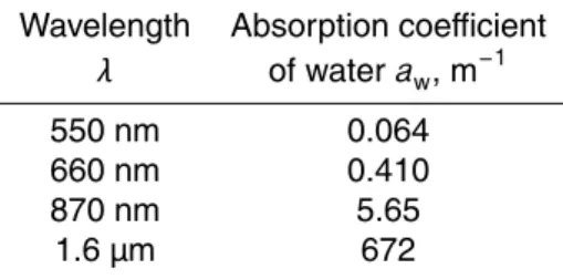
off_{set of around 0.0065 between the refractive index as predicted for pure water and} that of salinity typical for the sea, so this adjustment was also applied to the pure water data used at 870 nm and 1.6 µm. Values for the imaginary part of the refractive index were likewise taken from Hale and Querry (1973). The final data used are shown in Table 3.

(18)

AMTD

3, 1023–1098, 2010

(A)ATSR

A. M. Sayer et al.

◭ ◮

Printer-friendly Version Interactive Discussion The angleΘ_{can be calculated from Eqs. (7), (8), (9) and (10), and is described in}

theα andβcoordinate system by Cox and Munk (1954a). The following result can be obtained in terms of the known valuesθ_sandθ_v, which indirectly providesΘ_:

cos2Θ =_cos_θ

vcosθs+sinθvsinθscosφr (15)

Cox and Munk (1954a) and this work computeR_f neglecting the complex part of the 5

index of refraction (a valid approximation because this is a small term, as shown in Table 3). For unpolarised light,R_fis calculated as

Rf(Θ)=

1 2

_sin(_Θ

−Θ′₎ sin(Θ + Θ′₎

2 +

_tan(_Θ

−Θ′₎ tan(Θ + Θ′₎

2!

(16)

whereΘ′ _{is obtained from Eq. (14).}

5.1.3 Combination of terms

10

The total contributionρ_gl is calculated, following Cox and Munk (1954a), as

ρ_gl= πp(Z

′

x,Zy′)Rf

4cosθ_scosθ_vcos4_β (17)

where the facet tiltβmay be calculated from:

cosβ=cosθs

+_cos_θ

v

√

2+_2cos2Θ

(18)

For viewing zenith angles more extreme than 70◦, a slight modification is made to 15

Eq. (17) following Zeisse (1995):

ρ_gl= πp(Z

′

x,Zy′)Rf

(19)

AMTD

3, 1023–1098, 2010

(A)ATSR

A. M. Sayer et al.

◭ ◮

Printer-friendly Version Interactive Discussion The term B/A, known as the area of the ergodic cap, arises as a replacement to

cosθ_v to avoid an infinite radiance at viewing zenith angles near the ocean horizon. The reader is referred to Zeisse (1995) for more details; although such extreme viewing geometries do not occur for the (A)ATSR views, calculation of the reflectance at such geometries is required for the integration to obtainR_bdandR_ddfor the retrieval forward 5

model.

5.2 Magnitude of contribution

The glint contributionρ_gl toR_bb is shown at 550 nm in Fig. 4. The strong geometric dependence is visible; this is key to the ability of (A)ATSR to perform retrievals into the sun-glint region, as generally while one view is aff_{ected by glint (meaning most signal} 10

arises from the surface) the other is not (so most signal arises from the atmosphere). The asymmetry in Fig. 4 arises due to the wind direction not being in line with the field of view. This has a smaller impact as θ_v tends to the nadir. Dependence on wavelength is weak due to the similarity of the refractive index of water at the modelled wavelengths.

15

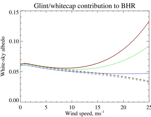
The sea surface BRDF is integrated using Gaussian quadrature with 4 points to obtainR_bdandR_dd. The glint contribution requires a large number of points to calculate accurately; as a result precalculated lookup tables (LUTs) of integratedρ_gl, using 360 quadrature points, are used for computational effi_{ciency. These are parametrised in} terms of wind speed (forR_dd) and wind speed and solar zenith angle (forR_bd). These 20

quantities are shown in Figs. 5 and 6. The glint DHR shows the expected increase with solar zenith angle, and for commonly-encountered conditions is approximately 0.03 (at all wavelengths; shown only for 550 nm). For high wind speeds the contribution decreases due to the increased whitecap fraction. The BHR is generally 0.05–0.06, decreasing asw increases again due to the increase in whitecap fraction. When the 25

(20)

AMTD

3, 1023–1098, 2010

(A)ATSR

A. M. Sayer et al.

◭ ◮

5.3 Uncertainties

Over a range of typical conditions, the uncertainties in the coeffi_{cients used in the} calculation ofp(Z_x′,Z_y′) (Eq. 13) lead to a variability of around 10%, causing a corre-sponding uncertainty inρ_gl of the same amount. This variability decreases at higher wind speeds.

5

6 Underlight

Underlight is upwelling irradiance from just below the surface of the ocean. As such,ρ_ul

is influenced strongly by pigment concentration and wavelength, and weakly by geom-etry. The model described here is designed for Case I waters, following the nomencla-ture of Morel and Prieur (1977). In Case I waters (typically open ocean) the chlorophyll 10

concentration is high compared to the scattering coeffi_{cient; in Case II waters (typically} coastal and shallow) scattering by inorganic particles dominates. The semi-empirical relationships between ocean constituents and surface reflectance developed by Morel and Prieur (1977), Morel and Gentili (1991) and later work are diff_{erent between Case I} and II waters. This work focusses on Case I waters because they cover the majority of 15

the Earth’s surface, and scattering in Case II waters is less well-understood.

6.1 Calculation

The underlight reflectance is an analogue to the atmospheric scattering problem. Re-flectances and transmittances related to underlight are denoted using_Rand_T, rather than R and T, for an easier distinction between other reflectance and transmittance 20

terms used in this work. Fundamentally, the system may be considered to consist of three layers:

(21)

AMTD

3, 1023–1098, 2010

(A)ATSR

A. M. Sayer et al.

◭ ◮

Printer-friendly Version Interactive Discussion the (downward) reflectance of upwelling irradiance below the interface is_R_u. The

upward reflectance of downwelling irradiance above the interface is the glint.

– An “upper ocean” layer, from which the scattered radiation causing the underlight contribution originates. The reflectance of this layer is denoted by_R_wand known as the water body reflectance.

5

– An “ocean floor” layer. This is characterised by the reflectance of the ocean bed,

Rbed. The transmittance between the upper layer and ocean floor is denotedTw,d

or_T_w_,_ufor downward and upward directions respectively.

The problem may be simplified by first considering a combination of the lower two layers. Light penetrating the air-water interface may be reflected back towards it (_R_w) 10

or subject to multiple “reflections” between the upper ocean and ocean floor. If it is assumed that _R_bed is isotropic then it can be easily shown that the combination of these two layers reduces to

Rw+

Tw,dRbedTw,u

1_−R_w_R_bed (20)

which is the reflectance_R_w of the incident light from the water body, plus a multiple-15

scattering geometric series limit.

This combination of the two lower layers may then be treated as a single (lower) layer of a two-layer system, in which the upper layer corresponds to the air-water interface. If it is assumed that this lower layer is an isotropic reflector then the same series limit may be applied to this simpler two-layer system to calculateρ_ul:

20

ρul=

Td(Rw+Tw,d

R_bedTw,u

1−RwRbed )Tu

1_−R_u(_R_w+Tw,dRbedTw,u

1−RwRbed )

(21)

(22)

AMTD

3, 1023–1098, 2010

(A)ATSR

A. M. Sayer et al.

◭ ◮

Printer-friendly Version Interactive Discussion off_{the interface was dealt with as the sun-glint term and so is not part of Eq. (21). A}

further approximation may be made to simplify the calculation ofρ_ulfor the open ocean. The transmittance_T_wof water (either upward or downward) may be calculated as

Tw=e−awz (22)

wherea_wis the absorption coeffi_{cient of the water, and}_z_{the path length (for a vertical} 5

column, equal to the depth of the water). For pure water,a_wcan be calculated from the complex part of the refractive index:

aw=

4π

λ κ (23)

Values of κ were tabulated in Table 3 and, assuming pure water, may be used to calculatea_wand hence_T_wfor a variety of depths. Over all wavelengths of interest, and 10

even in shallow water (withz=_{100 m),}_T

w is very small (with a maximum of 10−2 for

z=_{100 m at 550 nm, and orders of magnitude smaller for deeper water or longer} wave-lengths). These calculations are for pure water, and substances in seawater would fur-ther decrease_T_w. As a result_T_w_,_dR_bed_T_w_,_u, the proportion of light transmitted through the water, reflected off_{the bottom and then transmitted up through the water body, may} 15

be neglected as almost zero. Hence Eq. (21) may be simplified to

ρ_ul= TdRwTu

1_−R_u_R_w (24)

which is the expression used to calculateρ_ul in this scheme. It is noteworthy that in very shallow waters, or wavelengths at which water is more transparent, the reflectance characteristics of the ocean floor may become important. An analagous formulation 20

was presented by Austin (1974).

6.1.1 Downwelling transmittance coe_fficient,T_d

(23)

AMTD

3, 1023–1098, 2010

(A)ATSR

A. M. Sayer et al.

◭ ◮

Printer-friendly Version Interactive Discussion together with Eq. 14) for an incident beam of a given solar zenith angle, and noting that

light not reflected is transmitted:

Td(θs)=1−Rf:aw(θs) (25)

The subscript in _R_f:aw reminds that the incident beam is coming from the air, into the water. For all wavelengths,_T_d is approximately 0.98 forθ_s<60◦ but drops sharply 5

for larger zenith angles. Calculation for a wind-roughened sea is computationally ex-pensive, as it involves the calculation of the transmittance through all possible facets. Austin (1974) present results for selected angles and wind speeds, and note that for wind-ruffl_{ed seas}_T

dis slightly lower than 0.98 for near-zenith angles of incidence, and

the decline in transmittance is slower as the Sun approaches the horizon, although 10

the changes are not large. Therefore the assumption of a flat sea surface introduces minimal additional error.

6.1.2 Upwelling transmittance coefficient,T

u

The transmittance of the underlight through the water-air interface is denoted_T_u. If the upwelling irradiance is assumed to be diff_{use, and the sea surface flat, then}_T

uis given

15

by using the Fresnel equation and Snell’s Law (Eqs. 16 and 14) to integrate over all possible upwelling anglesθ_u:

Tu=

Rπ/2

0 (1−Rf:wa(θu))cosθusinθudθu

Rπ/2

0 cosθusinθudθu

(26)

Here,_R_f:waindicates that the upwelling light is travelling from water to air. The result-ing values of_T_uare 0.522 at 550 nm, 0.523 at 660 nm, 0.525 at 870 nm and 0.536 at 20

1.6 µm. These are just over half typical values of_T_d because rays hitting the interface withΘ_>_sin−1₍_n

a/nw), approximately 48◦, are internally reflected so that their energy

(24)

AMTD

3, 1023–1098, 2010

(A)ATSR

A. M. Sayer et al.

◭ ◮

Printer-friendly Version Interactive Discussion As with _T_d, for a rough sea calculation becomes more complicated because the

transmittance of facets aligned at diff_{erent angles to the surface has to be taken into} account. Austin (1974) again show, using examples at selected wind speeds and an-gles, that for increasingly rough seas the transmittance from upwelling rays at near-nadir indidence falls while some transmittance is possible for rays at angles larger than 5

the flat-sea critical angle. The net eff_{ect is that} _T

u shows little dependence on wind

speed, and so the flat-sea assumption is again valid.

6.1.3 Upwelling reflectance coefficient,R_u

The final geometric term _R_u is the (downward) reflectance coeffi_{cient for upwelling} radiance at the water-air boundary. This can be calculated as 1_{− T}_u. Austin (1974) 10

give broadband visible values between 0.485 for a still ocean surface and 0.463 for a wind-ruffl_{ed surface with}_w=_{16 ms}−1_{; as this dependence on wind speed is small, and}

RuRw≪1, the flat-surface assumption introduces negligible error into Eq. (24).

6.1.4 Water body reflectance,R_w

The water body reflectance _R_w is controlled by the optical properties of water and 15

matter within it, and is defined as the ratio of upwelling irradiance from just below the surfaceE_u(λ) to downwelling irradiance just above itE_d(λ):

Rw=

E_u(λ)

Ed(λ)

(27)

The method of calculation is based on the method of in Morel and Prieur (1977), and further developed on many occasions (e.g. in Morel, 1988 or Morel and Gentili, 1991). 20

The parametrisations are based on a variety of semiempirical relationships. The water body reflectance is calculated from the optical properties of the water as follows:

Rw=f

b_b(λ)

(25)

AMTD

3, 1023–1098, 2010

(A)ATSR

A. M. Sayer et al.

◭ ◮

Printer-friendly Version Interactive Discussion This describes the colour of the water as the ratio of the total backscattering

coef-ficientb_b(λ) to the absorption coeffi_cient_a₍_λ_{), multiplied by some empirical correction} factorf.

6.1.5 Absorption coefficient

A more thorough treatment can be given to the absorption coeffi_{cient of water than the} 5

approximation made previously. The total absorption coeffi_cient_a _{of seawater can be} thought of as the sum of the absorption due to pure water,a_w (as in Eq. 23), that due to phytoplankton pigmentsa_ph, anda_CDOM, the absorption due to detritus and coloured dissolved organic matter (CDOM), also known asGelbstoff:

a(λ)=_a

w(λ)+aph(λ)+aCDOM(λ) (29)

10

The absorption coeffi_{cients used for water are shown in Table 4. Values for 550 nm} and 660 nm are taken for seawater from Morel and Prieur (1977); for longer wave-lengths data are unavailable so at 870 nm and 1.6 µma_wis estimated using imaginary components of the refractive index from Table 3 with Eq. (23). Use of this approximation is justified as the underlight contribution to_R_bbis small at these wavelengths.

15

Fora_ph, the two-component model outlined by Sathyendranath et al. (2001) is used, with coeffi_{cients from analysis of multiple measurement campaigns in di}ff_{erent regions} as described by Devred et al. (2006). This relates the absorption due to phytoplankton to the concentrationCof chlorophyll-ain mg m−3, assuming a mixed population of two phytoplankton types, by the following equation:

20

a_ph(λ)=_U₍₁₋_e−SchlC₎+_a∗

2(λ)C (30)

The parameterU is defined as

U(λ)=_Cm

1(a∗1(λ)−a∗2(λ)) (31)

(26)

AMTD

3, 1023–1098, 2010

(A)ATSR

A. M. Sayer et al.

◭ ◮

Printer-friendly Version Interactive Discussion (mg chl-a)−1 of the two populations at the wavelength of interest. S_chl describes the

nonlinearity of absorption and has units of m3(mg chl-a)−1. For a global dataset, De-vred et al. (2006) found Cm₁ =₀_._{62 mg m}−3_, _a∗

1=0.0109 m− 1

(mg chl-a)−1 at 550 nm and 0.0173 m−1 (mg chl-a)−1 at 660 nm, a∗₂=₀_._{0064 m}−1 _{(mg chl-}_a₎−1 _{at 550 nm and} 0.0085 m−1 (mg chl-a)−1 at 660 nm, and S_chl=₁_._{61 m}3 _{(mg chl-}_a₎−1_{. Absorption by} 5

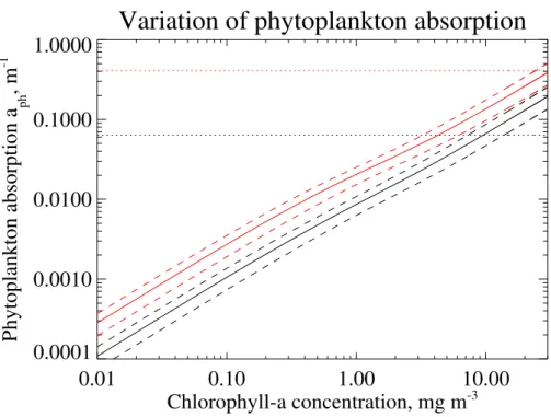
pigments is neglected at 870 nm and 1.6 µm; the very strong absorption of the water at these wavelengths (Table 4) means this approximation has negligible impact. This model results in the profile ofa_ph shown in Fig. 7. It is not appropriate to considera_ph

as simply the product of C and a reference pigment absorption coeffi_{cient, as} _a

ph is

observed to vary nonlinearly with C, due to dependencies on plankton cell size and 10

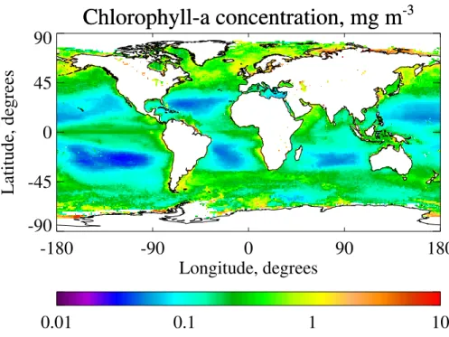
structure and the presence of accessory pigments (e.g. Fujiki and Taguchi, 2002). Operationally, data for both chlorophyll concentration and CDOM/detritus absorption are obtained from the GlobColour project (Barrot et al., 2006). This provides global values of various ocean colour parameters from merged satellite (MERIS, SeaWIFS and MODIS) datasets. Monthly mean values on an approximately 25 km_×25 km grid 15

are used, with gaps filled using an annual mean. Figure 8 shows the annual mean pigment (chlorophyll-a and phaeophytin-a, normally abbreviated as just “chlorophyll”) concentrations over 2004. The large spatial variability, as well as range of concen-trations spanning several orders of magnitude, is evident. In the open ocean, typical values are in the range 0.05 to 1 mg m−3 but near the coast the concentration can 20

reach 10 mg m−3 or higher. Chlorophyll content is also important for calculating the backscattering coeffi_{cient, as discussed in the next section.}

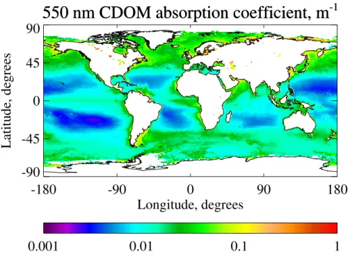
Figure 9 presents an analagous map of the annual mean CDOM absorption coeffi -cient at 550 nm for 2004. According to Roesler et al. (1989), absorption from detritus and CDOM can be treated as one parameter due to their similar spatial distributions 25

(27)

AMTD

3, 1023–1098, 2010

(A)ATSR

A. M. Sayer et al.

◭ ◮

Printer-friendly Version Interactive Discussion following equation:

a_CDOM(λ)=_a

CDOM(443)e−S(λ−443) (32)

In Eq. (32) the parameterS describes the spectral slope of the absorption. Roesler et al. (1989) found diff_{erent values (generally in the range 0.011 to 0.018) worked well} for diff_{erent regions of the world, with 0.014 a good value for global studies. This value} 5

of 0.014 is used here, as well as assorted other studies (such as Chen et al., 2003). The CDOM absorption coeffi_{cient tends to covary with chlorophyll concentration} (Figs. 8 and 9). Typical ocean values at 550 nm are in the range 0.001 to 0.01 m−1 but again higher values, generally up to 0.1 m−1, can be observed in productive or coastal waters. This algorithm only takesa_CDOMinto account at 550 nm. At 660 nm the 10

value ofS means that CDOM absorption is only around a fifth as strong as at 550 nm. Combined with the fact that absorption by water and chlorophyll increases by roughly an order of magnitude, the CDOM contribution to the total absorption coeffi_{cient is} neg-ligible. At longer wavelengths this eff_{ect is even more pronounced. Taking into account} the decreasing importance of ρ_ul with increasing wavelength, this approximation has 15

minimal eff_{ect on results.}

6.1.6 Backscattering coefficient

The termbb(λ) represents the total backscattering coefficient, defined after Morel and

Prieur (1977):

b_b(λ)=_b

bw(λ)+bbp(λ) (33)

20

This equation simply states that the total backscattering coeffi_cient _b

b is the sum of

backscattering due to molecules, b_bw, and particles, b_bp. These terms may be fur-ther parameterised; firstly, b_bw may be represented as b_w/2 (molecular scattering is forward-back symmetric so the backscatter coeffi_cient_b

bw is half of the molecular

scattering coeffi_cient_b

w). Secondly, in Case I waters scattering due to particles may

(28)

AMTD

3, 1023–1098, 2010

(A)ATSR

A. M. Sayer et al.

◭ ◮

Printer-friendly Version Interactive Discussion be regarded as the product of the particle backscattering probability ˜b_b and particle

backscattering coeffi_cient_b_{, leading to Eq. (34):}

b_b(λ)=1

2bw(λ)+b˜b(λ)b (34)

Values forb_wfor pure water from 380 nm to 700 nm were given by Morel and Prieur (1977). Morel (1974) tabulated values from 350 nm to 600 nm for both pure water 5

and typical seawater. The data were shown to fit a power law with a dependence on λ−4.32, with seawater scattering around 1.30 times as much as pure water. This relationship has been used to extrapolate these data to the 660 nm, 870 nm and 1.6 µm channels. The values obtained forb_ware 1.93_×10−3m−1at 550 nm, 8.77_×10−4m−1at 660 nm, 2.66_×10−4m−1at 870 nm and 1.91_×10−5m−1 at 1.6 µm. The value predicted 10

for 660 nm is in good agreement with that given for pure water at 660 nm in Morel and Prieur (1977) multiplied by 1.30. Another point to note is thatbw is generally small

(both in absolute terms and when compared to ˜b_b) at longer wavelengths, meaning any error in this extrapolation is minor in terms of influence on_R_w.

The second parameter in Eq. (33), ˜b_b(λ), is the backscattering probability: the ratio 15

of the backscattering to scattering coeffi_{cients of the pigments. It is related to the} total concentration C of chlorophyll a and pheophytin a, measured in mg m−3, and wavelengthλ, measured in nm, by the following expression:

˜

b_b(λ)=₀_.₀₀₂+₀_.₀₂₍₀_.₅₋₀_._25log

10C)

550

λ (35)

The final term in the backscatter component of Eq. (33),bis calculated as: 20

b=₀_.₃_C0.62 ₍₃₆₎

The relationship betweenb andCwas derived by Morel (1988) for data at 550 nm; the wavelength-dependence of particle backscattering is taken into account by theλ−1

factor in Eq. (35). It should be noted that although parametrised in terms of C, the models were developed to account for scattering from suspended organic matter as 25

(29)

AMTD

3, 1023–1098, 2010

(A)ATSR

A. M. Sayer et al.

◭ ◮

6.1.7 Ratio multiplierf and combination for water body reflectanceR_w

Morel and Prieur (1977) initially gavef, the empirical correction multiplier of the ratio of total backscattering to total absorption used to calculate the water body reflectance_R_w, a value of 0.33. Subsequent work has found it to depend on the solar geometry and the optical properties of water. The method used here was put forward by Morel and Gentili 5

(1991), stated to be accurate within 1.5% for solar zenith angles smaller than 70◦. It relatesf to the proportion of backscattering due to water molecules (ηb=bbw/bb) and

the cosine of the solar zenith angle (µ_s) as follows:

f=₀_.₆₂₇₉₋₀_.₂₂₂₇_η

b−0.0513η2_b+(−0.3119+0.2465ηb)µs (37)

Assuming a pigment concentration of 0.3 mg m−3, representative η_bvalues are ap-10

proximately 0.32 at 550 nm, 0.20 at 660 nm, 0.09 at 870 nm and 0.01 at 1.6 µm. The corresponding variation off is small with wavelength but larger with solar angle, from slightly over 0.3 for a near-nadir sun to over 0.5 for a sun near the horizon. The older constant value of 0.33 forf would in most cases be an underestimate.

6.2 Magnitude of contribution

15

Figure 10 shows ρ_ul at (A)ATSR wavelengths for a range of representative pigment concentrations. At the shorter wavelengths it is of the order of 10−2₋10−3, and so away from the glint region is generally equal to or larger than other contributions to

R_bb. Hence knowledge of Cis essential to judge accurately the total reflectance. As it shows a stronger wavelength-dependence than ρ_wc and ρ_gl, the spectral shape of 20

Rbb will be largely determined by ρul outside of the sun-glint region. At 870 nm and

1.6µm, ρ_ul is negligible. At all wavelengthsρ_ul increases with C, although at 550 nm

(30)

AMTD

3, 1023–1098, 2010

(A)ATSR

A. M. Sayer et al.

◭ ◮

6.3 Uncertainties

The major uncertainties associated withρ_ul are errors arising from poor characterisa-tion of pigment and CDOM distribucharacterisa-tions and scattering. The small size of the underlight term at the longer two wavelengths means that errors inρ_ulwill only have minor impacts on the modelled reflectance at 550 nm and 660 nm.

5

– The relationship between ˜b_bandCwas developed for Case I waters (according to the definitions of Morel and Prieur, 1977) and so may not accurately characterise scattering in Case II waters (where pigment and scattering particles do not covary in the same way). This may cause the algorithm to perform less well over Case II waters. Case II waters are largely coastal and the inhomogeneity of coastal re-10

gions presents other problems for aerosol retrieval; this is beyond the scope of this work.

– Errors arising from use of monthly means for chlorophyll and CDOM values. The GlobColour chlorophyll products have a stated accuracy of 31%. CDOM errors are not given by Barrot et al. (2006). Further errors arise due to variations on 15

shorter timescales than a month.

– There may be regional biases from using 0.014 as a global CDOM spectral slope

S, as Roesler et al. (1989) found values from 0.011 to 0.018 in diff_{erent parts of} the world.

– Neglecting CDOM and detritus absorption at wavelengths longer than 550 nm 20