ROUGH SET AND RULE-BASED MULTICRITERIA DECISION AIDING*
Roman Slowinski
1**, Salvatore Greco
2and Benedetto Matarazzo
2Received June 30, 2012 / Accepted July 28, 2012
ABSTRACT.The aim of multicriteria decision aiding is to give the decision maker a recommendation concerning a set of objects evaluated from multiple points of view called criteria. Since a rational decision maker acts with respect to his/her value system, in order to recommend the most-preferred decision, one must identify decision maker’s preferences. In this paper, we focus on preference discovery from data concerning some past decisions of the decision maker. We consider the preference model in the form of a set of “if..., then...” decision rules discovered from the data by inductive learning. To structure the data prior to induction of rules, we use the Dominance-based Rough Set Approach (DRSA). DRSA is a methodology for reasoning about data, which handles ordinal evaluations of objects on considered criteria and monotonic relationships between these evaluations and the decision. We review applications of DRSA to a large variety of multicriteria decision problems.
Keywords: multicriteria decision aiding, ordinal classification, choice, ranking, Dominance-based Rough Set Approach, preference modeling, decision rules.
1 INTRODUCTION
In this paper, we review a multicriteria decision aiding methodology which employs decision maker’s (DM’s) preference model in form of a set of decision rules discovered from some prefer-ence data. Multicriteria decision problems concern a finite set ofobjects(also called alternatives, actions, acts, solutions, etc.) evaluated by a finite set ofcriteria(also called attributes, features, variables, etc.), and raise one of the following questions: (i) how to assign the objects to some ordered classes (ordinal classification), (ii) how to choose the best subset of objects (choiceor
optimization), or (iii) how to rank the objects from the best to the worst (ranking). The answer to everyone of these questions involves an aggregation of the multicriteria evaluations of objects, which takes into account preferences of the DM. In consequence, the aggregation formula is at
*Invited paper **Corresponding author
1Institute of Computing Science, Poznan University of Technology, 60-965 Poznan, and Systems Research Institute, Polish Academy of Sciences, 01-447 Warsaw, Poland. E-mail: [email protected]
the same time the DM’spreference model. Thus, any recommendation referring to one of the above questions must be based on the DM’s preference model. The preference data used for building this model, as well as the way of building and using it in the decision process, are main factors distinguishing various multicriteria decision aiding methodologies.
In our case, we assume that thepreference dataincludes either observations of DM’s past deci-sions in the same decision problem, or examples of decideci-sions consciously elicited by the DM on demand of an analyst. This way of preference data elicitation is called indirect, by opposition todirectelicitation when the DM is supposed to provide information leading directly to defini-tion of all preference model parameters, like weights and discriminadefini-tion thresholds of criteria, trade-off rates, etc. (see,e.g., Roy, 1996).
Past decisions or decision examples may be, however,inconsistentwith the dominance principle commonly accepted for multicriteria decision problems. Decisions are inconsistent with the dominance principle if:
• in case of ordinal classification: objectahas been assigned to a worse decision class than objectb, althoughais at least as good asbon all the considered criteria,i.e. adominates
b;
• in case of choice and ranking: pair of objects(a,b)has been assigned a degree of pref-erence worse than pair(c,d), although differences of evaluations betweenaandbon all the considered criteria is at least as good as respective differences of evaluations between
candd,i.e.pair(a,b)dominates pair(c,d).
Thus, in order to build a preference model from partly inconsistent preference data, we had an idea to structure this data using the concept of arough setintroduced by Pawlak (1982, 1991). Since its conception, rough set theory has often proved to be an excellent mathematical tool for the analysis of inconsistent description of objects. Originally, its understanding of inconsistency was different, however, than the above inconsistency with the dominance principle. The original rough set philosophy is based on the assumption that with every object of the universeUthere is associated a certain amount of information (data, knowledge). This information can be ex-pressed by means of a number of attributes. The attributes describe the objects. Objects which have the same description are said to be indiscernible (or similar) with respect to the available information. Theindiscernibility relationthus generated constitutes the mathematical basis of rough set theory. It induces a partition of the universe into blocks of indiscernible objects, called elementary sets, which can be used to build knowledge about a real or abstract world. The use of the indiscernibility relation results in informationgranulation.
The difference between the upper and lower approximation constitutes the boundary region of the rough set, whose elements cannot be characterized with certainty as belonging or not to X
(by using the available information). The information about objects from the boundary region is, therefore, inconsistent or ambiguous. The cardinality of the boundary region states, moreover, the extent to which it is possible to expressXin exact terms, on the basis of the available informa-tion. For this reason, this cardinality may be used as a measure of vagueness of the information aboutX.
Some important characteristics of the rough set approach makes it a particularly interesting tool in a variety of problems and concrete applications. For example, it is possible to deal with both quantitative and qualitative input data and inconsistencies need not to be removed prior to the analysis. In terms of the output information, it is possible to acquirea posterioriinformation regarding the relevance of particular attributes and their subsets to the quality of approximation considered within the problem at hand. Moreover, the lower and upper approximations of a par-tition ofUinto decision classes, prepare the ground for inducingcertainandpossibleknowledge patterns in the form of “if... then...” decision rules.
Several attempts have been made to employ rough set theory for decision aiding (Slowinski, 1993; Pawlak & Slowinski, 1994). The Indiscernibility-based Rough Set Approach (IRSA) is not able, however, to deal with preference ordered attribute scales and preference ordered decision classes. In multicriteria decision analysis, an attribute with a preference ordered scale (value set) is called acriterion.
An extension of the IRSA which deals with inconsistencies with respect to dominance principle, typical for preference data, was proposed by Greco, Matarazzo & Slowinski (1998a, 1999a,b). This extension, called the Dominance-based Rough Set Approach (DRSA) is mainly based on the substitution of the indiscernibility relation by a dominance relation in the rough approximation of decision classes. An important consequence of this fact is the possibility of inferring (from observations of past decisions or from exemplary decisions) the DM’s preference model in terms of decision rules which are logical statements of the type “if..., then...”. The separation ofcertain
anduncertainknowledge about the DM’s preferences is carried out by the distinction of different kinds of decision rules, depending upon whether they are induced from lower approximations of decision classes or from the difference between upper and lower approximations (composed of inconsistent examples). Such a preference model is more general than the classical functional models considered within multi-attribute utility theory or the relational models considered, for example, in outranking methods (Grecoet al., 2002c, 2004; Slowinskiet al., 2002b).
DRSA with respect to multicriteria choice and ranking. In Sections 4 and 5, application of DRSA to all three categories of multicriteria decision problems is explained by the way of examples. Section 6 groups conclusions and characterizes other relevant extensions and applications of DRSA to decision problems. Finally, Section 7 provides information about additional sources of information about rough set theory and applications.
2 SOME BASICS ON INDISCERNIBILITY-BASED ROUGH SET APPROACH (IRSA)
2.1 Definition of rough approximations by IRSA
For algorithmic reasons, we supply the information regarding the objects in the form of a data table, whose separate rows refer to distinct objects and whose columns refer to the different attributes considered. Each cell of this table indicates an evaluation (quantitative or qualitative) of the object placed in that row by means of the attribute in the corresponding column.
Formally, adata tableis the 4-tupleS= hU,Q,V, fi, whereU is a finite set ofobjects (uni-verse), Q = {q1,q2, . . . ,qm}is a finite set ofattributes,Vq is the value set of the attributeq,
V = ∪q∈QVqand f :U×Q →V is a total function such that f(x,q)∈ Vqfor eachq ∈ Q,
x∈U, called theinformation function.
Each objectxofUis described by a vector (string)
DesQ(x)=f(x,q1), f(x,q2), . . . , f(x,qm),
called thedescriptionofxin terms of the evaluations of the attributes fromQ. It represents the available information aboutx.
To every (non-empty) subset of attributes P we associate anindiscernibility relationonU, de-noted byIPand defined as follows:
IP =(x,y)∈U×U : f(x,q)= f(y,q), for eachq∈ P .
If(x,y)∈ IP, we say that the objectsxandyareP-indiscernible. Clearly, the indiscernibility relation thus defined is an equivalence relation (reflexive, symmetric and transitive). The family of all the equivalence classes of the relation IP is denoted byU|IP and the equivalence class containing an objectx ∈Uis denoted by IP(x). The equivalence classes of the relationIP are called theP-elementary setsorgranules of knowledgeencoded by P.
LetS be a data table, X be a non-empty subset ofU and∅ 6= P ⊆ Q. The set X may be characterized by two ordinary sets, called the P-lower approximationof X (denoted byP(X)) and theP-upper approximationofX(denoted byP(X)) inS. They can be defined, respectively, as:
P(X)=x∈U: IP(x)⊆X , P(X)=x∈U: IP(x)∩X6=∅ .
P(X)are all and only those objectsx∈U which belong to the equivalence classes generated by the indiscernibility relation IPcontaining at least oneobjectxbelonging to X. In other words,
P(X)is the largest union of the P-elementary sets included in X, while P(X)is the smallest union of theP-elementary sets containing X.
The lower and upper approximations can be written in an equivalent form, in terms of unions of elementary sets as follows:
P(X)= [ x∈U,IP(x)⊆X
IP(x), P(X)=
[
x∈X
IP(x) .
TheP-boundaryof XinS, denoted byBnP(X), is defined as: BnP(X)=P(X)−P(X) .
The termrough approximationis a general term used to express the operation of the P-lower andP-upper approximation of a set or of a union of sets. The rough approximations obey the following basic laws (cf. Pawlak, 1991):
• the inclusion property: P(X)⊆X ⊆P(X),
• the complementarity property: P(X)=U−P(U−X).
Directly from the definitions, we can also get the following properties of the P-lower and P -upper approximations (Pawlak, 1982, 1991):
1) P(∅)=P(∅), P(U)=P(U)=U, 2) P(X∪Y)=P(X)∪P(Y),
3) P(X∩Y)=P(X)∩P(Y), 4) X ⊆Y ⇒ P(X)⊆P(Y), 5) X ⊆Y ⇒ P(X)⊆P(Y), 6) P(X∪Y)⊇P(X)∪P(Y), 7) P(X∩Y)⊆P(X)∩P(Y), 8) P(P(X))=P(P(X))=P(X), 9) P(P(X))=P(P(X))=P(X).
If theP-boundary ofXis empty (i.e. BnP(X)=∅) then the setX is an ordinary set, called the
P-exact set. By this, we mean that it may be expressed as the union of some P-elementary sets. Otherwise, ifBnP(X)6=∅, then the setXis a P-rough set and may be characterized by means of P(X)andP(X).
The following ratio defines anaccuracymeasure of the approximation of X(X 6=∅)by means of the attributes from P: αP(X)= |P(X)|
|P(X)|, where|Y|denotes the cardinality of a (finite) setY.
Obviously, 0≤αP(X)≤1. IfαP(X)=1, thenX is aP-exact set. IfαP(X) <1, thenX is a
P-rough set.
Another ratio defines a qualitymeasure of the approximation of X by means of the attributes from P: γP(X) = |P|(XX|)|. The qualityγP(X)represents the relative frequency of the objects correctly assigned by means of the attributes from P. Moreover, 0≤αP(X)≤γP(X)≤1, and
γP(X)=0 iffαP(X)=0, whileγP(X)=1 iffαP(X)=1.
The definition of approximations of a subsetX ⊆Ucan be extended to a classification,i.e.a par-titionY = {Y1, . . . ,Yn}ofU. The subsetsYi,i =1, . . . ,n, are disjunctive classes ofY. By the
P-lower and P-upper approximations ofY inS we mean the setsP(Y)= {P(Y1), . . . ,P(Yn)} and P(Y) = {P(Y1), . . . ,P(Yn)}, respectively. The coefficientγP(Y) =
Pn
i=1|P(Yi)|
|U| is called
thequality of approximation of classification Y by the set of attributes P, or in short, thequality of classification. It expresses the ratio of all P-correctly classified objects to all objects in the data table.
The main issue in rough set theory is the approximation of subsets or partitions of U, repre-sentingknowledgeaboutU, with other sets or partitions that have been built up using available information aboutU. From the perspective of a particular objectx ∈U, it may be interesting, however, to use the available information to assess the degree of its membership to a subset Xof
U. The subsetX can be identified with the knowledge to be approximated. Using the rough set approach one can calculate the membership functionµPX(x)(rough membership function) as
µPX(x)= |X∩IP(x)| |IP(x)|
The value ofµPX(x)may be interpreted analogously as conditional probability and may be un-derstood as thedegree of certainty(credibility) to whichxbelongs toX. Observe that the value of the membership function is calculated from the available data, and not subjectively assumed, as it is in the case of membership functions of fuzzy sets.
Between the rough membership function and the rough approximations of Xthe following rela-tionships hold:
P(X)=x∈U :µXP(x)=1 , P(X)=x∈U :µPX(x) >0 ,
BnP(X)=x∈U:0< µPX(x) <1 , P(U−X)=
x∈U :µPX(x)=0 .
A very important concept for concrete applications is that of the dependence of attributes. Intu-itively, a set of attributesT ⊆Q totally dependsupon a set of attributes P ⊆Qif all the values of the attributes fromT are uniquely determined by the values of the attributes fromP. In other words, this is the case if a functional dependence exists between evaluations by the attributes from P and by the attributes from T. This means that the partition (granularity) generated by the attributes fromP is at least as “fine” as that generated by the attributes fromT, so that it is sufficient to use the attributes fromPto build the partitionU|IT. Formally,T totally depends on
PiffIP ⊆IT.
Therefore,T is totally (partially) dependent onPif all (some) objects of the universeUmay be univocally assigned to granules of the partitionU|IT, using only the attributes fromP.
Another issue of great practical importance is that ofknowledge reduction. This concerns the elimination of superfluous data from the data table, without deteriorating the information con-tained in the original table.
LetP ⊆Qandp∈ P. It is said that attribute pissuperfluousinP ifIP =IP−{p}; otherwise, pisindispensableinP.
The setPisindependentif all its attributes are indispensable. The subsetP′of Pis areductof
P(denoted byR E D(P)) ifP′is independent andIP′ =IP.
A reduct of P may also be defined with respect to an approximation of the classificationY of objects fromU. It is then called a Y -reductof P (denoted by R E DY(P)) and it specifies a minimal (with respect to inclusion) subset P′of P which keeps the quality of the classification unchanged,i.e.γP′(Y)=γP(Y). In other words, the attributes that do not belong to aY-reduct
ofPare superfluous with respect to the classificationY of objects fromU.
More than oneY-reduct (or reduct) of P may exist in a data table. The set containing all the indispensable attributes of P is known as the Y -core (denoted by C O R EY(P)). In formal terms,C O R EY(P) = ∩R E DY(P). Obviously, since the Y-core is the intersection of all the
Y-reducts of P, it is included in every Y-reduct of P. It is the most important subset of at-tributes ofQ, because none of its elements can be removed without deteriorating the quality of the classification.
2.2 Decision rules induced from rough approximations
In a data table the attributes of the setQare often divided intoconditionattributes (setC6=∅) anddecisionattributes (setD6=∅). Note thatC∪D=QandC∩D=∅. Such a table is called adecision table. The decision attributes induce a partition ofUdeduced from the indiscernibility relationIDin a way that is independent of the condition attributes. D-elementary sets are called
Since the tendency is to underline the functional dependencies between condition and decision attributes, a decision table may also be seen as a set ofdecision rules. These are logical state-ments of the type “if..., then...”, where the antecedent (condition part) specifies values assumed by one or more condition attributes (describing C-elementary sets) and the consequence (de-cision part) specifies an assignment to one or more de(de-cision classes (describing D-elementary sets). Therefore, the syntax of a rule can be outlined as follows:
if f(x,q1)is equal torq1and f(x,q2)is equal torq2and... f(x,qp)is equal torq p, thenxbelongs toYj1orYj2or. . .Yj k,
where{q1,q2, . . . ,qp} ⊆C, (rq1,rq2, . . . ,rq p)∈Vq1×Vq2× ∙ ∙ ∙ ×Vq pandYj1,Yj2, . . . ,Yj k are some decision classes of the considered classification (D-elementary sets). If there is only one possible consequence,i.e. k=1, then the rule is said to becertain, otherwise it is said to be
approximateorambiguous.
An objectx ∈U supportsdecision ruler if its description is matching both the condition part and the decision part of the rule. We also say that decision ruler coversobjectx if it matches at least the condition part of the rule. Each decision rule is characterized by itsstrengthdefined as the number of objects supporting the rule. In the case of approximate rules, the strength is calculated for each possible decision class separately.
Let us observe that certain rules are supported only by objects from the lower approximation of the corresponding decision class. Approximate rules are supported, in turn, only by objects from the boundaries of the corresponding decision classes.
Procedures for the generation of decision rules from a decision table use aninductive learning
principle. The objects are considered as examples of decisions. In order to induce decision rules with a unique consequent assignment to a D-elementary set, the examples belonging to the D -elementary set are called positive and all the othersnegative. A decision rule isdiscriminant
if it is consistent (i.e. if it distinguishes positive examples from negative ones) and minimal
(i.e. if removing any attribute from a condition part gives a rule covering negative objects). It may be also interesting to look forpartly discriminantrules. These are rules that, besides positive examples, could cover a limited number of negative ones. They are characterized by a coefficient, called thelevel of confidence, which is the ratio of the number of positive examples (supporting the rule) to the number of all examples covered by the rule.
The generation of decision rules from decision tables is a complex task and a number of proce-dures have been proposed to solve it (see, for example, Grzymala-Busse, 1992, 1997; Skowron, 1993; Ziarko & Shan, 1994; Skowron & Polkowski, 1997; Stefanowski, 1998; Slowinski, Ste-fanowski, Greco & Matarazzo, 2000). The existing induction algorithms use one of the following strategies:
(a) The generation of a minimal set of rules covering all objects from a decision table.
(c) The generation of a set of ‘strong’ decision rules, even partly discriminant, covering rela-tively many objects from the decision table (but not necessarily all of them).
To summarize the above description of IRSA, let us list particular benefits one can get when applying the rough set approach to analysis of data presented in decision tables:
• a characterization of decision classes in terms of chosen attributes through lower and upper approximation,
• a measure of the quality of approximation which indicates how good the chosen set of attributes is for approximation of the classification,
• a reduction of the knowledge contained in the table to a description by relevant attributes
i.e. those belonging to reducts; at the same time, exchangeable and superfluous attributes are also identified,
• a core of attributes, being an intersection of all reducts, indicates indispensable attributes,
• a set of decision rules which is induced from the lower and upper approximations of the decision classes; this shows classification patterns which exist in the data set.
A tutorial example illustrating all these benefits has been given in (Slowinskiet al., 2005). For more details about IRSA and its extensions, the reader is referred to Pawlak (1991), Polkowski (2002), Slowinski (1992b) and many others (see Section 7). Internet addresses to freely available software implementations of these algorithms can also be found in the last section of this paper.
2.3 From indiscernibility to similarity
As mentioned above, the classical definitions of lower and upper approximations are based on the use of the binary indiscernibility relation which is an equivalence relation. The indiscernibility implies the impossibility of distinguishing between two objects ofU having thesame descrip-tion in terms of the attributes from Q. This relation induces equivalence classes onU, which constitute the basic granules of knowledge. In reality, due to the imprecision of data describing the objects, small differences are often not considered significant for the purpose of discrimina-tion. This situation may be formally modeled by considering similarity or tolerance relations (see
e.g. Nieminen, 1988; Marcus, 1994; Slowinski, 1992a; Polkowski, Skowron & Zytkow, 1995; Skowron & Stepaniuk, 1995; Slowinski & Vanderpooten, 1995, 2000; Stepaniuk, 2000; Yao & Wong, 1995).
Replacing the indiscernibility relation by a weaker binarysimilarityrelation has considerably extended the capacity of the rough set approach. This is because, in the least demanding case, the similarity relation requires reflexivity only, relaxing the assumptions of symmetry and transitivity of the indiscernibility relation.
precisely, the similarity class of x, denoted by R(x), consists of the set of objects which are similar tox:
R(x)= {y∈U: y Rx}.
It is obvious that an object y may be similar to both x andz, while z is not similar tox,i.e. y∈ R(x)andy∈ R(z), butz∈/ R(x),x,y,z∈U. The similarity relation is of course reflexive (each object is similar to itself). Slowinski & Vanderpooten (1995, 2000) have proposed a simi-larityrelation which is onlyreflexive. The abandonment of the transitivity requirement is easily justifiable. For example, see Luce’s paradox of the cups of tea (Luce, 1956). As for the symme-try, one should notice thaty Rx, which means “yis similar tox”, is directional. There is a subject
yand a referentx, and in general this is not equivalent to the proposition “xis similar to y”, as maintained by Tversky (1977). This is quite immediate when the similarity relation is defined in terms of a percentage difference between evaluations of the objects compared on a numeri-cal attribute in hand, numeri-calculated with respect to evaluation of the referent object. Therefore, the symmetry of the similarity relation should not be imposed. It then makes sense to consider the inverse relation of R, denoted byR−1, wherex R−1ymeans again “yis similar tox”. R−1(x),
x∈U, is the class of referent objects to whichxis similar:
R−1(x)= {y∈U:x R y}.
Given a subset X ⊆ U and a similarity relation R onU, an objectx ∈ U is said to be non-ambiguousin each of the two following cases:
• xbelongs to X without ambiguity, that isx ∈ Xand R−1(x)⊆ X; such objects are also calledpositive;
• x does not belong to X without ambiguity (xclearly does not belong to X), that isx ∈
U−XandR−1(x)⊆U−X(orR−1(x)∩X 6=∅); such objects are also callednegative.
The objects which are neither positive nor negative are said to be ambiguous. A more general definition of lower and upper approximation may thus be offered (see Slowinski & Vanderpooten, 2000). LetX ⊆Uand letRbe a reflexive binary relation defined onU. The lower approximation of X, denoted by R(X), and the upper approximation of X, denoted by R(X), are defined, respectively, as:
R(X)=x∈U :R−1(x)⊆X ,
R(X)= [ x∈X
R(x) .
It may be demonstrated that the key properties – inclusion and complementarity – still hold and that
R(X)=
x∈U :R−1(x)∩X 6=∅ .
(upper approximation) when a similarity relation is reflexive, but not necessarily symmetric nor transitive.
Using a similarity relation, we are able to induce decision rules from a decision table. The syntax of a rule is represented as follows:
If f(x,q1)is similar torq1and f(x,q2)is similar torq2and... f(x,qp)is similar torq p, thenxbelongs toYj1orYj2or...Yj k,
where{q1,q2, . . . ,qp} ⊆C,(rq1,rq2, . . . ,rq p)∈Vq1×Vq2×. . .×Vq pandYj1,Yj2, . . . ,Yj k are some classes of the considered classification (D-elementary sets). As mentioned above, if
k=1 then the rule iscertain, otherwise it isapproximateorambiguous. Procedures for genera-tion of decision rules follow the inducgenera-tion principle described in point 2.2. One such procedure has been proposed by Krawiec, Slowinski & Vanderpooten (1998) – it involves a similarity rela-tion that is learned from data. We would also like to point out that Greco, Matarazzo & Slowin-ski (1998b, 2000b) proposed a fuzzy extension of the similarity, that is, rough approximation of fuzzy sets (decision classes) by means of fuzzy similarity relations (reflexive only).
3 THE NEED OF REPLACING INDISCERNIBILITY RELATION BY DOMINANCE
RELATION WHEN REASONING ABOUT PREFERENCE DATA
When trying to apply the rough set concept based on indisceribility or similarity to reasoning about preference ordered data, it has been noted that IRSA ignores not only the preference order in the value sets of attributes but also the monotonic relationship between evaluations of objects on such attributes (called criteria) and the preference ordered value of decision (classification decision or degree of preference) (see Greco, Matarazzo & Slowinski, 1998a, 1999b, 2001a; Slowinski, Greco & Matarazzo, 2000a).
This semantic correlation is also called monotonicity constraint, and thus, an alternative name of the classification problem with semantic correlation between evaluation criteria and classification decision isordinal classification with monotonicity constraints.
Two questions naturally follow consideration of this example:
• What classification rules can be drawn from the pupils’ data set?
• How does the semantic correlation influences the classification rules?
The answer to the first question is: monotonic “if..., then...” decision rules. Each decision rule is characterized by acondition profileand adecision profile, corresponding to vectors of thresh-old values on evaluation criteria and on classification decision, respectively. The answer to the second question is that condition and decision profiles of a decision rule should observe the dominance principle (monotonicity constraint) if the rule has at least one pair of semantically correlated criteria spanned over the condition and decision part. We say that one profile domi-natesanother if the values of criteria of the first profile are not worse than the values of criteria of the second profile.
Let us explain the dominance principle with respect to decision rules on the pupils’ example. Suppose that two rules induced from the pupils’ data set relateMathandPhon the condition side, withGAon the decision side:
rule#1: if Math=medium and Ph=medium, then GA=good, rule#2: if Math=good and Ph=medium, then GA=medium.
The two rules do not observe the dominance principle because the condition profile of rule #2 dominates the condition profile of rule #1, while the decision profile of rule #2 is dominated by the decision profile of rule #1. Thus, in the sense of the dominance principle, the two rules are inconsistent,i.e.they are wrong.
One could say that the above rules are true because they are supported by examples of pupils from the analyzed data set, but this would mean that the examples are also inconsistent. The
inconsistencymay come from many sources. Examples include:
• Missing attributes (regular ones or criteria) in the description of objects. Maybe the data set does not include such attributes as theopinion of the pupil’s tutorexpressed only verbally during an assessment of the pupil’sGAby a school assessment committee.
If the semantic correlation was ignored in prior knowledge, then the handling of the above men-tioned inconsistencies would be impossible. Indeed, there would be nothing wrong with rules #1 and #2. They would be supported by different examples discerned by considered attributes.
It has been acknowledged by many authors thatrough set theoryprovides an excellent framework for dealing with inconsistencies in knowledge discovery (Grzymala-Busse, 1992; Pawlak, 1991; Pawlak, Grzymala-Busse, Slowinski & Ziarko, 1995; Polkowski, 2002; Polkowski & Skowron, 1999; Slowinski, 1992b; Slowinski & Zopounidis, 1995; Ziarko, 1998). As we have shown in Section 2, the paradigm of rough set theory is that of granular computing, because the main concept of the theory (rough approximation of a set) is built up of blocks of objects which are indiscernible by a given set of attributes, calledgranules of knowledge. In the space of regular attributes, the indiscernibility granules are bounded sets. Decision rules induced from rough approximation of a classification are also built up of such granules.
The authors have proposed an extension of the granular computing paradigm that enables us to take into account prior knowledge, either about evaluation of objects on multiple criteria only (Greco, Matarazzo, Slowinski & Stefanowski, 2002), or about multicriteria evaluation with monotonicity constraints (Greco, Matarazzo & Slowinski, 1998a, 1999b, 2000d, 2001a, 2002a, 2002b; Slowinski, Greco & Matarazzo, 2002a, 2009). The combination of the new granules with the idea of rough approximation is called theDominance-based Rough Set Approach (DRSA). In the following, we present the concept of granules which permit us to handle prior knowledge about multicriteria evaluation with monotonicity constraints when inducing decision rules.
LetU be a finite set of objects (universe) and letQbe a finite set of attributes divided into a set
Cofcondition attributesand a setDofdecision attributes,whereC∩D=∅. Also, let
XC =
|C| Y
q=1
Xq and XD =
|D| Y
q=1
Xq
be attribute spaces corresponding to sets of condition and decision attributes, respectively. The elements ofXCandXD can be interpreted as possible evaluations of objects on attributes from setC = {1, . . . ,|C|}and from set D = {1, . . . ,|D|}, respectively. Therefore, Xq is the set of possible evaluations of considered objects with respect to attributeq. The value of objectx on attributeq ∈ Qis denoted byxq. ObjectsxandyareindiscerniblebyP⊆Cifxq=yqfor all
q ∈ Pand, analogously, objectsxandyare indiscernible byR ⊆Difxq = yqfor allq ∈ R. The sets of indiscernible objects are equivalence classes of the correspondingindiscernibility relation IP or IR. Moreover, IP(x)and IR(x)denote equivalence classes including objectx.
IDgenerates a partition ofU into a finite number of decision classesCl = {Clt,t =1, . . . ,n}. Eachx∈Ubelongs to one and only one classClt ∈Cl.
functions representing granulesIR(x)by granulesIP(x)in the condition attribute space XP, for any P⊆Cand for anyx∈U.
If value sets of some condition and decision attributes are preference ordered (i.e.they are evalua-tion criteria), and there are known monotonic relaevalua-tionships between value sets of these condievalua-tion and decision attributes, then the indiscernibility relation is unable to produce granules in XCand
XD that would take into account the preference order. To do so, the indiscernibility relation has to be substituted by a dominance relation in XP and XR (P ⊆ C and R ⊆ D). Suppose, for simplicity, that all condition attributes inCand all decision attributes in Dare criteria, and that
CandDare semantically correlated.
Letq be a weak preference relation onU (often calledoutranking) representing a preference on the set of objects with respect to criterionq ∈ {C∪D}. Now,xq yqmeans “xqis at least as good asyqwith respect to criterionq”. On the one hand, we say thatx dominates ywith respect toP ⊆C (shortly,x P-dominates y) in the condition attribute space XP (denoted byx DPy) if
xq yq for allq ∈ P. Assuming, without loss of generality, that the domains of the criteria are numerical (i.e. Xq⊆Rfor anyq ∈C) and that they are ordered so that the preference increases with the value, we can say thatx DPyis equivalent toxq ≥ yq for allq ∈ P,P ⊆C. Observe that for eachx ∈ XP,x DPx,i.e. P-dominance is reflexive. On the other hand, the analogous definition holds in the decision attribute space XR(denoted byx DRy), whereR⊆D.
The dominance relations x DPy andx DRy (P ⊆ C and R ⊆ D) are directional statements wherexis a subject andyis a referent.
Ifx ∈ XP is the referent, then one can define a set of objectsy ∈ XPdominatingx, called the
P-dominating set (denoted byD+P(x)) and defined as D+P(x)= {y∈U :y DPx}.
Ifx ∈XPis the subject, then one can define a set of objectsy∈ XPdominated byx, called the
P-dominated set(denoted byD−P(x)) and defined as D−P(x)= {y∈U :x DPy}.
P-dominating sets D+P(x)and P-dominated sets D−P(x)correspond topositiveandnegative dominance conesinXP, with the originx.
With respect to the decision attribute space XR (where R ⊆ D), the R-dominance relation enables us to define the following sets:
Cl≥Rx =y∈U :y DRx , Cl≤Rx =y∈U:x DRy .
Cltq = {x∈ XD :xq =tq}is a decision class with respect toq ∈ D.Cl
≥x
R is called theupward
unionof classes, andCl≤Rx is thedownward unionof classes. Ifx ∈ Cl≥Rx, then xbelongs to classCltq,xq=tq, or better, on each decision attributeq ∈ R. On the other hand, ifx ∈Cl
≤x R , thenxbelongs to classCltq,xq=tq, or worse, on each decision attributeq ∈ R. The downward
and upward unions of classes correspond to thepositiveandnegative dominance conesinXR, respectively.
In this case, the granules of knowledge are open sets inXP andXRdefined by dominance cones
to be discovered are functions representing granulesCl≥Rx,Cl≤Rx by granules D+P(x), D−P(x), respectively, in the condition attribute space XP, for any P ⊆ C and R ⊆ D and for any
x∈ XP.
4 THE DOMINANCE-BASED ROUGH SET APPROACH (DRSA) TO
MULTICRITERIA ORDINAL CLASSIFICATION 4.1 Granular computing with dominance cones
When discovering classification rules, a setDof decision attributes is, usually, a singleton, D= {d}. Let us take this assumption for further presentation, although it is not necessary for the Dominance-based Rough Set Approach. The decision attributed makes a partition ofU into a finite number of classes,Cl = {Clt,t =1, . . . ,n}. Each objectx∈U belongs to one and only one class,Clt ∈Cl. The upward and downward unions of classes boil down, respectively, to:
Clt≥=
[
s≥t
Cls
Clt≤=
[
s≤t
Cls
wheret =1, . . . ,n. Notice that fort =2, . . . ,nwe haveClt≥=U−Cl≤t−1,i.e.all the objects not belonging to classCltor better, belong to classClt−1or worse.
Let us explain how the rough set concept has been generalized to the Dominance-based Rough Set Approach in order to enable granular computing with dominance cones (for more details, see Greco, Matarazzo & Slowinski (1998a, 1999b, 2000d, 2001a, 2002a), Slowinski, Greco & Matarazzo (2009), Slowinski, Stefanowski, Greco & Matarazzo (2000)).
Given a set of criteria,P ⊆C, the inclusion of an objectx ∈U to the upward union of classes
Clt≥,=2, . . . ,n, isinconsistent with the dominance principleif one of the following conditions holds:
• xbelongs to classClt or better but it is P-dominated by an objectybelonging to a class worse thanClt,i.e. x∈Cl≥t butD+P(x)∩Cl
≤
t−16=∅,
• xbelongs to a worse class thanClt but itP-dominates an objectybelonging to classClt or better,i.e. x∈/Clt≥butD−P(x)∩Cl
≥
t−16=∅.
If, given a set of criteria P ⊆ C, the inclusion of x ∈ U toClt≥, wheret = 2, . . . ,n, is inconsistent with the dominance principle, we say thatxbelongs toCl≥t withsome ambiguity. Thus,xbelongs toClt≥without any ambiguitywith respect toP⊆C, ifx∈Cl
≥
t and there is no inconsistency with the dominance principle. This means that all objects P-dominatingxbelong toCl≥t ,i.e. D+P(x)⊆Cl
≥
Furthermore,x possibly belongs to Clt≥ with respect toP⊆Cif one of the following conditions holds:
• according to decision attributed,xbelongs toCl≥t ,
• according to decision attributed,x does not belong toClt≥, but it is inconsistent in the sense of the dominance principle with an objectybelonging toClt≥.
In terms of ambiguity, x possibly belongs toCl≥t with respect to P ⊆ C, ifxbelongs toClt≥ with or without any ambiguity. Due to the reflexivity of theP-dominance relationDP, the above conditions can be summarized as follows: x possibly belongsto classClt or better, with respect toP ⊆C, if among the objectsP-dominated byxthere is an objectybelonging to classClt or better,i.e.
D−P(x)∩Clt≥6=∅.
Geometrically, this corresponds to the non-empty intersection of the set of objects contained in the negative dominance cone originating inx, with the positive dominance coneClt≥originating inClt.
For P ⊆ C, the set of all objects belonging to Clt≥without any ambiguity constitutes the
P-lower approximationofClt≥, denoted byP(Clt≥), and the set of all objects that possibly belong toClt≥constitutes theP-upper approximationofClt≥, denoted by P(Clt≥). More formally:
P(Clt≥)=
x∈U :D+P(x)⊆Clt≥
P(Clt≥)=
x∈U :D−P(x)∩Cl≥t 6=∅
wheret =1, . . . ,n. Analogously, one can define the P-lower approximationand the P-upper approximationofClt≤:
P(Clt≤)=
x∈U :D−P(x)⊆Clt≤
P(Clt≤)=
x∈U :D+P(x)∩Cl≤t 6=∅ wheret =1, . . . ,n.
The P-lower andP-upper approximations ofClt≥,t =1, . . . ,n, can also be expressed in terms of unions of positive dominance cones as follows:
P(Clt≥)=
[
D+P(x)⊆Cl≥t
D+P(x)
P(Clt≥)=
[
x∈Cl≥t
D+P(x) .
Analogously, theP-lower andP-upper approximations ofCl≤t ,t =1, . . . ,n, can be expressed in terms of unions of negative dominance cones as follows:
P(Clt≤)=
[
D−P(x)⊆Cl≤t
P(Clt≤)=
[
x∈Clt≤
D−P(x) .
The P-lower and P-upper approximations so defined satisfy the followinginclusion properties
for eacht ∈ {1, . . . ,n}and for all P⊆C:
P(Clt≥)⊆Cl≥t ⊆P(Clt≥) ,
P(Clt≤)⊆Clt≤⊆P(Clt≤) .
All the objects belonging toClt≥andCl≤t with some ambiguity constitute the P-boundaryof
Clt≥andClt≤, denoted by BnP(Cl≥t )andBnP(Clt≤), respectively. They can be represented, in terms of upper and lower approximations, as follows:
BnP(Clt≥)=P(Cl
≥
t )−P(Cl
≥
t ) ,
BnP(Clt≤)=P(Cl
≤
t )−P(Cl
≤
t ) ,
wheret =1, . . . ,n. TheP-lower andP-upper approximations of the unions of classesCl≥t and
Clt≤have an importantcomplementarity property. It says that if objectx belongs without any ambiguity to classCltor better, then it is impossible that it could belong to classClt−1or worse,
i.e.
P(Clt≥)=U−P(Cl
≤
t−1), t =2, . . . ,n. Due to the complementarity property,BnP Clt≥
=BnP Clt≤−1, fort=2, . . . ,n, which means that ifxbelongs with ambiguity to classCltor better, then it also belongs with ambiguity to class
Clt−1or worse.
Considering application of the lower and the upper approximations based on dominance DP,
P ⊆ C, to any set X ⊆ U, instead of the unions of classes Clt≥andCl
≤
t , one gets upward lower and upper approximations P≥(X)and P≤(X), as well as downward lower and upper approximationsP≥(X)andP≤(X), as follows:
P≥(X) =
x∈U :D+P(x)⊆X ,
P≥(X) = x∈U :D−P(x)∩X 6=∅ , P≤(X) = x∈U :D−P(x)⊆X ,
P≤(X) =
x∈U :D+P(x)∩X 6=∅ .
From the definition of rough approximations P≥(X), P≥(X), P≤(X)and P≤(X), we can get also the following properties of theP-lower andP-upper approximations (see Greco, Matarazzo & Slowinski, 2007, 2012):
2) P≥(X∪Y)=P≥(X)∪P≥(Y),
P≤(X∪Y)=P≤(X)∪P≤(Y), 3) P≥(X∩Y)=P≥(X)∩P≥(Y),
P≤(X∩Y)=P≤(X)∩P≤(Y), 4) X ⊆Y ⇒P≥(X)⊆P≥(Y),
X ⊆Y ⇒P≤(X)⊆P≤(Y), 5) X ⊆Y ⇒P≥(X)⊆P≥(Y),
X ⊆Y ⇒P≤(X)⊆P≤(Y), 6) P≥(X∪Y)⊇P≥(X)∪P≥(Y)
P≤(X∪Y)⊇P≤(X)∪P≤(Y), 7) P≥(X∩Y)⊆P≥(X)∩P≥(Y)
P≤(X∩Y)⊆P≤(X)∩P≤(Y), 8) P≥(P≥(X))=P≥(P≥(X))=P≥(X)
P≤(P≤(X))=P≤(P≤(X))=P≤(X), 9) P≥(P≥(X))=P≥(P≥(X))=P≥(X)
P≤(P≤(X))=P≤(P≤(X))=P≤(X),
From the knowledge discovery point of view, P-lower approximations of unions of classes rep-resentcertain knowledgeprovided by criteria from P ⊆C, while P-upper approximations rep-resentpossible knowledge and the P-boundaries contain doubtful knowledgeprovided by the criteria fromP ⊆C.
4.2 Variable Consistency Dominance-based Rough set Approach
The above definitions of rough approximations are based on a strict application of the dominance principle. However, when defining non-ambiguous objects, it is reasonable to accept a limited proportion of negative examples, particularly for large data tables. This extended version of the Dominance-based Rough Set Approach is called the Variable Consistency Dominance-based Rough Set Approach (VC-DRSA) model (Greco, Matarazzo, Slowinski & Stefanowski, 2001a).
For any P ⊆ C, we say that x ∈ U belongs toCl≥t with no ambiguity at consistency level l ∈(0,1], ifx ∈Clt≥and at leastl∗100% of all objectsy∈Udominatingxwith respect to P also belong toClt≥,i.e.
The term|D+P(x)∩Clt≥|
|D+P(x)|is calledrough membershipand can be interpreted as condi-tional probabilityPr(y ∈Cl≥t |y∈ D+P(x)). The levellis called theconsistency levelbecause it controls the degree of consistency between objects qualified as belonging toCl≥t without any ambiguity. In other words, ifl <1, then at most(1−l)∗100% of all objectsy∈Udominating
xwith respect toPdo not belong toCl≥t and thus contradict the inclusion ofxinClt≥.
Analogously, for anyP ⊆Cwe say thatx∈Ubelongs toClt≤with no ambiguity at consistency
level l ∈(0,1], ifx ∈Clt≤and at leastl∗100% of all the objects y∈ Udominated byxwith respect toP also belong toCl≤t ,i.e.
|D−P(x)∩Clt≤| |D−P(x)| ≥l.
The rough membership|D−P(x)∩Clt≤|
|D−P(x)|can be interpreted as conditional probability
Pr(y ∈ Cl≤t |y ∈ DP−(x)). Thus, for any P ⊆ C, each objectx ∈ U is either ambiguous or non-ambiguous at consistency levell with respect to the upward unionCl≥t (t = 2, . . . ,n)or with respect to the downward unionClt≤(t=1, . . . ,n−1).
The concept of non-ambiguous objects at some consistency levell leads naturally to the defi-nition ofP-lower approximations of the unions of classesClt≥andCl
≤
t which can be formally presented as follows:
Pl(Clt≥)=
(
x ∈Clt≥:
|D+P(x)∩Cl≥t | |D+P(x)| ≥l
)
,
Pl(Cl≤t )=
(
x∈Clt≤:
|D−P(x)∩Clt≤| |D−P(x)| ≥l
)
.
Given P ⊆ C and consistency levell, we can define the P-upper approximationsofClt≥and
Clt≤, denoted by P l
(Clt≥) and P l
(Clt≤), respectively, by complementation of Pl(Cl
≤
t−1)and
Pl(Clt≥+1)with respect toUas follows:
Pl(Clt≥)=U−Pl(Cl
≤
t−1) ,
Pl(Clt≤)=U−Pl(Cl
≥
t+1) .
Pl(Clt≥)can be interpreted as the set of all the objects belonging toCl≥t , which arepossibly
ambiguousat consistency level l. Analogously, Pl(Clt≤) can be interpreted as the set of all the objects belonging to Clt≤, which are possibly ambiguous at consistency levell. The
P-boundaries(P-doubtful regions) ofClt≥andClt≤are defined as:
BnP(Clt≥)=P l
(Cl≥t )−Pl(Cl
≥
t )
BnP(Clt≤)=P l
where t = 1, . . . ,n. The VC-DRSA model provides some degree of flexibility in assigning objects to lower and upper approximations of the unions of decision classes. It can easily be demonstrated that for 0<l′<l≤1 andt =2, . . . ,n,
Pl(Cl≥t )⊆Pl
′
(Cl≥t ) and P l′
(Clt≥)⊆P l
(Cl≥t ) .
The VC-DRSA model is inspired by Ziarko’s model of the variable precisionrough set ap-proach (Ziarko, 1993, 1998). However, there is a significant difference in the definition of rough approximations becausePl(Cl≥t )andPl(Clt≥)are composed of non-ambiguous and ambiguous objects at the consistency levell, respectively, while Ziarko’sPl(Clt)andP
l
(Clt)are composed of P-indiscernibility sets such that at leastl ∗100% of these sets are included inClt or have an non-empty intersection with Clt, respectively. If one would like to use Ziarko’s definition of variable precision rough approximations in the context of multiple-criteria classification, then theP-indiscernibility sets should be substituted byP-dominating setsD+P(x). However, then the notion of ambiguity that naturally leads to the general definition of rough approximations (see Slowinski & Vanderpooten (2000)) loses its meaning. Moreover, a bad side effect of the direct use of Ziarko’s definition is that a lower approximationPl(Clt≥)may include objectsyassigned toClh, whereh is much less thant, if ybelongs to D+P(x), which was included in Pl(Clt≥). When the decision classes are preference ordered, it is reasonable to expect that objects assigned to far worse classes than the considered union are not counted to the lower approximation of this union.
The VC-DRSA model presented above has been generalized in (Greco, Matarazzo & Slowinski, 2008b; Blaszczynski, Greco, Slowinski & Szelag, 2009). The generalized model applies two types of consistency measures in the definition of lower approximations:
• gain-type consistency measures f≥Pt(x),f≤Pt(x):
Pα≥t(Cl≥
t )= {x ∈Clt≥> f≥Pt(x)≥α≥t}
Pα≤t(Cl≤
t )= {x ∈Clt≤> f≤Pt(x)≥α≤t} • cost-type consistency measuresg≥Pt(x),g≤Pt(x):
Pβ≥t(Cl≥
t )= {x∈Cl≥t >g≥Pt(x)≥β≥t}
Pβ≤t(Cl≤
t )= {x∈Cl
≤
t >g≤Pt(x)≥β≤t}
where α≥t,α≤t,β≥t,β≤t, are threshold values on the consistency measures which are condi-tioning the inclusion of objectx in the P-lower approximation of Clt≥, orCl
≤
t . Here are the consistency measures considered in (Blaszczynski, Greco, Slowinski & Szelag, 2009): for all
x∈UandP⊆C
µ≥Pt(x)= |D
+
P(x)∩Cl
≥
t |
|D+P(x)| , µ P
≤t(x)=
µ≥Pt(x)= max
R⊆P,
z∈D−R(x)∩Clt≥
|D+R(z)∩Clt≥| |D+R(z)| , µ
P
≤t(x)= max
R⊆P,
z∈D+R(x)∩Clt≤
|D−R(z)∩Clt≤| |D−R(z)| ,
B≥Pt(x)= |D
+
P(x)∩Cl
≥
t | |Clt≤−1| |D+P(x)∩Cl≤t−1| |Clt≥|
, t=2, . . . ,m,
B≤Pt(x)=
|D−P(x)∩Cl≤t | |Cl
≥
t+1| |D−P(x)∩Cl≥t+1| |Clt≤|
, t=1, . . . ,m−1,
ε≥Pt(x)= |D
+
P(x)∩Cl
≤
t−1|
|Clt≤−1| , t=2, . . . ,m, ε P
≤t(x)=
|D−P(x)∩Clt≥+1|
|Clt≥+1| , t =1, . . . ,m−1,
ε≥′Pt(x)= |D
+
P(x)∩Cl
≤
t−1| |Cl≥t |
, t=2, . . . ,m, ε≤′Pt(x)=|D
−
P(x)∩Cl
≥
t+1| |Clt≤|
, t =1, . . . ,m−1,
ε≥∗Pt(x)=max r≤t ε
P
≥r(x), ε∗≤Pt(x)=maxr
≥t ε P
≤r(x) , with
µ≥Pt(x), µ≤Pt(x), µ≥Pt(x), µ≤Pt(x), B≥Pt(x), B≤Pt(x) being gain-type consistency measures and
ε≥Pt(x), ε≤Pt(x), ε′≥Pt(x), ε≤′Pt(x), ε∗≥Pt(x), ε∗≤Pt(x)
being cost-type consistency measures.
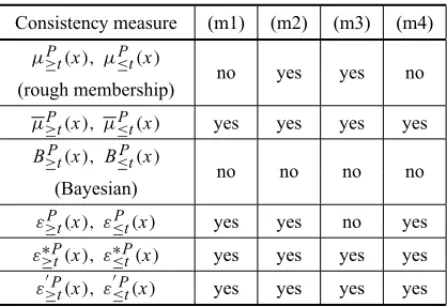
To be concordant with the rough set philosophy, consistency measures should enjoy some mono-tonicity properties (see Table 1). A consistency measure is monotonic if it does not decrease (or does not increase) when:
(m1) the set of attributes is growing,
(m2) the set of objects is growing,
(m3) the union of ordered classes is growing,
(m4) ximproves its evaluation, so that it dominates more objects.
As to the consistency measuresε′≥Pt(x)andε′≤Pt(x)which enjoy all four monotonicity properties, they can be interpreted as estimates of conditional probability, respectively:
Pr(y∈D+P(x)|y∈ ¬Clt≥) , Pr(y∈D−P(x)|y∈ ¬Cl
≤
t ) .
They say how far the implications
y∈D+P(x)⇒y∈Clt≥, y∈ D−P(x)⇒y∈Cl
≤
t
Table 1– Monotonicity properties of consistency measures (Blaszczynski, Greco, Slowinski & Szelag, 2009).
Consistency measure (m1) (m2) (m3) (m4)
µ≥Pt(x), µ≤Pt(x)
no yes yes no
(rough membership)
µ≥Pt(x), µ≤Pt(x) yes yes yes yes B≥Pt(x), B≤Pt(x)
no no no no
(Bayesian)
ε≥Pt(x), ε≤Pt(x) yes yes no yes ε≥∗Pt(x), ε≤∗Pt(x) yes yes yes yes ε≥′Pt(x), ε≤′Pt(x) yes yes yes yes
For every P ⊆C, the objects being consistent in the sense of the dominance principle with all upward and downward unions of classes are calledP-correctly classified. For every P⊆C, the
quality of approximation of classification Clby the set of criteriaPis defined as the ratio between the number of P-correctly classified objects and the number of all the objects in the decision table. Since the objects which are P-correctly classified are those that do not belong to any P -boundary of unionsClt≥andCl≤t ,t =1, . . . ,n, the quality of approximation of classification
Clby set of criteria P, can be written as
γP(Cl) =
U− S
t∈{1,...,n}
BnP(Clt≥)
!
∪ S
t∈{1,...,n}
BnP(Clt≤)
!!
|U|
=
U− S
t∈{1,...,n}
BnP(Clt≥)
!!
|U|
γP(Cl)can be seen as a measure of the quality of knowledge that can be extracted from the decision table, where Pis the set of criteria andClis the considered classification.
Each minimal subsetP⊆C, such thatγP(Cl)=γC(Cl), is called areductofCland is denoted by R E DCl. Note that a decision table can have more than one reduct. The intersection of all reducts is called thecoreand is denoted byC O R ECl. Criteria fromC O R EClcannot be removed from the decision table without deteriorating the knowledge to be discovered. This means that in setCthere are three categories of criteria:
• indispensablecriteria included in the core,
• exchangeablecriteria included in some reducts but not in the core,
Note that reducts are minimal subsets of criteria conveying the relevant knowledge contained in the decision table. This knowledge is relevant for the explanation of patterns in a given decision table but not necessarily for prediction.
It has been shown in (Greco, Matarazzo & Slowinski, 2001d) that the quality of classification satisfies properties of set functions which are called fuzzy measures. For this reason, we can use the quality of classification for the calculation of indices which measure the relevance of particular attributes and/or criteria, in addition to the strength of interactions between them. The useful indices are: the value index and interaction indices of Shapley and Banzhaf; the interaction indices of Murofushi-Soneda and Roubens; and the M ¨obius representation. All these indices can help to assess the interaction between the considered criteria, and can help to choose the best reduct.
4.3 Stochastic dominance-based rough set approach
From a probabilistic point of view, the assignment of objectxi to “at least” classtcan be made with probability Pr(yi ≥ t|xi), whereyi is classification decision for xi,t = 1, . . . ,n. This probability is supposed to satisfy the usual axioms of probability:
Pr(yi ≥1|xi)=1, Pr(yi ≤t|xi)=1−Pr(yi ≥t+1|xi), and Pr(yi ≥t|xi)≤ Pr(yi ≥t′|xi) for t≥t′. These probabilities are unknown but can be estimated from data.
For each classt=2, . . . ,n, we have a binary problem of estimating the conditional probabilities
Pr(yi ≥ t|xi)= 1, Pr(yi < t|xi). It can be solved byisotonic regression(Kotlowski, Dem-bczynski, Greco & Slowinski, 2008). Letyi t =1 ifyi ≥t, otherwiseyi t =0. Let also pi t be the estimate of the probability Pr(yi ≥ t|xi). Then, choose estimates p∗i t which minimize the squared distance to the class assignmentyi t, subject to the monotonicity constraints:
Minimize
|U| P
i=1
(yi t−pi t)2
subject to xi xj → pi t ≥ pj t for allxi,xj ∈U wherexi xj means thatxidominatesxj.
Then, stochasticα-lower approximations for classes “at leastt” and “at mostt−1” can be defined as:
Pα(Clt≥) =
xi ∈U : Pr(yi ≥t|xi} ≥α ,
Pα(Clt≤−1) =
xi ∈U : Pr(yi <t|xi} ≥α .
Replacing the unknown probabilitiesPr(yi ≥ t|xi), Pr(yi < t|xi), by their estimates pi t∗ ob-tained from isotonic regression, we get:
Pα(Clt≥) =
xi ∈U: p∗i t ≥α ,