T. G. Ritto
[email protected] Department of Mechanical Engineering Federal University of Rio de Janeiro (UFRJ), RJ, BrazilF. S. Buezas
[email protected] Departamento de F´ısica Universidad Nacional del Sur, CONICET ArgentinaRubens Sampaio
[email protected] Department of Mechanical Engineering PUC-Rio, RJ, BrazilProper Orthogonal Decomposition for
Model Reduction of a Vibroimpact
System
The application that inspires this work is the percussion drilling. This problem has impacts and presents uncertainties. In this first analysis the focus is on the construction of an efficient reduced-order model to deal with the nonlinear dynamics due to the impacts. It is important to have an efficient reduced-order model to perform the stochastic analysis. The simplified full model is constructed using the finite element method, and three different bases are used to construct the reduced-order models: LIN-basis (composed by the normal modes of the associated linear problems), PODdir-basis (obtained through proper
orthogonal decomposition - direct method) and PODsnap-basis (obtained through proper
orthogonal decomposition - snapshot method). The shapes of the elements of LIN-basis, PODdir-basis, and PODsnap-basis are compared. One important conclusion is that the
information necessary to represent the details of a vibroimpact dynamics, measured by the proper orthogonal values, is more than the usual 99% recommended.
Keywords: model reduction, proper orthogonal decomposition (POD), Karhunen-Lo`eve expansion, vibroimpact system, nonlinear dynamics
Introduction
The application that inspires this work is the percussion drilling (Batako et al. (2003); Wiercigrocha et al. (2001); Aguiar (2010)). The hard and expensive conditions which is subjected machinery performing drilling justify its modeling and study. These are systems with impacts and uncertainties (within the parameters of the system, for example).
The focus of the present analysis is on the construction of an effective reduced-order model for a vibroimpact system, and a simple model of a bar impacting an obstacle is used for this purpose. It is important to have an efficient reduced-order model for a future stochastic analysis. There are several approaches concerning reduced-order modeling; the present work is concerned with model reduction through the modal basis and through the proper orthogonal decomposition (POD). The LIN-basis (basis composed by the normal modes of the system) is the best basis for a linear dynamical system (Trindade et al. (2005)), but the basis generated by POD has the capacity to describe the phenomenon of interest (linear or nonlinear dynamics, for example) in a reduced dimension that is able to capture most of the phenomenon (Holmes et al. (1996)). It can be used as a tool for signal analysis, imaging processing, and other applications. In Mechanical Engineering its first applications were in turbulence (Lumley (1970)). POD-basis is the best basis of projection for the Galerkin method in the sense that it minimizes the average squared distance between the original data and its reduced linear representation. The group of PUC-Rio has been working on this subject for a while (Sampaio and Wolter (2001); Wolter (2001); Trindade and Sampaio (2001); Wolter et al. (2002)). Recently three works have been published by Bellizzi and Sampaio (2006, 2009a,b). Vibroimpact systems are relevant (Ibraim (2009)), particulary for the modeling of percussion drilling (Batako et al. (2003); Wiercigrocha et al. (2001)). The objectives of this paper are: 1) to present and compare, in a didactic and detailed form, these reduction techniques for a simple vibroimpact system, 2) to quantify which strategy is better to be used in the future for the stochastic analysis, and 3) to investigate whether the use of 99% (or 99.9%) of the information in the reduced-order model (suggested by Sirovich
Paper received 21 July 2010. Paper accepted 9 May 2011.
Technical Editor: Fernando Rochinha
(1987); Ma et al. (2008); Azeez and Vakakis (2001); Trindade et al. (2005)) is sufficient to represent the details of the impact.
The article is organized in the following manner. First, the formulation of the problem is presented, then the dynamical system is discretized by means of the finite element method (FEM). The model is reduced using: LIN-basis (direct method and snapshot method). The numerical results are later discussed, where the efficiency of the bases used in the Galerkin method is analyzed. Finally, the concluding remarks are made. Two appendix give more information about the numerical simulations used for the construction of the POD-basis.
Nomenclature
A = beam cross sectional area ai = i-th expansion coefficients c = damping coefficient d = beam diameter e(%) = percent error
E = elasticity modulus of the material E[·] = expected value
f = excitation force
gap = distance between bar–obstacle ki = obstacle stiffness
L = length of the beam M = number of time instants
N = Newton (unit of force), number of test functions, or number of spatial points, depending on the context
Pimp = impact force
PL = force at the end of the beam R(x,x′) = autocorrelation
u = longitudinal displacement field of the bar V = admissible space
f = force vector
u = response vector [C] = damping matrix [K] = stiffness matrix [M] = mass matrix
Greek Symbols
ωi = i-th natural frequency φ = test function
ρ = volumetric density of the material
Mathematical Model
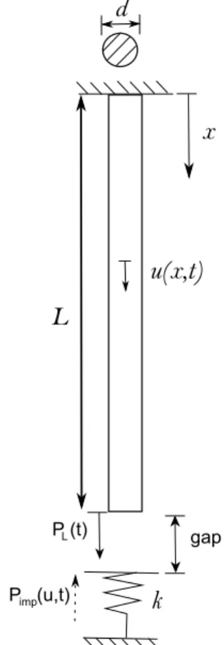
The simplified model considered in the present analysis is sketched in Fig. 1.
Figure 1. Scheme of a bar impacting an obstacle.
Letube the longitudinal displacement of the bar,Ethe elasticity modulus of the material,ρthe volumetric density of the material, and Athe beam cross-sectional area. The boundary conditions are given by
u(x=0) =0 (essential)
EA∂u
∂x(x=L) =0 (natural),
(1)
wherex=0 is the fixed end andx=Lis the free end. The initial conditions are the following:
u(t=0) =u0 ∂ u
∂t(t=0) =v0. (2) We assume that A, E and ρ are constants in x. A dissipation term (viscous damping) and an excitation force are added to the formulation. The equation of motion for this model is given by
−EA∂ 2u(x,t)
∂x2 +c ∂u(x,t)
∂t +ρA∂ 2u(x,t)
∂t2 = f(x,t,u), (3)
wherecis the damping coefficient and fis the excitation force:
f(x,t,u) =PL(x,t) +Pimp(x,t,u), (4)
in whichPLis an imposed sinusoidal force andPimpis the percussive force (detailed in the sequence). The bar is excited on its free extremity and the movement of the bar is limited by an obstacle. The impact is modeled by an elastic force, proportional to the obstacle stiffness; and it introduces a nonlinearity into the system. Between impacts the system is linear and the impact redistributes the energy in the system among the different modes. The forcesPLandPimpare written as
PL(x,t) =Pfsin(ωft)δ(x−xL), (5)
Pimp(x,t,u) =Pc(u,t)δ(x−xL), (6)
in which
Pc(u,t) =−γ[ki(u(L,t)−gap)]
γ=0 i f u(L,t)<gap γ=1 i f u(L,t)>gap,
(7)
whereu(L,t)is the displacement atx=L,gapis the distance from the bar to the obstacle andkiis the obstacle stiffness. Observe that the
dependence ofPLonxLis showed by the subscriptL.
Finite Element Method
The element used in the finite element discretization is linear, and the discretized system is given by:
[M]¨u(t) + [C]˙u(t) + [K]u(t) =f(u(t),t), (8)
where[M]is the mass matrix,[K]is the stiffness matrix,[C]is the proportional damping matrix,uis the response of the system andfis the force vector that includes the excitation force and the force due to the impacts. FEM is widely used and it is very effective. Nevertheless, depending on the problem, one can deal with huge matrices. Besides that, a nonlinear analysis can be very time consuming. To diminish these problems, huge matrices and large simulation time, we reduce the model using appropriate bases of projection.
Reduced-Order Model
Matrices[M],[C]and[K]have dimensionm×m. Considering[Q] with dimensionm×n(n<m), composed by independent vectors, one introduces the change of variables:
u(t) = [Q]a(t). (9)
Then, Eq. (8) becomes:
Matrix [Q] is composed by m orthogonal vectors that generate a reduction subspace into which the dynamics will be projected. Projecting the dynamics on the subspace generated by the new basis:
[Q]T[M][Q]¨a(t) + [Q]T[C][Q]˙a(t) + [Q]T[K][Q]a(t) =
= [Q]Tf([Q]a(t),t),
(11)
which can be written as
[Mr]¨a(t) + [Cr]˙a(t) + [Kr]a(t) = [Q]Tf([Q]a(t),t), (12)
where the reduced matrices are[Mr] = [Q]T[M][Q],[Cr] = [Q]T[C][Q],
and[Kr] = [Q]T[K][Q]. Matrix[Mr]has dimensionn×n, thus, the size
of the matrices are reduced fromm×mton×n, wheren<m. One can expect to solve the time-integration problem much faster with the reduced-order model, although it is not assured (Ritto et al. (2011)).
Modal basis
The modal basis can be used as trial functions in the Galerkin method. If a linear system with proportional damping matrix is the one analyzed, then the basis generated by the normal modes are the optimum basis (Trindade et al. (2005)). When dealing with a nonlinear problem one faces a difficulty, because there is no such thing as normal modes. Of course, one can associate to a nonlinear model a linear one, and use the normal modes of the linear problem to construct the reduced-order model.
The normal modes and the natural frequencies can be found by solving the following characteristic value problem:
(−ω2i[M] + [K])φi=0, (13)
whereωiis thei-th natural frequency andφiis thei-th normal mode.
LIN-basis is the basis composed by these normal modes. For a bar fixed at one end and free at the other, they can also be calculated directly by the analytical expression (Blevins (1993)):
φi(xj) =sin
(2i−1)π 2L xj
, (14)
wherexjare the node points.
Proper Orthogonal Decomposition (POD)
POD can be used as trial functions in the Galerkin method and it is the optimum basis (in the least square sense, see Holmes et al. (1996)) to represent a dynamical problem. Hence, fixing the first Ncomponents of the basis, no other linear decomposition (withN components) will better represent the dynamics than POD. It should be noticed that not necessarily the time-integration will be solved faster using POD-basis (Ritto et al. (2011)).
The system response is modeled as a second-order stochastic process. There are two important assumptions: the process is stationary in time and ergodic (Holmes et al. (1996)).
POD-basis is sensitive to loads, which means that dynamical responses must be obtained, for instance, for different ranges of excitation (e.g., 100N<Pf <200N). In this case, POD-basis is
supposedly valid to represent systems which are excited in this force band.
As shown by Sampaio and Wolter (2001), there are two methods for constructing POD-basis: the direct method and the snapshot method.
Direct method
Letu(·,t)be a vector field inΩ⊂R3andt∈R, i.e.,u(x,y,z,t). Decomposinguin two parts: one invariant in timeE[u(·,t)]and another with zero meanv(·,t):
v(·,t) = u(·,t)
| {z } response
−E[u(·,t)]
| {z }
mean
, (15)
then, v(·,t) is a stochastic process with zero mean and, as a consequence, its correlation is equal to its autocorrelation (Papoulis (1991)). Ifvis real, then the spatial autocorrelation of two points is defined by:
R(x,x′) =E[v(x,t)v(x′,t)]. (16)
Using the ergodicity hypothesis, one may write:
R(x,x′) =1 τ
Zτ
0 v(x,t)v(x ′,t)dt,
(17)
where τ is the duration of the analysis. The eigenvalues (or proper orthogonal values, POVs) and the eigenfunctions (or proper orthogonal modes POMs) are computed solving the following eigenvalue problem:
Z
ΩR(x,x ′)ψ
k(x′)dx′=λkψk(x). (18)
Considering the discretized field:
u(xi,yj,zk,t), (19)
wherei,j,kassume values from 1 toNx,Ny,Nzrespectively. For each
instant of time there areNsample values,N=3×Nx×Ny×Nz. The
number 3 multiplying the expression is due to the three dimensional field (ux, uy and uz). In the present application there is only one
important dimension and one dimensional field, which arexandu, therefore,N=Nx.
The sample can be ordered: u(x1,·),u(x2,·), ...,u(xN,·). The
dynamical system displacement is experimentally measured or numerically calculated inNpoints andMinstants.
[U] = [u(x1,·) u(x2,·) ... u(xN,·)]=
u(x1,t1) u(x2,t1) ... u(xN,t1)
. . . .
. . . .
. . . .
u(x1,tM) u(x2,tM) ... u(xN,tM) . (20)
[V] = [U]− 1 M M
∑
i=1u(x1,ti) M
∑
i=1u(x2,ti) ... N
∑
i=1u(xN,ti)
. . . .
. . . .
. . . .
M
∑
i=1u(x1,ti) M
∑
i=1u(x2,ti) ... M
∑
i=1u(xN,ti) . (21)
The autocorrelation matrix is then constructed:
[R] = 1 M[V]
T[V], (22)
where the matrix [R] is symmetric by construction. The discretized eigenvalue problem is given by
[R]ψk=λkψk, (23)
which is the discretized version of Eq. (18). The eigenvectorsψk (POMs) generate the PODdir-basis, and the POVs are the eigenvalues (λk) of matrix[R]. Note that the dimension of matrix[R]depends only on the spatial discretization, but not on the time discretization. Therefore, the direct method is recommended when the spatial mesh is coarse and many instants are needed in the time-discretization to capture the system dynamics.
The algorithm to implement this kind of decomposition can be summarized by the following steps:
• Discretize the displacement field inM instants and inNspace points,[U]; see Eq. (20).
• Compute the zero-mean response,[V]; see Eq. (21).
• Construct the autocorrelation matrix[R](N×N); see Eq. (22).
• Solve the eigenvalue problem given by Eq. (23) to get the POMs and POVs.
Snapshot method
To compute the POMs using the direct method, it is necessary to solve an eigenvalue problem for matrix [R] (Eq. (22)). This matrix has dimensionN×N (related to the spatial discretization). The question that arises is if it is possible to compute the POMs solving an eigenvalue problem of another matrix ([D]) with dimension M×M(related to the time discretization). The answer is the snapshot method.
The goal is to compute ψ without using R directly. For this purpose, substituting Eq. (17) into Eq. (18):
Z
Ω 1 τ
Zτ
0 v(x,t)v(x ′,t)dtψ
k(x′)dx′=λkψk(x), (24)
which can be rewritten as:
1 τ
Zτ
0 v(x,t)
Z
Ωv(x ′,t)ψ
k(x′)dx′dt=λkψk(x). (25)
Therefore,ψkcan be written as:
ψk(x) =
Zτ
0
v(x,t) 1 τ λk
Z
Ωv(x ′,t)ψ
k(x′)dx′dt. (26)
Now let
Ak(t) = 1
τ λk
R
Ωv(x′,t)ψk(x′)dx′ −→ ψk(x) =R0τv(x,t)Ak(t)dt,
(27)
which means thatψk(x) is a linear combination ofv(x,t). For a
finite number of instantstm(m=1,2, ..,M), wheretm= (m−1)∆t,
a snapshot is defined as:
v(m)=v(·,tm). (28)
The value ofAk is still unknown. To calculate it, one should substitute Eq. (27) into Eq. (25):
1 τ
Rτ 0 v(x,t)
R
Ωv(x′,t)R0τv(x′,t′)Ak(t′)dt′dx′dt
=λkR0τv(x,t)Ak(t)dt.
(29)
which can be rewritten as:
Zτ
0
Zτ
0 Ak(t ′)1
τ
Z
Ωv(x
′,t)v(x′,t′)dx′dt′dt=λ k
Zτ
0 Ak(t)dt. (30) Now let
D(t,t′) =1 τ
Z
Ωv(x
′,t)v(x′,t′)dx′, (31)
thus,
Zτ
0
Zτ
0
Ak(t′)D(t,t′)dt′dt=λk
Zτ
0
Ak(t)dt. (32)
Discretizing the above equation, one has
[D]Ak=λkAk. (33)
Hence, the POMs (ψk) can be computed using Eqs. (32) and (27). Summarizing what has to be done for the construction of the POD-basis using the snapshot method: first, matrix[D]is computed using [V](see Eqs. (31) and (21)):
[D] = 1 M[V][V]
T. (34)
It has dimensionM×M, instead ofN×Nas matrix[R](see Eq. (22)). The eigenvalues of[D]are the POVs, but the POMs are computed using the following equation:
which is the discretized version of Eq. (27), where Ak are the eigenvectors of matrix[D]. The POMsψkare linear combinations of the snapshots, which are the lines of matrix[V].
Note that the dimension of matrix [D] depends only on the number of snapshots; it does not depend on the spatial discretization. Therefore, the snapshot method is recommended when the spatial mesh is fine and there are not many instants, as in rapidly decaying processes.
The algorithm to implement this kind of decomposition can be summarized by the following steps:
• Calculate matrix[D](dimensionM×M) using[V]; see Eqs. (21) and (34).
• Compute the eigenvalues (POVs) and the eigenvectors of matrix [D]; see Eq. (33).
• Calculate the POMs using the eigenvectors of [D](which are
Ak) and[V]; see Eq. (35).
Numerical Results
The system of ordinary differential equations is numerically integrated through the routineode45, which is based on Runge-Kutta (Butcher (2003)) method of fourth an fifth order. Theode45uses an adaptive time-step to compute the time response. The maximum error allowed was 10−6. A∆tequal to 10−5is used to visualize the result.
The computer used to run the simulations was a Pentium(R) (32-bits), 2 GB RAM and 3.2 GHz. Figure 1 represents the bar considered in the simulations. Table 1 shows the values of the parameters used for the simulations.
Table 1. Data used in the simulations. Length,L=1m
Diameter,d=100mm
Elasticity modulus,E=200GPa Density,ρ=7850kg/m3 Damping factor,c=10000Ns/m2 Obstacle stiffness,ki=1e11N/m
Distance between bar-obstacle,gap=0.1µm
Excitation force: Pfsin(ωft), Pf =5000N andωf =2π260
rd/s. The error analysis is made by using the following norm:
ku(t)k=
s
Z
Ω(u(x,t)) 2
dx+
Z
Ω
∂u(x,t)
∂x
2
dx.
The percent error is calculated by the formula:
e(%) = 100 t1−t0
Zt1
t0
ku(t)n−u(t)n−1k ku(t)nk
dt, (36)
whereunis the approximation of the response withnelements of the basis,un−1is the approximation of the response withn−1 elements, and[t0,t1]is the duration of the analysis.
General response
The system considered in this paper is simple, but the same procedure can be performed for more complicated situations as it was done in Trindade et al. (2005). One motivation to study a vibroimpact
system is its applications on drilling systems. In this section we show some general aspects of the dynamical response.
Figure 2 shows the dynamical response and the impact forces at x=L; the forces due to the impact are approximately 5000N(peak).
0 0.005 0.01 0.015 0.02
−3.5 −3 −2.5 −2 −1.5 −1 −0.5 0 0.5x 10
−6
Time (s)
u L
(t)
(a)
0 0.005 0.01 0.015 0.02 0 1000 2000 3000 4000 5000 6000 Time (s) P imp (N) (b) Figure 2. (a) Dynamical response atx=L(the dashed line shows the obstacle position) and (b) force due to impact atx=L.
Figure 3 shows the dynamical response close to the impact region for two different damping coefficients. Whenc=105Ns/m2one can see how the reflection waves alter the movement of the bar (steps), but whenc=106Ns/m2the structure is overdamped.
At this point, we have presented some general aspects of the vibroimpact dynamics. In the remainder of this section the properties of each of the methods proposed to construct the reduced-order model are compared.
FEM, LIN-basis, and POD comparison
The dynamical response was calculated and the error (Eq. (36)) was computed varying the number of elements of the basis. As a matter of organization, the details on how the POD-bases have been generated are found in Appendices A and B. It should be noted that the sample needed to construct a POD-basis does not need to be so large. For the problem analyzed, an autocorrelation matrix of dimension 1000 x 1000 was good enough (see the Appendices A and B).
0.0155 0.016 0.0165 0.017 0
5 10 15
x 10−8
Time (s)
Displacement (m)
(a)
0.0155 0.016 0.0165 0.017 0.0175 0
5 10 15
x 10−8
Time (s)
Displacement (m)
(b) Figure 3. Impact detail of the response of the system forc=105(a) and106
Ns/m2(b). The dashed line shows the impact location.
0 50 100 150
0 2 4 6 8 10 12 14
Number of elements of the basis
Percent error
FE LIN−basis POD−basis
Figure 4. Convergence comparison for three different reduction bases: FE, LIN-basis, and POD-basis.
In Fig. 5 one can notice that the two convergences (direct and snapshot) look very alike. For an error of 1% it is necessary 50 POMs from both POD-direct, and POD-snapshots.
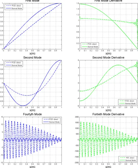
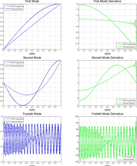
A comparison between POMs and normal modes is done in Figs. 6 (PODdir) and 7 (PODsnap). Both POMs and normal modes are zero atx=0 and derivatives equal zero atx=L. The modes were
10 20 30 40 50
0 1 2 3 4 5 6 7
Number of empirical modes
percent error
POD−direct POD−snapshot
Figure 5. Convergence comparison for POD-direct and POD-snapshots.
normalized to have value one atx=L. POMs are different from normal modes, but their derivatives are even more different, which is an important fact since the mode derivatives are used to construct matrix[K].
The shapes of the normal modes are given by the sinus function. On the other hand, the shape of the POMs are given by the response of the nonlinear dynamics. This is the reason why they can capture the nonlinearities of the dynamics. Note that the fortieth POM represents a movement where there is more restriction to move close to the impact region.
The two first POMs obtained by direct (Fig. 6) and POD-snapshots (Fig. 7) are very close to each other. They are the modes that have the larger contribution to the dynamics (they are related to the two highest POVs). But the other POMs are different, as shows the fortieth POM. The POMs depend on the sample used to construct the basis. Table 2 shows the first POV (Proper Orthogonal Values) from both POD-direct and POD-snapshots.
Table 2. Proper orthogonal values (POVs).
POV Direct method Snapshot method
λ1 0.998396 0.998498
λ2 0.001472 0.001385
λ3 0.000054 0.000056
λ4 0.000037 0.000032
λ5 0.000015 0.000014
The sum of the first five POVs, for the direct method as for the snapshot method, is 0.99998, what represents a high level of information of the model. This means that 99.998% of the dynamics are in the five first PODs.
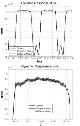
Figure 8 shows the dynamical response atx=L approximated with five POMs. One can see that the overall dynamics is well represented. But in the impact region there is a big difference, especially in the derivatives ofu. Please note that the first derivative is also taken into account in the error.
Figure 6. Normal modes x POM-direct.
be considered to represent the problem; the first POV has more than 99.9% of the energy and the solution presents a considerable difference in the impact detail. This means that in the impact region one do no better, inaccuracies are germane to impact problems. If the excitation frequency was lower or higher, one should expect the same kind of results. In this case, the simulations used to construct POD-basis (see Appendices A and B) should take into account the new excitation frequency. If the impact stiffness decreases or if the damping of the system increases, one should expect to represent the system with less elements of the basis (hence, less information). Taken the limit where the system is overdamped or if the impact stiffness is zero, it is clear that the dynamical response of the system gets much simpler.
Concluding Remarks
Three reduction strategies (using LIN-basis, PODdir-basis and PODsnap-basis) were presented in detail and compared, for a simple vibroimpact system. The inspiration for the construction of a reduced-order model is the stochastic analysis of a percussion drilling system. The main contributions of this paper are: 1) the comparison and analysis of the reduction techniques for a vibroimpact system,
2) the conclusion that the POD-basis is the best reduction basis for the problem (which is not a straightforward conclusion, see Sampaio and Soize (2007)) and should be used in the future for the stochastic analysis, and 3) the conclusion that, contrary to previous recommendation, 99.9% of the information (POV) might not be good enough to represent the impact details of the dynamical response of a vibroimpact system, as showed in Fig. 8; though it may be good enough to reconstruct the overall dynamics.
For a future stochastic analysis, one should note that the basis constructed through POD is specific for the system analyzed with specified parameters, boundary conditions and exciting forces. This means that if a parameter changes significantly, the POD-basis may not be efficient to represent the system with this new parameter. To avoid this problem and to construct a more general POD-basis, many simulations are done with different values for the parameters (see Appendices A and B) in a way that this basis should be good to represent different situations. This is especially important for a stochastic analysis, where some parameters are modeled using random variables. However, this needs further investigation.
Figure 7. Normal modes x POM-snapshots.
approximation of the response using LIN-basis (80 elements) or POD-basis (40 elements), is due to the disconnection between the interpolation functions of FEM with the dynamics in analysis. POD is able to capture the nonlinearities of the dynamical response and, therefore, it can represent the problem in a reduced manner.
Acknowledgements
The authors gratefully acknowledge the support of Conselho Nacional de Desenvolvimento Cient´ıfico e Tecnol´ogico (CNPQ), Fundac¸˜ao de Amparo `a Pesquisa do Estado do Rio de Janeiro (FAPERJ), andConsejo Nacional de Investigaciones Cient´ıficas y T´ecnicasCAPES-MINCyT.
Appendix A - Numerical Simulations for the Construction of POD-Basis - Direct Method
The POD-basis is calculated from several dynamical responses. Ten simulations (t=0.02s) were performed with different excitation forces, varying from 4000 N to 6000 N. Two points should be noted:
1. POD-basis computed for a set of parameters may not be good to represent the system with another set of parameters, as will be showed
later.
2. If data is increased, the sample is better and the POD-basis is more reliable. But to compute quickly the basis, one searches to get strictly the necessary information. In the case of POD-direct, the fewer spatial points as possible and in the case of POD-snapshots, the fewer instants (snapshots) as possible. This is due to how the bases are constructed.
Since only the last 0.01 s was considered in the computations and ∆t=10−5, matrix[U], Eq. (20), has 10000 lines. To investigate the generation of the basis through POD-direct method, first one considers 1000 spatial points (see the convergence in Fig. 5).
In real applications it is not feasible to measure the displacement in 1000 points. Another POD-basis was generated considering 100 spatial points, see Fig. 9.
(a)
(b) Figure 8. (a) Approximation of the response with five POMs and (b) detail of the impact.
Figure 9. POD-basis convergence (using100spatial points).
Appendix B - Numerical Simulations for the Construction of POD-Basis - Snapshot Method
To investigate the generation of the basis through POD-snapshots method, first one considers 3000 snapshots and 1000 spatial points (see the convergence in Fig. 5). Then, one tries to reduce the number of snapshots and still get a good basis; this strategy is different from POD-direct where one wants to get less spatial points.
Figure 11 shows the convergence analysis for POD-basis
Figure 10. POD-basis convergence (using10spatial points).
Figure 11. POD-basis convergence (1000snapshots).
generated with 1000 snapshots (0.01 s, ∆t = 10−5s). This convergence is almost as good as the one using 3000. One needs now 50 POMs for a precision of 2%.
To reduce the snapshots, but keeping the coherent structure, only one cycle of the dynamical response will be considered. Figure 12 shows the points in time where the snapshots are taken; only the snapshots atx=L, but the snapshots are taken for all of the 1000 spatial points.
Figure 13 shows the convergence analysis for POD-basis generated considering one cycle of the response and 400 snapshots. This convergence is not as good as the one using 3000, since one needs 60 POMs, instead of the 50 needed before to represent the problem. Finally, Fig. 14 shows the convergence analysis for POD-basis generated considering one cycle of the response and 40 snapshots; now the precision is not so good.
References
Aguiar, R.R., 2010, “Experimental investigation and numerical analysis of the vibro-impact phenomenon”, D.sc. thesis, Department of Mechanical Engineering, PUC-Rio, Brazil.
Azeez, M.F.A. and Vakakis, A.F., 2001, “Proper orthogonal decomposition (pod) of a class of vibroimpact oscillations”, Journal of
Sound and Vibration, Vol. 240, No. 5, pp. 859-889.
Batako, A.D., Babitsky, V.I., Halliwell, N.A., 2003. “A self-excited system for percurssive-rotary drilling”, Journal of Sound and Vibration, Vol. 259, No. 1-2, pp. 97-118.
Figure 12. Instants where the snapshots are taken (400snapshots,200snapshots,80snapshots and40snapshots).
Figure 13. POD-basis convergence (400snapshots).
systems obtained from Karhunen-Lo`eve expansion”, Journal of Sound and Vibration, Vol. 297, No. 3-5, pp. 774-793.
Bellizzi, S., Sampaio, R., 2009a, “Karhunen-Lo`eve modes obtained from displacement and velocity fields: Assessments and comparisons”,Mechanical
System and Signal Processing, Vol. 325, No. 3, pp. 491-498.
Bellizzi, S., Sampaio, R., 2009b, “Smooth Karhunen-Lo`eve decomposition to analyze randomly vibrating systems”, Journal of
Sound and Vibration, Vol. 23, No. 4, pp. 1218-1222.
Blevins, R., 1993, “Formulas for Natural Frequency and Mode Shape”, Krieger Publishing Company, USA.
Butcher, J.C., 2003, “Numerical methods for ordinary differential equations”, John Wiley & Sons, USA.
Holmes, P., Lumley, J., Berkooz, G., 1996, “Turbulence, coherent structures, dynamical systems and symmetry”, Cambridge University Press, UK.
Ibraim, R., 2009, “Vibro-Impact Dynamics”, Springer-Verlag Berlin Heidelberg.
Lumley, J.L., 1970, “Stochastic tools in turbulence”, Academic Press, USA.
Figure 14. POD-basis convergence (40snapshots).
Ma, X., Vakakis, A.F., Bergman, L.A., 2008. “Karhunen-Lo`eve analysis and order reduction of the transient dynamics of linear coupled oscillators with strongly nonlinear end attachments”,Journal of Sound and Vibration, Vol. 309, No. 3-5, pp. 568-587.
Papoulis, A., 1991, “Probability, Random Variables, and Stochastic Processes”, McGraw-Hill, USA.
Ritto, T.G., Buezas, F.S., Sampaio, R., 2011, “A new measure of efficiency for model reduction: Application to a vibroimpact system”,Journal of Sound
and Vibration, Vol. 330, No. 9, pp. 1977-1984.
Sampaio, R., Soize, C., 2007, “Remarks on the efficiency of POD for model reduction in non-linear dynamics of continuous elastic systems”,
International Journal for Numerical Methods in Engineering, Vol. 72, No. 1,
pp. 22-45.
Sampaio, R., Wolter, C., 2001, “Bases de Karhunen-Lo`eve: Aplicac¸˜oes `a mecˆanica dos s´olidos”, APLICON, S˜ao Carlos, SP, Brazil.
Sirovich, L., 1987, “Turbulence and the dynamics of coherent structures part I: coherent structures”,Quarterly of Applied Mathematics, Vo. 45, No. 3, pp. 561-571.
Decomposition of coupled axial/bending vibrations of beams subjected to impact”,Journal of Sound and Vibration, Vol. 279, pp. 1015-1036.
Wiercigrocha, M., Wojewodab, J., Krivtsovc, A.M., 2001, “Dynamics of ultrasonic percussive drilling of hard rocks”,Journal of Sound and Vibration, Vol. 280, pp. 739-757.
Wolter, C., 2001, “Uma introduc¸˜ao `a reduc¸˜ao de modelos atrav´es da expans˜ao de Karhunen-Lo`eve”, MSc. dissertation, Department of Mechanical Engineering, PUC-Rio, Brazil.
Wolter, C., Trindade, M.A., Sampaio, R., 2001, “Obtaining mode shapes through the Karhunen-Lo`eve expansion for distributed-parameter linear system”,Shock and Vibration, Vol. 9, pp. 177-192.
Wolter, C., Trindade, M.A., Sampaio, R., 2002, “Reduced-order model for impacting beam using the Karhunen-L`oeve expansion”,Tendˆencias em