www.nat-hazards-earth-syst-sci.net/10/2009/2010/ doi:10.5194/nhess-10-2009-2010
© Author(s) 2010. CC Attribution 3.0 License.
and Earth
System Sciences
Probabilistic projections for 21st century European climate
G. R. Harris, M. Collins, D. M. H. Sexton, J. M. Murphy, and B. B. B. Booth
Met Office, Hadley Centre, Exeter EX1 3PB, UK
Received: 10 December 2009 – Revised: 7 July 2010 – Accepted: 5 September 2010 – Published: 29 September 2010
Abstract.We present joint probability distribution functions of future seasonal-mean changes in surface air temperature and precipitation for the European region for the SRES A1B emissions scenario. The probabilistic projections quantify uncertainties in the leading physical, chemical and biological feedbacks and combine information from perturbed physics ensembles, multi-model ensembles and observations.
1 Introduction
Global Climate Models (GCMs) can provide detailed predic-tions of future climate change, solving the physical, chemical and biological equations which describe the climate system. However, GCMs are not perfect representations of the real world. The size of the grid is limited by the availability of computer resources and the representation of sub-grid scale processes is approximate, and limited by our ability to fully understand and measure climate processes. The consequence of this is that predictions of the future made using climate models are uncertain.
Model development and improvement to reduce this un-certainty is one of the principal activities of climate change research. Nevertheless, climate change is occurring now, and it is incumbent upon climate modellers to provide the best in-formation as soon as they can, to allow society to plan for the impacts of climate change. Our goal therefore is to quantify the uncertainty in predictions of future climate change, and using observational constraints to assess the relative likeli-hood for different model projections, arrive at climate pre-dictions that can be presented in the form of probability dis-tribution functions (PDFs). PDFs are essential to the impacts community for risk assessment of the impacts associated
Correspondence to:G. R. Harris
with climate change (Pittock et al., 2001). In this study, we concentrate on projections of surface air temperature and pre-cipitation for the European region, work undertaken as part of the ENSEMBLES project (Hewitt and Griggs, 2004; van der Linden and Mitchell, 2009). Projections sampled from these joint PDFs are available from: http://ensembles-eu. metoffice.com/secure/RT6 data 230609/data for RT6.html
It should be emphasised that the PDFs measure our uncer-tainty in the future climate based on our current understand-ing of the climate system and our current ability to model and observe it. They do not represent the frequency of oc-currence of future events, but rather the weight of evidence supporting different possible outcomes for a one-off future event. Hence they cannot be verified over repeated trials, in the same way that probabilistic weather or seasonal forecasts can be.
Section 2 introduces some of the issues in producing prob-abilistic climate projections, and outlines the approach we have developed to make the problem tractable. Section 3 pro-vides more details on the methodology. Section 4 describes probabilistic projections of temperature and precipitation for the European region, with illustrative examples. Some of the issues in the use and interpretation of the PDFs are discussed in Sect. 5, while in the concluding remarks in Sect. 6 we de-scribe how probabilistic projections could evolve in the fu-ture.
2 Probabilistic prediction of climate change
the existing (Murphy et al., 2007, 2009) and forthcoming publications for a more complete description of the method and its implementation. In contrast to the UKCP09 predic-tions, no regional downscaling is performed, although in all other respects the techniques used are identical. The pro-jections described here, and provided for the ENSEMBLES project (van der Linden and Mitchell, 2009) are therefore made at HadCM3 (Gordon et al., 2000) spatial scales of ap-proximately 300 km resolution.
A GCM numerically solves the equations of fluid motion that describe the atmosphere and ocean components of the climate system, albeit on spatial scales that generally fail to resolve all the cloud, thermodynamic, surface, cryosphere, biological and chemical processes that affect climate feed-backs and determine the response of the system to external forcing. These sub grid-scale processes are necessarily rep-resented by approximate bulk formulae, controlled by input parameters whose values are not precisely determined since they do not represent things we can measure directly. Dur-ing model development, the set of model input parameters that give the best simulation of current climate is sought, although due to the high number of parameters, there is as yet no way of being certain that the “best” set of parameters has indeed been used. Within the Bayesian framework the spread in response resulting from this modelling uncertainty is systematically quantified, and used to make probabilistic predictions.
In principle, given sufficient computing resources, appli-cation of the Bayesian methodology to the climate predic-tion problem should be relatively straightforward. Ideally, one would run a very large set of transient simulations of a GCM with interactive carbon-cycle fully coupled to a dy-namic ocean model, simultaneously perturbing all uncertain input parameters (including forcing), in order to fully sample uncertainties in the key climate feedback processes that in-fluence the climate response. The resulting ensemble of pos-sible model projections (the modelled “prior“ distribution), when weighted according to the ability of each model ver-sion to simulate global patterns of observed mean climate and recent historical trends, gives the “posterior” PDFs for future climate change. Recognizing that structurally differ-ent climate models possess potdiffer-entially differdiffer-ent systematic errors, one would seek to create similar “perturbed physics ensembles” (PPE) (Murphy et al., 2004) for as large a set of independent climate models as possible, to fully explore the range of possible climate response.
The ideal scenario outlined above is not possible given cur-rent computing resources, so to make the problem computa-tionally tractable, additional steps are required that introduce complexity to the probabilistic prediction methodology, and additional uncertainty to the projections. Firstly, we note that transient simulations with a dynamic ocean model re-quire long initial spin-ups to achieve quasi-equilibrium of the ocean and prevent drift of the model base climate. As these spin-ups are computationally very demanding, we choose
instead to explore the spread in equilibrium response ob-tained for a doubling of CO2concentration, with
perturba-tions applied to parameters of the atmospheric component only and coupling to a simple mixed-layer (“slab”) ocean model (Williams et al., 2001). Slab-ocean GCM simula-tions are less computationally demanding and faster to run, allowing much larger ensemble sizes that more fully explore the climate response. For the ENSEMBLES predictions, we have created an ensemble of 280 1×CO2and 2×CO2
atmo-sphere slab-ocean simulations. Even this relatively large en-semble is still too small to provide robust predictions for the distribution of response, due to the large number of uncertain input parameters. We therefore use the slab ensemble simula-tions to construct an “emulator” (Rougier et al., 2009), a sta-tistical representation of the GCM calculated using function-fits to the ensemble output. The model response (and asso-ciated error) for untried parameter combinations can be es-timated very rapidly using the emulator, so the response for large samples of the uncertain parameters can be used, allow-ing robust prediction of the equilibrium PDFs.
Impact modellers however wish to assess the risks of the effects of transient climate change, rather than those associ-ated with the equilibrium response. A time-scaling technique has therefore been implemented, which allows the transient regional response to be inferred from normalized equilibrium patterns of change (Harris et al., 2006). The local response in some surface climate variable of interest (e.g., surface temperature, precipitation) is assumed to be proportional to global mean surface temperature change1Tglb(t ), which is
rapidly obtained using a Simple Climate Model (SCM). The ability to vary climate forcing in the SCM also allows us to efficiently sample carbon cycle uncertainties and aerosol forcing uncertainty by tuning these components of the SCM to the response of transient GCM simulations.
Furthermore, it is not yet practicable to envisage the cre-ation of perturbed physics ensembles for more than one structurally independent model. Recognizing that predic-tions could still suffer from deficiencies arising from struc-tural errors in the model which cannot be resolved by varying its uncertain parameters (Rougier, 2007), we have developed a technique to include information from other GCMs of es-timates of the additional uncertainties associated with struc-tural errors. This approach adjusts the projections to account for potential biases arising from structural assumptions in HadSM3, and by combining results from perturbed physics and multi-model ensembles, avoids exclusive reliance on re-sults from a single model. Further details of this step, and time-scaling, are given in the next section.
3 Elements of the methodology
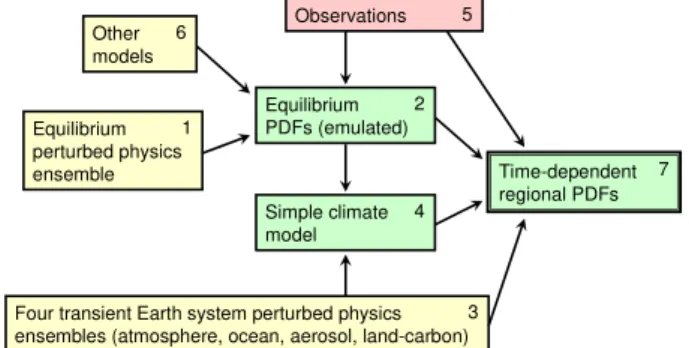
with each labelled step corresponding to the equivalent box in the flowchart in Fig. 1.
Box 1: Equilibrium perturbed physics ensemble
A relatively large ensemble of 280 1×CO2and 2×CO2
sim-ulations with the Hadley Centre HadSM3 model coupled to a simple slab ocean (Williams et al., 2001) has been pro-duced. In each model version, 31 uncertain parameters in the atmosphere and sea-ice components are varied (Murphy et al., 2004; Webb et al., 2006; Collins et al., 2010).
Box 2: Equilibrium PDFs (emulated)
The 280 member ensemble does not fully sample the re-sponse of the model to variations in the uncertain parame-ters, since the parameter space is so large. We therefore con-struct an emulator (Rougier et al., 2009) for the equilibrium response of HadSM3, trained on the 280 simulations. The emulator can predict the model response and associated error for any combination of parameter values, and is fast to use. Using the emulator, we can then robustly estimate the model response, sampling a large number of times the uncertain parameters, using expert judgement as to how they are dis-tributed (Murphy et al., 2004). A sample size of one million is used in this study. Each sampled projection is weighted by its likelihood given observed data (Box 5), and combin-ing the projections gives the posterior PDF for equilibrium response.
Box 3: Four transient Earth system perturbed physics ensembles
We have produced four smaller ensembles, each with 16 members, using the fully-coupled HadCM3 version of the model, in which the atmosphere is coupled to a dynamic ocean model (Gordon et al., 2000). An interactive sulphate aerosol component is always included. The ensemble mem-bers are driven by historical forcing, followed by the A1B SRES future forcing scenario (Naki´cenovi´c and Swart, 2000) to the end of the 21st century. In each of the ensembles, per-turbations are applied separately to: (i) the atmosphere and sea-ice parameters, (ii) ocean model parameters, (iii) param-eters in the sulphur-cycle component, and (iv) paramparam-eters in the land carbon cycle (e.g., Collins et al., 2006, 2007, 2010). Ensembles (ii) to (iv) use the standard (unperturbed) atmo-sphere parameter settings only. Land and ocean carbon cycle components were only included in the case of ensemble (iv). Box 4: Simple climate model
Since transient regional PDFs are required, we implement a time-scaling approach (Harris et al., 2006), which maps equi-librium changes in climate variables to transient changes un-der specified emissions scenarios. For a given set of model input parameters the normalised response is sampled from
Simple climate model
Time-dependent regional PDFs Equilibrium
perturbed physics ensemble
Four transient Earth system perturbed physics ensembles (atmosphere, ocean, aerosol, land-carbon)
Equilibrium PDFs (emulated) Other
models
Observations
1
2
4 5 6
7
3
Fig. 1.Flowchart showing the links between the seven components of the methodology described in more detail in Sect. 3 for the pro-duction of probabilistic predictions of future climate change. Boxes in red denote observational data, boxes in yellow represent ensem-bles of GCM simulations, and boxes in green represent statistical and other techniques required to convert the simulations into prob-abilistic predictions.
the emulation of the equilibrium response, and scaled by
1Tglb(t ) calculated from a SCM parameterised by global
climate feedbacks estimated from the equilibrium emula-tion. The radiative forcings (including aerosol forcing) used to drive the SCM are diagnosed from the HadCM3 simula-tions (Box 3). Time-scaling is validated by comparison with equivalent transient HadCM3 responses, and the errors as-sociated with this step are included in the scaled projections as an additional variance. Some of this scaling error is in-ternal variability in the GCM response that cannot be pre-dicted by a scaling of the mean response, and the rest is lack of fit associated with the scaling technique. The responses of perturbed climate-carbon simulations with HadCM3, and the C4MIP ensemble of coupled climate–carbon cycle sim-ulations (Friedlingstein et al., 2006) are used to tune land carbon cycle parameters in the SCM. Likewise the response of models in the CMIP3 archive (Meehl et al., 2007) and the HadCM3 ocean perturbed physics ensemble contribute to tuning of SCM parameters that control ocean heat uptake. By sampling the land carbon cycle and ocean parameterisa-tions in the SCM, we can efficiently sample uncertainties in the main global-scale feedbacks. Local climate-carbon feed-backs are therefore not modelled here, although for the Eu-ropean region they are less important than in regions such as the Amazon, where forest dieback and modification of local climate have been obtained (Cox et al., 2000).
Box 5: Observations
radiation at the top of the atmosphere, shortwave and long-wave cloud radiative forcing, total cloud amount, surface fluxes of sensible and latent heat, and latitude-height distri-butions of zonally averaged atmospheric relative humidity. The emulated equilibrium responses for the 48 observed cli-mate fields (12 variables for 4 seasons) are used in the likeli-hood expression to estimate relative weights associated with the different parameter combinations. Our expression for likelihood, Eq. (3.9) in Murphy et al. (2007), results from a Bayes linear analysis (Goldstein and Wooff, 2007) where uncertain quantities are represented in terms of means and a covariance matrix, thus taking into account relationships between variables. Likelihood weights are calculated in a re-duced dimension space, with a single weight being assigned for each model variant for all predicted variables (Murphy et al., 2009). Discrepancy (Box 6 below) between struc-turally different GCMs implies an additional modelling un-certainty. This is included in the likelihood weighting as an additional variance, and helps prevent poorly modelled vari-ables from overly constraining the distribution. Weights are also readjusted according to the ability of the scaled tran-sient projections to reproduce historical trends in four large-scale temperature variables (Braganza et al., 2003), which together explain much of the variance in spatiotemporal re-sponse (Stott et al., 2006). The historical trends used are: (i) global mean temperature, (ii) the land-ocean temperature difference, (iii) the inter-hemispheric temperature difference, (iv) the north-south temperature gradient in Northern Hemi-sphere mid-latitudes. Uncertainty in the magnitude of past climate forcing is accounted for in this step through the SCM (Box 4).
Box 6: Other models
Projections performed with the HadSM3 version with the “best” possible set of input parameters will still possess residual error (often termed “discrepancy”, e.g., Rougier, 2007) compared to both the observed past climate, and un-observed future climate. This additional uncertainty should be included in the projections. Discrepancy is a prior input to the statistical framework used to provide the projections, and should be calculated (as far as possible) independently of the observations used to weight them. Here we assume that structural differences between independent model pro-jections in the CMIP3 archive (Meehl et al., 2007) provide reasonable a priori estimates of possible structural errors be-tween HadSM3 and the real world. To obtain these “best” model residual errors, we search across the HadSM3 pa-rameter space for the set of papa-rameters that maximises the likelihood of reproducing the emulated climate and response to CO2 doubling for each of the CMIP3 models. These
estimates are made using the equilibrium simulations only. The historical component of discrepancy increases the uncer-tainty associated with comparisons between simulated past climates and observations, and therefore affects the weights
applied to emulated projections from different parts of pa-rameter space. The future component of discrepancy can al-ter the projected values and increase the spread in the poste-rior PDFs.
Box 7: Time-dependent regional PDFs
Sampling of the equilibrium weighted posterior distributions (Box 2) is performed to simultaneously predict the nor-malised local equilibrium response, and associated global climate feedbacks, which are used to drive the SCM. The predicted global temperature response1Tglb(t )is combined
with the local response to give the scaled projection. Un-certainty in response resulting from incomplete knowledge of the feedbacks between climate and the land carbon cycle is included by tuning components of the SCM to 24 alter-native realisations obtained from more complex coupled cli-mate carbon-cycle GCM simulations (Box 4). Carbon cycle uncertainty is thus accounted for through the global mean temperature response alone. The final PDFs are obtained by combining large samples of projections, with adjustment of the weights according to skill in predicting historical trends (Box 5).
Our methodology also allows us to predict the relative contributions of different components of uncertainty to the overall spread of the final PDFs. These include contributions from natural variability, model parameter uncertainty, struc-tural uncertainty, time-scaling, and carbon cycle uncertainty. Parameter uncertainty, dominated by atmospheric process uncertainty, generally provides the largest contribution al-though the other components all contribute significantly. No one single source of uncertainty dominates the total uncer-tainty. Further discussion of the sources of uncertainty in the PDFs can be found in Annex 2 of Murphy et al. (2009).
4 Probability distribution functions for Europe
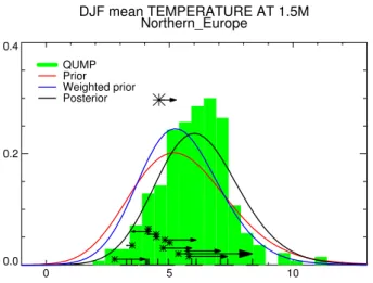
The method for obtaining the equilibrium PDFs is illustrated in Fig. 2, which shows equilibrium predictions for winter mean temperature for the large Northern European region (defined in Giorgi and Francisco, 2000) for a doubling of CO2. The output from the HadSM3 ensemble is used to train
DJF mean TEMPERATURE AT 1.5M Northern_Europe
0 5 10
0.0 0.2 0.4
QUMP Prior Weighted prior Posterior
Fig. 2. Equilibrium probability distributions functions for winter surface temperature change for the Giorgi-Francisco (2000) North-ern Europe region, following a doubling of CO2 concentrations. The green histogram (labelled QUMP) corresponds to the 280 equi-librium HadSM3 simulations used to construct a statistical emula-tor for this response. The red curve (labelled prior) is obtained from a large sample of emulated responses and is the prior distribution for this climate variable. The blue curve (labelled weighted prior) shows the effect of applying observational constraints to the prior distribution. The asterisks show the positions of our best emulated values of the 12 CMIP3 multi-model members and the arrows quan-tify the discrepancy between these best emulations and the actual multi-model responses. These discrepancies have a broadening ef-fect on the PDFs, and can shift the mean of the posterior distribution (black curve) relative to the weighted prior.
be shifted and the uncertainty increased by including the dis-crepancy term.
PDFs of transient seasonal-mean changes in surface air temperature and precipitation have been calculated using the techniques described above for the 2.5◦ latitude by 3.75◦
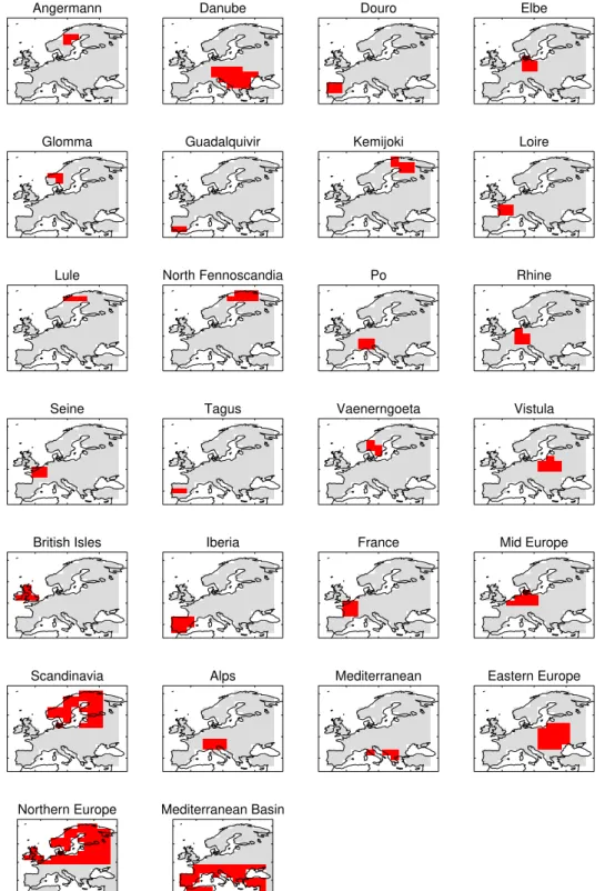
longitude HadCM3 grid boxes shown in Fig. 3, and for the aggregate regions shown in Fig. 4. The aggregate regions include 16 European river basins defined by ENSEMBLES partners, the 8 so-called “Rockel” regions of Europe defined for the PRUDENCE project (Christensen and Christensen, 2007), and the two Giorgi-Francisco regions covering Europe (Giorgi and Francisco, 2000). The PDFs represent changes in 20-year average climate for decadal steps starting from the period 2010–2029 and finishing at 2080–2099, expressed as anomalies computed with respect to a 1961–1990 climatol-ogy period. The distributions are conditional on the SRES A1B scenario of future emissions and represent a quantifica-tion of the uncertainty associated with major known physical, chemical and biological feedbacks, constrained by observa-tions of the climate system.
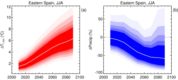
Figures 5, 6 and 7 show examples of the formats in which such PDFs can be presented; in this case the distributions are for the Eastern Spain grid box. The plumes in Fig. 5 show
the evolution of selected percentiles of the marginal proba-bility distributions for temperature and precipitation through the 21st century, in response to forcing under the A1B sce-nario. The term “marginal” here takes its usual meaning, e.g., the marginal temperature distribution is obtained by in-tegrating over all possible values of precipitation in the joint probability distribution. Figure 6 shows two possible repre-sentations of the joint distribution, in this case for the sum-mer response in Eastern Spain for the period 2080–2100. In Fig. 6a 10 000 sample points, drawn from the joint distribu-tion estimated using the methodology described in Sect. 3, are presented as a scatter plot. Each point can be treated as equally likely, with their density representing the underly-ing distribution. The PDFs produced for the ENSEMBLES project for European climate change, are supplied as sample data in this form. The use of 10 000 points is a compromise and may not give a particularly smooth picture of the PDF: many more sample points are required for this.
Analysis of the extreme tails of the distributions shows they can be sensitive to the statistical assumptions of the methodology (Murphy et al., 2009). This implies our con-fidence for points in the extreme tails is less than that for sample points in the central, more likely part of the distribu-tions. For this reason the sample data has been “Winsorised” at the 1st and 99th percentiles (see Sect. 5 below). The points coloured red in Fig. 6a correspond to the top and bottom 1% of the marginal distributions. Figure 6b presents the same data as Fig. 6a, but in the form of a contour plot. Use of a contour plot is recommended for presentation of results, since attention is drawn to the region of high probability, un-like the scatter plot presentation in Fig. 6a, where attention is more directed to the extreme, unlikely parts of the joint distribution. Correlation between the two variables is evi-dent for some grid boxes and seasons. For example, larger projected increases in summer temperature in Eastern Spain are associated with higher probabilities for reduced rainfall. Such relationships between variables reflect the response of the climate system to forcing explored by the ensembles of climate models used.
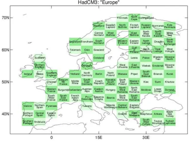
Fig. 3.The European region for which probabilistic projections have been provided as part of the ENSEMBLES project. All 106 HadCM3 land grid points as far east as Moscow and including Turkey have been selected and named. Southern Italy and the Mediterranean islands are not included since they are classed as ocean points in this model.
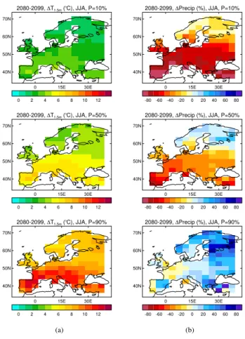
Finland. In this case, there is a positive correlation between increasing projected temperature and increased precipitation. Maps of 10, 50 and 90th percentiles for summer and win-ter surface air temperature and precipitation change by the end of the century are shown in Figs. 9 and 10. Median temperature changes vary substantially with location, and are largest in the Mediterranean region in summer and in north east Europe in winter. Note that the range of uncertainty, as measured here by the 10–90% range, is large for this time period: as much as 10 degrees Celsius in some locations. This is due to a combination of factors; parameter uncertainty in HadCM3, structural uncertainty from the CMIP3 ensem-ble, carbon cycle feedback uncertainty, internal variability and time-scaling uncertainty. No one source of uncertainty dominates (Murphy et al., 2009).
For the predictions of changes in precipitation, the canon-ical signals of summer Mediterranean drying and winter Northern Europe wetting are evident, but again the uncer-tainty range can be wide. For many grid boxes there are sig-nificant probabilities of both drier and wetter future climates and this may be important for impact studies. For some lo-cations in Southern Europe, the PDFs of projected
precipita-tion change show significant probabilities for large increases, when expressed as percentages. Care should be taken how-ever in interpreting these percentages changes when the present-day climatological precipitation (in the GCMs) is small.
5 Use of PDFs
Some aspects of the data describing the European predictions which arise predominantly because of practical considera-tions should be borne in mind when interpreting the data and using them to drive impact models.
Angermann Danube Douro Elbe
Glomma Guadalquivir Kemijoki Loire
Lule North Fennoscandia Po Rhine
Seine Tagus Vaenerngoeta Vistula
British Isles Iberia France Mid Europe
Scandinavia Alps Mediterranean Eastern Europe
Northern Europe Mediterranean Basin
Fig. 4.HadCM3 representation of the aggregate European regions for which probabilistic projections are supplied.
sampled population of 10 000. A simple test to check the robustness of sub-sampling would be to test the con-clusions of the impact study using different sub-sets of the sample data.
Eastern Spain, JJA
2000 2020 2040 2060 2080 2100
2 4 6 8 10 12
∆
T1.5m
(
o C)
(a)
Eastern Spain, JJA
2000 2020 2040 2060 2080 2100
-100 -50 0 50
∆
Precip (%)
(b)
Fig. 5. Evolution of the median (white curve) and the 50, 60, 70, 80 and 90% confidence intervals for: (a)20 year mean summer surface temperature change for the Eastern Spain grid point,(b)percentage change in 20 year mean summer precipitation for Eastern Spain.
Eastern Spain, JJA, 2080-2100
0 5 10 15
∆T1.5m (
oC)
-100 0 100 200 300 400
∆
Precip (%)
(a)
Eastern Spain, JJA, 2080-2100
0 5 10 15
∆T1.5m (
oC)
-100 -50 0 50 100
∆
Precip (%)
90% 80% 67% 33% % of Points Inside
(b)
Fig. 6. (a)Scatter plot of 10 000 sampled data points from the joint PDF of surface temperature change and percentage precipitation change for the summer season for Eastern Spain, for the period 2080–2099 relative to the 1961–1990 baseline period. Points that lie in the top and bottom 1% of the marginal distributions are shown in red.(b)Contours of the Winsorised sampled joint probability distribution function in (a).
of the distribution, compared with the tails. It is there-fore recommended that the 10th and 90th percentiles be used as a measure of the spread of the PDFs. Proba-bilities between 1 and 9%, and 91 and 99%, are to be used with caution as these are less robust. The level of robustness will vary according to variable, season and location (with temperature projections generally more robust than precipitation). Results concentrating on im-pacts of climate change which involve the more extreme percentiles of the distributions should be used with cau-tion.
PDF, Eastern Spain, JJA, 2080-2099, Temperature at 1.5m
0 5 10 15
∆T1.5m (
o C) 0.00
0.05 0.10 0.15 0.20
Winsorised sampled PDF Original PDF
CDF, Eastern Spain, JJA, 2080-2099, Temperature at 1.5m
0 5 10 15
∆T1.5m (
o C) 0.0
0.2 0.4 0.6 0.8 1.0
3.5 6.3 10.5
PDF, Eastern Spain, JJA, 2080-2099, Total Precipitation Rate
-50 0 50 100 150 200 250
∆Precip (%)
0.000 0.005 0.010 0.015
Winsorised sampled PDF Original PDF
CDF, Eastern Spain, JJA, 2080-2099, Total Precipitation Rate
-50 0 50 100 150 200 250
∆Precip (%)
0.0 0.2 0.4 0.6 0.8 1.0
-88 -57 32
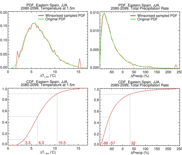
Fig. 7.PDFs and CDFs of surface temperature change and percentage precipitation change for the summer season for Eastern Spain for the period 2080–2099, relative to the 1961–1990 baseline period.(a)The marginal PDF and CDF for surface temperature change (red curves), corresponding to the Winsorised distribution in Fig. 6. The smooth PDF (green curve) is computed without Winsorisation from the original 10 000 sample of Gaussian distributions for mean scaled response. The 10, 50 and 90% percentile values are indicated on the CDFs.(b)The marginal PDF and CDF for percentage precipitation change (red curves) corresponding to the distribution in Fig. 6, with the smooth PDF computed without Winsorisation given in green.
and policy makers (Berthouex and Hau, 1991), we Win-sorise the data and also recommend that risk-based de-cisions be based on lower percentiles. Larger ensem-bles of GCM simulations, and better statistical tech-niques would allow more precise determination of the tails of the PDFs, but current understanding does not yet allow robust prediction. The simple Winsorisation applied here to the marginal distributions neglects cor-relations between variables. It gives “spikes” in the tails when plotting histograms of the 10 000 sample points (Fig. 7), and can lead to rectangular boxes when con-touring the extreme percentiles of the joint PDFs. How-ever, it does not alter the 1st to 99th percentiles of the marginal distributions compared to the original es-timates, so robust impact analyses that rely on the cen-tral percentiles will be little affected. In any visuali-sation for impact analysis, restriction of contours to the
Gulf of Finland, DJF
2000 2020 2040 2060 2080 2100
0 2 4 6 8 10 12 ∆ T1.5m ( oC) (a)
Gulf of Finland, DJF
2000 2020 2040 2060 2080 2100
0 20 40 60 ∆ Precip (%) (b)
Gulf of Finland, DJF, 2080-2100
0 5 10 15
∆T1.5m (
o C) -20 0 20 40 60 80 ∆ Precip (%) 90% 80% 67% 33% % of Points Inside
(c)
Fig. 8. Evolution of the median (white curve) and the 50, 60, 70, 80 and 90% confidence ranges for: (a)20 year mean winter sur-face temperature change for the Gulf of Finland grid point;(b) per-centage change in 20 year mean winter precipitation for the Gulf of Finland;(c)contours of the Winsorised sampled joint probability distribution function for surface temperature change and percentage precipitation change for the winter season for the Gulf of Finland, for the period 2080–2099 relative to the 1961–1990 baseline period.
been produced for the 26 aggregate regions in Fig. 4 re-quested by ENSEMBLES Work Package 6.2, including the two Giorgi and Francisco European regions (Giorgi and Francisco, 2000).
5. Climate projections for the United Kingdom have re-cently been published using a similar methodology (Murphy et al., 2009). An ensemble of Regional Cli-mate Model (RCM) projections at 25 km horizontal res-olution was also produced for the UK region. This en-abled an additional downscaling step, allowing proba-bilistic projections at 25 km scales that better represent rainfall and orographic, coastal and other local effects in the projections. It is recommended that impact stud-ies for the UK region use data from this project, avail-able at: http://ukcp09.defra.gov.uk/. The evidence from the UKCP09 regional downscaling analysis is that the large-scale GCM response for surface temperature is more representative of the response at finer scales than it is for precipitation. In the case of winter precipita-tion there is an enhancement of response at RCM scales compared to the GCM simulations for many coastal lo-cations in the UK, while in the more mountainous re-gions of Scotland and Wales, the fine scale response is
0 15E 30E
40N 50N 60N 70N
2080-2099, ∆T1.5m (
o
C), DJF, P=10%
0 2 4 6 8 10 12
0 15E 30E
40N 50N 60N 70N
2080-2099, ∆T1.5m (
o
C), DJF, P=50%
0 2 4 6 8 10 12
0 15E 30E
40N 50N 60N 70N
2080-2099, ∆T1.5m (
o
C), DJF, P=90%
0 2 4 6 8 10 12
(a)
0 15E 30E
40N 50N 60N 70N
2080-2099, ∆Precip (%), DJF, P=10%
-80 -60 -40 -20 0 20 40 60 80
0 15E 30E
40N 50N 60N 70N
2080-2099, ∆Precip (%), DJF, P=50%
-80 -60 -40 -20 0 20 40 60 80
0 15E 30E
40N 50N 60N 70N
2080-2099, ∆Precip (%), DJF, P=90%
-80 -60 -40 -20 0 20 40 60 80
(b)
Fig. 9.Maps of the 10%, 50% (median) and 90% percentiles of the PDF for: (a)European surface temperature change;(b)European percentage precipitation change, for the winter season for the period 2080–2099 relative to the 1961–1990 baseline period.
reduced relative to the GCM response. These differ-ences reflect modification of the response by surface to-pography, and locally generated internal variability at finer scales. The European projections described here are performed at scales of the order of ∼300 km, and
without further work to implement regional downscal-ing, we cannot reliably infer the distributions of re-sponse for scales finer than this.
6 Discussion
0 15E 30E 40N
50N 60N 70N
2080-2099, ∆T1.5m (
o
C), JJA, P=10%
0 2 4 6 8 10 12
0 15E 30E
40N 50N 60N 70N
2080-2099, ∆T1.5m (
o
C), JJA, P=50%
0 2 4 6 8 10 12
0 15E 30E
40N 50N 60N 70N
2080-2099, ∆T1.5m (
o
C), JJA, P=90%
0 2 4 6 8 10 12
(a)
0 15E 30E
40N 50N 60N 70N
2080-2099, ∆Precip (%), JJA, P=10%
-80 -60 -40 -20 0 20 40 60 80
0 15E 30E
40N 50N 60N 70N
2080-2099, ∆Precip (%), JJA, P=50%
-80 -60 -40 -20 0 20 40 60 80
0 15E 30E
40N 50N 60N 70N
2080-2099, ∆Precip (%), JJA, P=90%
-80 -60 -40 -20 0 20 40 60 80
(b)
Fig. 10. Maps of the 10%, 50% (median) and 90% percentiles of the PDF for: (a)European surface temperature change; (b) Euro-pean percentage precipitation change, for the summer season for the period 2080–2099 relative to the 1961–1990 baseline period.
(Meehl et al., 2007). Murphy et al. (2009) (Annex 2) show that the posterior distributions for UK variables are relatively insensitive to variation in some of the key assumptions made in the production of the PDFs. In addition, near-by grid points tend to show similar spreads (i.e. there is a spatial smoothness) which lends confidence to the projections.
It is expected that in the future, different implementations of different probabilistic projection algorithms will be duced, rather like new improved GCMs are continually pro-duced by modelling centres. In principle we would expect this to reduce uncertainty. For example, the use of time-scaling of equilibrium changes to produce transient PDFs would not be used in future endeavours, thus eliminating a relatively significant component of the total uncertainty. Also, as GCMs are developed and improved we would expect the discrepancy term to be reduced, as improved methods of representing climate processes in models reduces struc-tural errors with respect to the real world. Note, however, that our estimate of discrepancy does not represent the ef-fects of errors common to all models, so there is also the possibility that fixing common structural deficiencies could
reveal new aspects to projections of climate change which increase our estimates of uncertainty. It is also possible that inclusion of additional Earth system feedback processes in models could increase the spread of projected outcomes. For example, we have not yet included the uncertainty associ-ated with the representation of processes in the ocean part of the carbon cycle, although these are less likely to be a sig-nificant source of uncertainty compared with the terrestrial component (Friedlingstein et al., 2006). Neither have we included feedbacks associated with, for example, methane hydrate feedbacks or rapid destabilisation of the Greenland Ice Sheet, because understanding of these processes is not yet sufficiently advanced to allow them to be represented in model projections.
Acknowledgements. This work was supported by the Joint
DECC and Defra Integrated Climate Programme – DECC/Defra (GA01101), and the European Community project ENSEMBLES (GOCE-CT-2003-505539). The authors would also like to thank Penny Boorman, Tim Carter, Stefan Fronzek, Geoff Jenkins, Paul van der Linden, and Mark Webb.
Edited by: T. Carter
Reviewed by: C. Tebaldi and another anonymous referee
References
Berthouex, P. M. and Hau, I.: Difficulties Related to Using Extreme Percentiles for Water Quality Regulations, Research Journal of the Water Pollution Control Federation, 63, 873–879, 1991. Braganza, K., Karoly, D. J., Hirst, A. C., Mann, M. E., Stott, P.,
Stouffer, R. J., and Tett, S. F. B.: Simple indices of global cli-mate variability and change: Part I - variability and correlation structure, Clim. Dyn., 20, 491–502, 2003.
Christensen J. H. and Christensen O. B.: A summary of the PRU-DENCE model projections of changes in European climate dur-ing this century, Clim Change, 81, 7–30, doi:10.1007/s10584-006-9210-7, 2007.
Collins, M., Booth, B. B. B., Harris, G. R., Murphy, J. M., Sexton, D. M. H., and Webb, M. J.: Towards quantifying uncertainty in transient climate change, Clim. Dyn., 27, 127–147, 2006. Collins, M., Brierley, C. M., MacVean, M., Booth, B. B. B., and
Harris, G. R.: The sensitivity of the rate of transient climate change to ocean physics perturbations, J. Climate, 20, 2315– 2320, 2007.
Collins, M., Booth, B. B. B., Bhaskaran, B., Harris, G. R., Murphy, J. M., Sexton, D. M. H., and Webb, M. J.: Climate model er-rors, feedbacks and forcings. A comparison of perturbed physics and multi-model ensembles, Clim. Dyn., doi:10.1007/s00382-010-0808-0, in press, 2010.
Cox, P. M., Betts, R. A., Jones, C. D., Spall, S. A., and Totterdell, I. J.: Acceleration of global warming due to carbon-cycle feed-backs in a coupled climate model, Nature, 408, 184–187, 2000. Friedlingstein, P., Cox, P., Betts, R, Bopp, L., von Bloh, W.,
K., Weaver, A.J., Yoshikawa, C., and Zeng, N.: Climate-carbon cycle feedback analysis: Results from the C4MIP model inter-comparison, J. Climate, 19, 3337–3353, 2006.
Giorgi, F. and Francisco, R.: Uncertainties in regional climate change predictions. A regional analysis of ensemble simulations with the HadCM2 GCM, Clim. Dyn., 16, 169–182, 2000. Goldstein, M. and Wooff, D.: Bayes Linear Statistics, Theory &
Methods, Wiley, ISBN 978-0-470-01562-9, 2007.
Gordon, C., Cooper, C., Senior C. A., Banks, H., Gregory, J. M., Johns, T. C., Mitchell, J. F. B, and Wood, R. A.: The simulation of SST, sea ice extents and ocean heat transport in a version of the Hadley Centre coupled model without flux adjustments, Clim. Dyn., 16, 147–168, 2000.
Harris, G. R., Sexton, D. M. H., Booth, B. B. B., Collins, M., Mur-phy, J. M., and Webb, M. J.: Frequency distributions of tran-sient regional climate change from perturbed physics ensembles of General Circulation Model simulations, Clim. Dyn., 27, 357– 375, 2006.
Hewitt, C. D. and Griggs, D. J.: Ensembles-based predictions of climate changes and their impacts (ENSEMBLES), Eos, 85, No. 52, 566 pp., 2004.
Meehl, G. A., Covey, C., Delworth, T., Latif, M., McAvaney, B., Mitchell, J. F. B., Stouffer, R. J., and Taylor, K. E.: The WCRP CMIP3 multi-model dataset: A new era in climate change re-search, B. Am. Meteorol. Soc., 88, 1383–1394, 2007.
Murphy, J. M., Sexton, D. M. H., Barnett, D. N., Jones, G. S., Webb, M. J., Collins, M., and Stainforth, D. A: Quantification of mod-elling uncertainties in a large ensemble of climate change simu-lations, Nature, 430, 768–772, 2004.
Murphy, J. M., Booth, B. B. B., Collins, M., Harris, G. R., Sexton, D. M. H., and Webb, M. J.: A methodology for probabilistic predictions of regional climate change from perturbed physics ensembles, Philos. T. Roy. Soc. A, 365, 1993–2028, 2007.
Murphy, J. M., Sexton, D. M. H., Jenkins, G. J., Boorman, P. M., Booth, B. B. B., Brown, C. C., Clark, R. T., Collins, M., Harris, G. R., Kendon, E. J., Betts, R. A., Brown, S. J., Howard T. P., Humphrey, K. A., McCarthy, M. P., McDonald, R. E., Stephens, A., Wallace, C., Warren, R., Wilby, R., and Wood, R. A.: UK Climate Projections Science Report: Climate change projec-tions. Met Office Hadley Centre, Exeter, UK, available at: http:// ukclimateprojections.defra.gov.uk/content/view/824/517/, 2009. Naki´cenovi´c, N., Swart R. (eds): Special Report on Emissions Sce-narios. Cambridge University Press: Cambridge, UK and New York, available at: http://www.ipcc.ch/ipccreports/sres/emission/ index.htm, 2000.
Pittock, A. B., Jones, R. N., and Mitchell, C. D.: Probabilities will help us plan for climate change, Nature, 413, 249–249, 2001. Rougier J. C.: Probabilistic inference for future climate using an
en-semble of climate model evaluations, Climatic Change, 81, 247– 264, 2007.
Rougier, J. C., Sexton, D. M. H., Murphy, J. M., and Stainforth, D.: Analysing the climate sensitivity of the HadSM3 climate model using ensembles from different but related experiments, J. Cli-mate, 22, 3540–3557, 2009.
van der Linden, P. and Mitchell, J. F. B. (eds.): ENSEMBLES: Climate Change and its Impacts: Summary of research and re-sults from the ENSEMBLES project, Met Office Hadley Centre, FitzRoy Road, Exeter EX1 3PB, UK, 160 pp., 2009.
Webb, M. J., Senior, C. A., Sexton, D. M. H., Ingram, W. I., Williams, K. D., Ringer, M. A., McAvaney, B. J., Colman, R., Soden, B. J., Gudgel, R., Knutson, T., Emori, S., Ogura, T., Tsushima, Y., Andronova, N., Li, B., Musat I., Bony, S., and Taylor, K. E.: On the contribution of local feedback mechanisms to the range of climate sensitivity in two GCM ensembles, Clim. Dyn., 27, 17–38, 2006.