www.clim-past.net/11/991/2015/ doi:10.5194/cp-11-991-2015
© Author(s) 2015. CC Attribution 3.0 License.
Scaling laws for perturbations in the ocean–atmosphere system
following large CO
2
emissions
N. Towles, P. Olson, and A. Gnanadesikan
Department of Earth and Planetary Sciences, Johns Hopkins University, Baltimore, MD 21218, USA
Correspondence to:N. Towles (nathan.towles@gmail.com)
Received: 04 November 2014 – Published in Clim. Past Discuss.: 27 January 2015 Accepted: 23 June 2015 – Published: 29 July 2015
Abstract.Scaling relationships are found for perturbations to atmosphere and ocean variables from large transient
CO2 emissions. Using the Long-term
Ocean-atmosphere-Sediment CArbon cycle Reservoir (LOSCAR) model (Zeebe et al., 2009; Zeebe, 2012b), we calculate perturbations to at-mosphere temperature, total carbon, ocean temperature, total ocean carbon, pH, alkalinity, marine-sediment carbon, and carbon-13 isotope anomalies in the ocean and atmosphere
re-sulting from idealized CO2emission events. The peak
pertur-bations in the atmosphere and ocean variables are then fit to
power law functions of the form ofγ DαEβ, whereDis the
event duration,Eis its total carbon emission, andγ is a
co-efficient. Good power law fits are obtained for most system
variables for Eup to 50 000 PgC andD up to 100 kyr.
Al-though all of the peak perturbations increase with emission
rate E/D, we find no evidence of emission-rate-only
scal-ing,α+β=0. Instead, our scaling yieldsα+β≃1 for total
ocean and atmosphere carbon and 0< α+β <1 for most of
the other system variables.
1 Introduction
The study of how the Earth system responds to large, tran-sient carbon emissions is of particular importance for devel-oping a better understanding of our past, present, and future climate. Transient emissions related to the extrusion of flood
basalts (102–104PgC; McKay et al., 2014), dissociation of
methane hydrates (>103PgC; Zachos et al., 2005; Zeebe
et al., 2009), and widespread anthropogenic burning of fossil fuels (>103PgC; Archer et al., 2009) are a few examples.
What complicates our understanding of the response to these transient perturbations is the fact that there are
many carbon reservoirs with a large range of intrinsic timescales associated with the different processes governing
the Earth system. On timescales of<103years, exchanges
between the atmosphere, biosphere, soils and ocean occur.
On timescales 103–105years, ocean carbonate–sediment
in-teractions become significant (Archer et al., 2009). When
dealing with timescales>105 years, it becomes necessary
to consider the effects of geologic processes such as sili-cate weathering, as these control how the system resets to a steady-state balance. The complex interactions between so many system components over such a large range of timescales make it difficult to characterize how the Earth’s
response to CO2 perturbations of different magnitudes and
durations has changed through deep time.
In general, the modeling of carbon perturbations is un-dertaken for two purposes. One is to predict future system changes that are expected to occur as a result of a partic-ular emission history, such as the history of anthropogenic emissions in the industrial age. The other purpose is to infer the sizes and durations of carbon perturbations in the past by comparing model results with various recorders of environ-mental change.
Scaling laws represent a powerful synthesis of important dynamics in many systems, illustrating in particular how dif-ferent combinations of parameters may yield the same result and highlighting particular parameters to which the solution is sensitive. Additionally, they offer a simple way to infer the size and duration of emission events from paleoclimate observations. In the model which we use here, the
“long-term” steady-state balance of atmospheric CO2is assumed
to be set by the balance of CO2rates of input via background
carbon-Time System Variable, V
to + D to
Vpeak
Time Emission Rate, R
Rpeak
to + D to
Total Emission, E
Vo
ΔV
(a) Forcing (b) Response
Ro
ΔR
Figure 1.Schematic representations of the forcing and nature of system response.(a)Triangular atmospheric CO2perturbation characterized
by duration,D, and total size of emission,E. (b)Typical system variable response to forcing. We define the peak system response as
1V = |Vpeak−Vo|.
ate sediments (Walker et al., 1981; Berner and Kothavala, 2001; Berner and Caldeira, 1997; Zeebe, 2012b; Uchikawa and Zeebe, 2008). This steady-state balance is thought to be
achieved on timescales>100 kyr. Representing the
weather-ing rate by
Fsi=Fsi0(pCO2)nsi, (1)
where Fsi0 is the constant background weathering rate and
pCO2is the atmospheric partial pressure of carbon dioxide,
this balance yieldspCO2∝ (E/D)1/nsi, where isEthe
to-tal emission andDis the duration over which the carbon is
emitted. In this limit, the climate is extremely sensitive to the
strength of the weathering parameter,nsi.
The purpose of this paper is to examine whether a similar set of scaling laws exists for large emissions with timescales much shorter than millions of years. Given the variety of timescales involved in the interactions between the different carbon reservoirs, it is by no means certain that such scal-ings exist. We show that they do, but that their actual values depend on the basic state of the system. The scalings thus provide a way to quantify the stability of the carbon cycle through Earth history.
Our scalings characterize the response of the Earth system to emission events with sizes ranging from hundreds to tens of thousands petagrams of carbon (PgC) and durations rang-ing from 1000 years to 100 000 years. In principle this in-formation could be generated using three-dimensional Earth system models, as it has been for anthropogenic perturba-tions (Sarmiento et al., 1998; Matsumoto et al., 2004). How-ever, relatively few of the comprehensive Earth system mod-els used to project century-scale climate change include in-teractions with the sediments (an exception being the Bergen Climate Center of Tjiputra et al., 2010). A number of Earth system models of intermediate complexity (e.g. GENIE-1
Ridgwell et al., 2007) do, however, include these interactions with the sedimentary reservoir. Both the comprehensive and intermediate complexity Earth system models require very long run times (on the order of hundreds of thousands of years) in order to capture the entire history of a perturbation. This represents a significant computational burden, making it difficult to rapidly explore the variety of emission totals and timescales needed to generate scaling laws. Accordingly, in this study we adopt a more streamlined approach, using a simplified Earth system model suitable for representing the carbon cycle on 100 000-year timescales and focusing our attention on perturbations to globally averaged proper-ties rather than local effects.
In this paper we find scaling laws that link
perturba-tions of Earth system variables to atmospheric CO2emission
size and duration. We use the Long-term Ocean-atmosphere-Sediment CArbon cycle Reservoir (LOSCAR) model (Zeebe et al., 2009; Zeebe, 2012b) to determine quantitative relation-ships between the magnitude of perturbations to Earth
sys-tem variables such as atmospheric CO2, ocean acidity, and
alkalinity, and carbon isotope anomalies and idealized tran-sient CO2emissions that differ only in terms of their duration
and total size. Analyzing the system response to such CO2
emissions ranging in total size from 50 to 50 000 PgC and durations from 50 years to 100 kyr, we find that most Earth system variable perturbations can be scaled using power law formulas. As these power laws depend on the physical setup, they represent a compact way of characterizing how different climates respond to large transient perturbations.
2 Methods
re-sponse. Figure 1a shows a CO2emission event with a
sym-metric, triangular-shaped emission rate history superimposed
on a steady background emission rate,Ro. This background
emission represents the steady-state injection of carbon into the atmosphere from volcanic and metamorphic sources. The transient emission starts at timetoand ends at timeto+D,
so thatDis its duration. The total emission in the event,E,
is related to its duration and peak emission rate, Rpeak, by
E=D1R/2, where1R=Rpeak−Ro. By virtue of the
as-sumption of symmetry, Rpeak occurs at timeto+D/2.
Fig-ure 1b shows the response of a typical system variable,V.
The system variable changes with time from its initial value
Vo, to its peak value,Vpeak, and then relaxes back towardVo.
We define the peak system response as1V = |Vpeak−Vo|,
the absolute value being necessary in this definition because some system variables respond with negative perturbations. In this study we seek mathematical relationships connecting
1V toDandE.
LOSCAR is a box model designed for these objectives. It has been employed to investigate a range of problems for both paleo- and modern-climate applications. LOSCAR al-lows for easy switching between modern and Paleocene and Eocene ocean configurations. It has specifically been used to study the impacts of large transient emissions such as those found during the Paleocene–Eocene Thermal Maxi-mum (PETM), as well as modern anthropogenic emissions. For the modern Earth, LOSCAR components include the at-mosphere and a three-layer representation of the Atlantic, In-dian, and Pacific (and Tethys for the paleo-version) ocean basins, coupled to a marine-sediment component (Zeebe, 2012b). The marine-sediment component consists of sedi-ment boxes in each of the major ocean basins arranged as functions of depth. The ocean component includes a repre-sentation of the mean overturning circulation as well as mix-ing. Biological cycling is parameterized by restoring surface nutrients to fixed values. In the simulations described here, the circulation and target surface nutrients are kept indepen-dent of climate change, so that we focus solely on contrasting surface weathering and sedimentary responses. Biogeochem-ical cycling in LOSCAR also includes calcium carbonate
(CaCO3) dissolution, weathering and burial, silicate
weath-ering and burial, calcite compensation, and carbon fluxes be-tween the sediments, the ocean basins, and the atmosphere. Carbonate dissolution is limited by including variable sedi-ment porosity. In addition, LOSCAR includes a high-latitude surface-ocean box without sediments but otherwise coupled to the other ocean basins through circulation and mixing. Ta-ble 3 lists the important model variaTa-bles, including their no-tation and dimensional units.
A present-day configuration of LOSCAR has been used to show how a decrease in ocean pH is sensitive to carbon release time, specifically for possible future anthropogenic release scenarios (Zeebe et al., 2008), to determine whether
enhanced weathering feedback can mitigate futurepCO2rise
(Uchikawa and Zeebe, 2008), to study effects of increasing
ocean alkalinity as a means of mitigating ocean acidification
and moderate atmosphericpCO2(Paquay and Zeebe, 2013),
and to compare modern perturbations with those inferred during the PETM in order to assess the long-term legacy of massive carbon inputs (Zeebe and Zachos, 2013).
For paleoclimate applications LOSCAR has been used to constrain the transient emission needed to produce the observed Earth system responses found during the PETM (Zeebe et al., 2009) and, more generally, to investigate the
response of atmospheric CO2and ocean chemistry to carbon
perturbations throughout the Cenozoic with different forms of seawater chemistry and bathymetry (Stuecker and Zeebe, 2010). Particular applications include constraining the range of the pH effects on carbon and oxygen isotopes in organ-isms during the PETM perturbation (Uchikawa and Zeebe,
2010), investigating the effects of weathering on the [Ca2+]
inventory of the oceans during the PETM (Komar and Zeebe, 2011), inferring changes in ocean carbonate chemistry using
the Holocene atmospheric CO2 record (Zeebe, 2012a), and
investigating different processes that potentially generated large-scale fluctuations in the calcite compensation depth (CCD) in the middle to late Eocene (Pälike et al., 2012). Other applications include the analysis of perturbations to the carbon cycle during the Middle Eocene Climatic Optimum (MECO) (Sluijs et al., 2013) and the study of the effects of slow methane release during the early Paleogene (62–48 Ma) (Komar et al., 2013).
3 Case study results
In order to illustrate the dynamics in LOSCAR we exam-ine its response to an idealized emission event of the type
shown in Fig. 1 with sizeE=1000 PgC and durationD=
5 kyr. This particular example was initialized in the mod-ern LOSCAR configuration using steady-state preindustrial
conditions with an atmospheric pCO2=280 ppmv
corre-sponding to a total atmosphere carbon content of TCatm=
616 PgC. The initial total carbon content of the global oceans
was TCocn=35 852 PgC, and the initial global ocean total
alkalinity (TA) was TA=3.1377×10¹⁸mol. The emission
event began 100 years after startup and its duration is indi-cated by shading in the figures. This calculation, like all of the others in this study, spans 5 Myr in order to ensure that final steady-state conditions are reached.
The resulting changes in total ocean and atmosphere
car-bon, TCocn and TCatm respectively, are shown in Fig. 2a as
0 1 2 3 4 5 6
3.55 3.575 3.6 3.625 3.65 3.675 3.7 3.725 3.75 3.775 3.8
600 625 650 675 700 725 750 775 800 825 850
T
Co
cn
[
x
1
0
4 Pg
C
]
T
Ca
tm
[
Pg
C
]
0 1 2 3 4 5 6
−0.1 0 0.1 0.2 0.3 0.4 0.5 0.6
Log 10Time [yrs]
R
a
te
o
f
C
h
a
n
g
e
[
Pg
C
/yr]
Log 10Time [yrs]
Atm+Ocn Atm Ocn Atm+Ocn-R
(a) (b)
Figure 2.System response as a function of time for the case ofE=1000 PgC andD=5 kyr. Shaded regions indicate time of emission.
(a)Total carbon in the atmospheric (green dashed line) and oceanic (blue solid line) reservoirs.(b)Corresponding rates of change. System total is shown in red, ocean in blue, atmosphere in green, and the fluxes resulting from feedbacks in the carbon system to the applied emission R in black.
0 1 2 3 4 5 6
−2 −1.5 −1 −0.5 0 0.5 1 1.5 2
Gatm
Gocn
Log 10Time [yrs]
G+sys
G-sys
Figure 3.System gain factors as a function of time for the case ofE=1000 PgC andD=5 kyr. Shaded region indicates time of emission.
Figure 2b shows the corresponding rates of change in
TCocn and TCatm. The curves labeled Atm and Ocn are
the time derivatives from Fig. 2a, and the curve labeled Atm+Ocn is their sum. Also shown in Fig. 2b is the adjusted total, the difference between the total rate of change in the
atmosphere+ocean andR−Ro. The adjusted total, which
corresponds to the rate at which additional carbon is added to the ocean–atmosphere system through the reactive
pro-cesses of weathering, CaCO3dissolution, and calcite
com-pensation, peaks at 0.16 PgC yr−1 and is positive for about
the first 10 kyr after emission onset. This behavior demon-strates how these reactive processes amplify the total carbon
perturbation to the system coming directly from an emission event. The logarithmic timescale (necessary to capture both the fast rise and slow falloff of the carbon perturbation) ob-scures the important fact that these reactive processes play a quantitatively significant role, accounting for a significant fraction of the large rise in oceanic carbon that occurs after the atmospheric peak.
define gain factors, which are ratios of total carbon
pertur-bation to total emissionEmeasured at timet. For the
atmo-sphere and ocean, these are
Gatm(t)=
TCatm(t)−TCatm(to)
E(t) (2)
and Gocn(t)=
TCocn(t)−TCocn(to)
E(t) . (3)
We also define gain factors for the ocean–atmosphere system as
G+sys(t)=Gatm(t)+Gocn(t) (4)
and G−sys(t)=Gatm(t)−Gocn(t). (5)
According to these definitions,G+
sysis the gain of the system
as a whole. G−
sys gives information on the time-dependent
partitioning of carbon between the atmosphere and ocean reservoirs. After emissions onset a value of 0<G−sys<1 indi-cate that the atmospheric reservoir contains the predominant fraction of the perturbation. The zero crossing ofG−sys indi-cates the time when the relative system response is equivalent in the atmosphere and ocean reservoirs. Values ofG−sys<−1 indicate that the system has amplified the perturbation, with the majority of the additional carbon being found in the ocean reservoir.
Figure 3 shows these gain factors as a function of time for
the emission event from Fig. 2. Gatm decreases
monotoni-cally over the duration of the emission; the small residual in
Gatmfollowing the emission shows the long tail of the
life-time of the carbon in the atmosphere (Archer et al., 2009).
In contrast,Gocn rises during the emission and continues to
increase until it peaks at 1.68, about 26 450 years after emis-sion onset, then decreases to unity after about 380 000 years, and finally returns to 0. Similarly,G+sysgenerally rises during the emission, peaking at a value of 1.76 around 25 000 years after emission onset, then decreasing to unity after around 408 000 years.G−sysis almost a mirror image ofGocn,
indi-cating that the sediments are contributing more carbon to the ocean than to the atmosphere during this time.
The response of the ocean layers is shown in Fig. 4. Fig-ure 4a shows the time variations in pH in each ocean layer as well as the global ocean total alkalinity. Note that pH varia-tions lead TA in time; first pH drops and TA begins to rise in response, then pH recovers and later TA recovers. The min-ima in the ocean surface-, intermediate-, and deep-layer pH occur about 3600, 3800, and 4600 years, respectively, after emission onset. In contrast, the maximum TA occurs about 30 500 years after emission onset (by which time the pH is almost fully recovered) and the TA does not fully recover for more than one million years.
The effects of the emission event on Atlantic Ocean sed-iments are shown in Fig. 4b. The deeper sedsed-iments respond earlier and take longer to recover from the perturbation com-pared to the shallower sediments. In addition, the sediments
at 5000 and 5500 m depths do not recover monotonically but instead overshoot their initial state, becoming relatively en-riched in carbonate for tens of thousands of years. This tran-sient enrichment process has been explained in Zachos et al. (2005) as a direct consequence of the weathering feedback,
where the enhanced weathering, due to elevatedpCO2,
in-creases the ocean saturation state and deepens the CCD to balance the riverine and burial fluxes.
Figure 4c shows the volume-weighted average tempera-ture perturbations. Peak temperatempera-ture perturbations occur be-tween 3700 and 4900 years after emission onset, although the atmospheric temperature remains elevated for longer periods
due to coupling with pCO2 in the atmosphere, which has
an extended lifetime for up to millions of years, depending on the strength of prescribed weathering feedbacks (Archer et al., 2009; Komar and Zeebe, 2011).
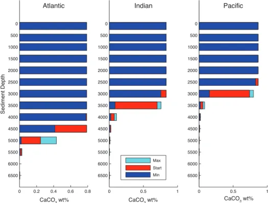
Figure 5 shows the sediment carbonate content for each ocean basin as a function of depth, with colors indicating the starting (red), maximum (light blue), and minimum (dark blue) values that were recorded in each depth box. The deep boxes are most perturbed because they are directly affected by the movement of the CCD. In addition, sediments in the deep Atlantic are perturbed more than those in the Pacific or Indian basins because the CCD is deeper in the Atlantic. Far more carbon enrichment occurs in the Atlantic; for example, the 5000 m box starts at 22 % carbonate and during the run increases to close to 50 %.
Figure 6 shows the time derivative of global TA for the aforementioned case. The red curve accounts for the known contributions of TA from weathering feedbacks and there-fore depicts the alkalinity flux that is due to the dissolution and subsequent burial of marine carbonates. Where the red curve is positive, it denotes a net dissolution of carbonates; where it is negative, it denotes a net burial of carbonates.The peak fluxes occur about 3600 years after emission onset, si-multaneous with the peak in the average surface pH. Figure 6 shows the dominance of sediment processes in determining
the total alkalinity. In this simulation ≈80% of the
maxi-mum flux of alkalinity to the ocean is due to the dissolution of sediments, which helps to explain the relatively minor role played by weathering in determining the peak atmospheric carbon dioxide.
Figure 7 shows theδ13C isotope signature for the
atmo-sphere and ocean boxes as a function of time for the case of
E=1000 PgC andD=5 kyr. The signatures of the surface,
0 1 2 3 4 5 6 7.6
7.74 7.88 8.02 8.16 8.3
pH
6 3.12
3.152 3.184 3.216 3.248 3.28
TA [x 10
18
mol]
Ocean Basin pH & Global TA
0 1 2 3 4 5 6
0 20 40 60 80 100
Atlantic Sediments
CaCO
3
[wt %]
0 1 2 3 4 5 6
0 5 10 15 20 25
Temperature [
oC]
Average Ocean Temperatures
4500 m
5000 m
5500 m (a)
(b) (c)
S
M
D H Atm SA
SI SP MA MI MP DA DI DP H pH
Log 10Time [yrs] Log 10Time [yrs]
Log 10Time [yrs]
TA
Figure 4.System variables as a function of time for the case ofE=1000 PgC andD=5 kyr. Shaded regions indicate time of emission.
(a)Thin lines are pH for the surface (S), intermediate (M), and deep (D) ocean boxes in the Atlantic (A), Indian (I), and Pacific (P) basins. Thick solid line is the global ocean total alkalinity (TA).(b)CaCO3wt % of sediment boxes within the Atlantic Basin.(c)Temperature for atmosphere (Atm) and high-latitude boxes (H). Surface (S), intermediate (M), and deep (D) ocean temperatures are averages across basins..
0 0.2 0.4 0.6 0.8 0
500
1000
1500
2000
2500
3000
3500
4000
4500
5000
5500
6000
6500
Se
d
ime
n
t
D
e
p
th
CaCO3 wt%
Atlantic
0 0.5 1
0
500
1000
1500
2000
2500
3000
3500
4000
4500
5000
5500
6000
6500
Indian
0 0.5 1
0
500
1000
1500
2000
2500
3000
3500
4000
4500
5000
5500
6000
6500
Pacific
Max
Start
Min
CaCO3 wt%
CaCO3 wt%
0 1 2 3 4 5 6 −0.5
0 0.5 1 1.5 2 2.5 3
TA Flux From Sediments
T
A
F
lu
x
[
x
1
0
1
3 Mo
l/
yr]
Log 10Time [yrs]
Figure 6.Time rate of change in global total alkalinity (TA) for the case ofE=1000 PgC andD=5 kyr. Shaded region indicates time of emission. Blue curve is the time rate of change in global ocean TA. Red curve shows the blue curve minus the TA flux that is due to weathering feedbacks.
0 1 2 3 4 5 6
−8 −6 −4 −2 0 2 4
Log10 Time [yrs]
δ
1
3C
[p
e
r
m
ill]
Atm H
D
M S
Figure 7.Carbon-13 isotope signature for the atmosphere (Atm) and ocean boxes as a function of time for the case ofE=1000 PgC and D=5 kyr. The surface (S), intermediate (M), and deep (D) boxes were averaged for all basins. H is high-latitude box. Shaded region indicates time of emission.
4 Power law scalings
Table 1 compares two cases which differ in D and E but
share the same 1R. If the system response was linear, the
perturbations in these two cases would be in proportion to
E, i.e., they differ twenty-fold in their response. However,
Table 1.Comparison of cases.
1V Units Case 1 Case 2 Case 2 : Case 1 D=1 kyr D=100 kyr
E=1000 PgC E=20 000 PgC
TCatm PgC 158.313 2123.627 13.41 TCocn PgC 0.1681×10⁴ 3.0729×10⁴ 18.28 TA mol 0.1354×10¹⁸ 2.4707×10¹⁸ 18.25
δ13Catm ‰ 1.009 3.550 3.52
δ13CS ‰ 1.036 4.775 4.61
δ13CM ‰ 0.686 4.955 7.22
δ13CD ‰ 0.873 12.188 13.96
Table 1 shows that none of these variables are in the
propor-tion of 20:1. For a nonlinear response that depends only on
1R, these variables would be in constant proportion other
than 20:1. This is not the case either. Accordingly, a more
general formulation is needed to systematize these results. A power law relationship between the peak change in
a system variable1V and the total magnitude and duration
of the emission event shown in Fig. 1 can be written as
1V =γ DαEβ, (6)
where the coefficient γ and the exponents α and β
assume different values for each system variable.
Alternatively, Eq. (6) can be written in terms of
emission rate using1R=2E/D:
1V =2−βγ Dα+β1Rβ =2αγ Eα+β1R−α. (7)
If the peak change in1V depends only on the peak
emis-sions rate,1R, thenα= −βin Eqs. (6) and (7). Other
Table 2.Summary of weathering strength variations considered.
nsi 0.20∗ 0.20 0.20 0.20 0.20 0.025 0.10 0.40 2.0
ncc 0.40∗ 0.025 0.05 0.80 2.0 0.40 0.40 0.40 0.40
∗indicates LOSCAR default values.
Table 3.Variable definitions and symbols used.
Variable Symbol Units
Atmosphere atm NA
Ocean ocn NA
Sediments sed NA
High-latitude, Atlantic, Indian, Pacific basins H, A, I, P NA Surface-, intermediate-, deep-ocean boxes S, M, D NA
Emissions rate R PgC yr−1
Emissions duration D yr
Total emissions E PgC
System variable V Varies
Coefficient γ Varies
Duration scaling exponent α ND
Emissions scaling exponent β ND
Global total alkalinity TA mol
pH pH ND
Temperature T ◦C
Sediment carbonate weight % % CaCO3 ND
Time t yr
Total atmospheric carbon TCatm PgC
Total oceanic carbon TCocn PgC
Carbon-13 isotope δ13C ‰
Volcanic degassing flux Fvc PgC yr−1 Air–Sea gas exchange flux Fgas PgC yr−1 Carbonate weathering flux Fcc PgC yr−1 Silicate weathering flux Fsi PgC yr−1
Emissions flux R′ PgC yr−1
Silicate weathering exponent nsi ND Carbonate weathering exponent ncc ND Calcite compensation depth CCD km
Carbonate ion CO2−3 mol
peak values depend on the actual time-varying emissions rate
R′(t)=R(t)−Ro. Our scaling analysis considers only the
peak values of the perturbed variables. To determine global ocean carbon content, we multiplied the dissolved inorganic carbon (DIC) concentrations in each of the ocean boxes by their prescribed volumes to obtain the total mass of carbon in each box. We then summed over all the ocean boxes to
define the variable TCocn. We used this same procedure to
determine the global ocean total alkalinity. For the
analy-sis of temperature,δ13C, and pH, we calculated the
volume-weighted averages for the surface-, intermediate-, and deep-ocean boxes, respectively. Once peak variables were
ob-tained, we performed a regression analysis againstDandE
for each system variable.
The results of this procedure for TCatm, TCocn, and TA
are shown in Figs. 8–10. Figures 8a, 9a, and 10a show the
unscaled peak changes in these variables vs.Efor different
Dvalues.1TCatmhas a distinct dependence onD, whereas
1TCocn and1TA have virtually none. Figures 8b, 9b, and
10b show the peak changes scaled according to Eq. (6). The peak changes in Figs. 9b and 10b vary linearly with
emis-sions sizeE, and accordingly the scaled results collapse to
a power law fit with negligible deviation. In Fig. 8b,
how-ever, the power law behavior of the1TCatmfit is limited to
the range 102< E <104PgC. The deviation at the upper end of this range is due to the fact that the carbonate sediments cannot be dissolved without limit; at some point the accessi-ble carbon reservoir in the sediments becomes exhausted.
Tables 4–6 give the results of our power law scalings for the modern LOSCAR configuration in terms of best-fitting
values for the exponentsαandβ, the preexponential
coeffi-cientγ, and theRvalue of the fit. Althoughα <0 andβ >0 for all variables, as expected, large differences in some of
the exponents are evident. For example, TCatm and TCocn
have very different dependences on durationD, with the
at-mosphere exponent having a value ofα= −0.289 and the
ocean exponent having a value ofα= −0.0035. These
vari-ables also have differentβdependences, with the atmosphere
exponent having a value of β=1.174 and the ocean
hav-ing a relatively weaker exponent value ofβ=0.982. Note,
however, thatα+β≃1 for both of these, as well as for TA.
Ocean and atmosphere temperatures generally have smaller
βvalues andα+βin the range 0.6–0.8.
Scalings for theδ13C variables in the atmosphere and in
the upper and intermediate-ocean boxes show dependence on duration, while the deep-ocean box shows negligible de-pendence. This result suggests that by using the isotopic sig-natures from organisms from different depths that were de-posited at the same time, one could explicitly solve for the
EandDthat produced that particular isotopic excursion. In
general, the duration dependence of ocean variables weakens going downward from the surface.
5 Power law scalings for the Paleocene and Eocene
Table 4.Power law scalings for modern configuration, global variables, and1V=γ DαEβ.Din yr andEin PgC.
V Units γ α β Rvalue
TCatm PgC 0.805 −0.289 1.174 0.988 Tatm ◦C 2.580×10⁻² −0.200 0.794 0.964
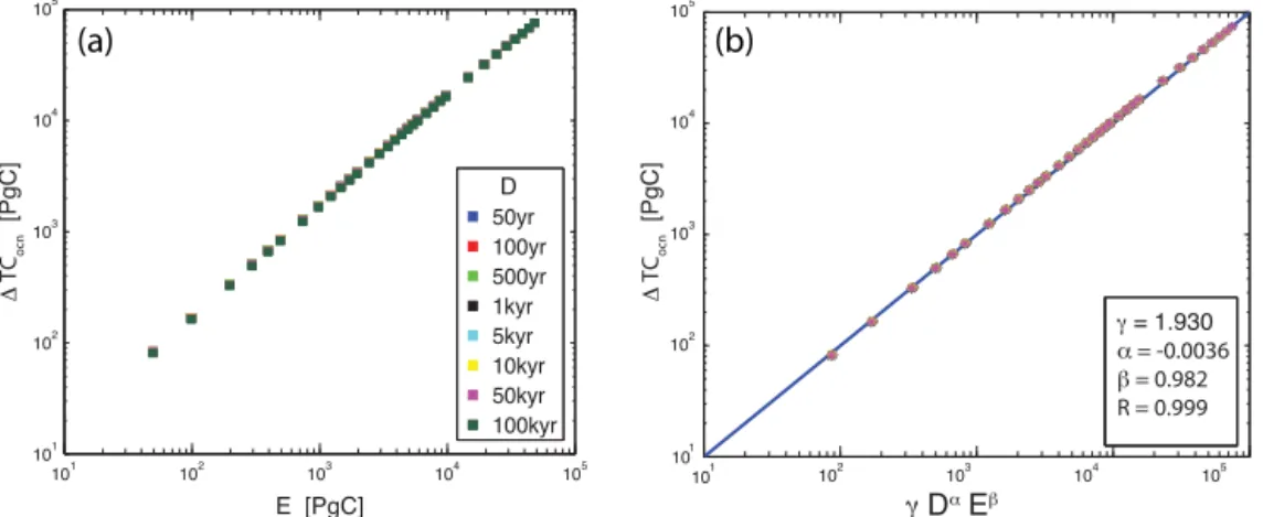
TCocn PgC 1.930 −3.556×10⁻³ 0.982 0.999
TA mol 1.561×10¹⁴ −3.467×10⁻³ 0.981 0.999 Max TCO23− mol 2.021×10¹² −1.775×10⁻⁴ 0.965 0.998 Min TCO23− mol 3.201×10¹⁴ −0.209 0.736 0.899
Table 5.Power law scalings for modern configuration,δ13C variables,1V=γ DαEβ.Din [yr] andEin [PgC].
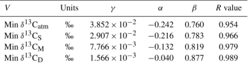
V Units γ α β Rvalue Minδ13Catm ‰ 3.852×10⁻² −0.242 0.760 0.954
Minδ13CS ‰ 2.907×10⁻² −0.216 0.783 0.966
Minδ13CM ‰ 7.766×10⁻³ −0.132 0.819 0.979
Minδ13CD ‰ 1.566×10⁻³ −0.040 0.877 0.989
These simulations were initialized using steady-state
pre-PETM conditions with an atmosphericpCO2=1000 ppmv,
corresponding to a total atmosphere carbon content of
TCatm=2200 PgC. The initial total carbon content of the
global oceans was TCocn=34 196 PgC, and the initial global
ocean total alkalinity (TA) was TA=2.7895×10¹⁸mol. The
idealized emission events began 100 years after startup. The run lengths, like in the modern configuration, also spanned 5 Myr in order to ensure that final steady-state conditions were reached. Tables 7–9 give the results of our power law scalings for this configuration.
A comparison of the scalings shows that the responses to transient perturbations are qualitatively similar across the two climates. Figures 13–15 show the correlations of peak perturbations in the two configurations. For most emission events the correlation is high; however, there are systematic deviations for some variables. For example, the paleo-ocean systematically takes up less carbon than the modern ocean (Fig. 13b), leaving more in the atmosphere (Fig. 13a). This is likely to be due to higher paleo-temperatures and lower alkalinities resulting in weaker ocean buffering capacity. The changes in pH, however, are systematically larger in the mod-ern ocean compared to the paleo-ocean(Fig. 14a). The rel-atively small changes in carbonate chemistry are unlikely
to explain the systematics (doublingpCO2with the
paleo-surface-temperature of 25◦C and an alkalinity of 2000 µM
gives almost the same change in pH as a modern temperature
of 20◦C and an alkalinity of 2300 µM). The differences in
pH are possibly due to differences in the carbonate weather-ing feedbacks or because the ocean circulation is stronger in the paleo-version. Carbon-13 anomalies tend to be smaller at the surface in the paleo-version, but the deep anomalies are essentially identical in both (Fig. 15).
6 Scaling law exponent sensitivity to variations in weathering feedbacks
Examples of system variable sensitivity to nsi and ncc, within LOSCAR, have been explored in previous studies (Uchikawa and Zeebe, 2008; Komar and Zeebe, 2011), but the relative range of the values studied was restricted by only consider-ing enhanced feedbacks due to nominal values of these pa-rameters (Zeebe, 2012b). Here we consider a broader range of these values in the modern LOSCAR configuration to
de-termineαandβsensitivity to large variations in the strength
of these feedbacks. Table 2 shows the cases considered.
Figure 11 shows the resultingαandβvalues for the cases
in Table 2 for the peak changes in TCatm, TCocn, and TA.
Figure 11a shows that, as ncc increases while nsi is held at
the default value, the resultingα values for TCatm become
more negative. Increasing nsi while holding ncc at the
de-fault value also results in more negativeαvalues. Figure 11b
shows that, as ncc increases while nsi is held at the default
value, the resulting β values for TCatm monotonically
de-crease. Increasing nsi while holding ncc at the default value
also results in smaller β values. Figure 11c shows that. as
ncc increases while nsi is held at the default value, the
re-sulting α values for TCocn decrease negligibly. Increasing
nsi while holding ncc at the default value also results
neg-ligible changes inα values. Figure 11d shows that, as ncc
increases while nsi is held at the default value, the resulting
β values for TCocn monotonically increase. Increasing nsi
while holding ncc at the default value produces
monotoni-cally decreasingβ values. Figure 11e shows that increasing
ncc while holding nsi at the default value yields negligible
changes inαvalues for TA. Increasing nsi while holding ncc
at the default value also results in negligible changes in the
Table 6.Power law scaling for modern configuration, ocean boxes, and1V =γ DαEβ.Din yr andEin PgC.
V Units γ α β Rvalue
TAS PgC 4.621×10⁻² −3.508×10⁻³ 0.982 0.999 TAM PgC 4.122×10⁻¹ −3.513×10⁻³ 0.982 0.999
TAD PgC 1.385 −3.467×10⁻³ 0.983 0.999
TAHL PgC 1.271×10⁻² −3.423×10⁻³ 0.982 0.999
TDICS PgC 6.436×10⁻² −1.776×10⁻² 0.959 0.998
TDICM PgC 0.420 −3.60×10⁻³ 0.982 0.999
TDICD PgC 1.454 −3.541×10⁻³ 0.982 0.999
TDICHL PgC 1.350×10⁻² −4.23×10⁻³ 0.979 0.999 TS ◦C 2.473×10⁻² −0.196 0.795 0.964 TM ◦C 1.318×10⁻² −0.157 0.824 0.968
TD ◦C 4.888×10⁻³ −0.098 0.863 0.979
Min pHS ND 2.365×10⁻³ −0.249 0.818 0.962
Min pHM ND 2.050×10⁻³ −0.211 0.799 0.940
Min pHD ND 5.320×10⁻⁴ −0.134 0.853 0.968
Min CO23 S− mol 5.083×10¹³ −0.336 0.744 0.887 Min CO23 M− mol 2.356×10¹⁴ −0.256 0.684 0.864 Min CO23 D− mol 1.522×10¹⁴ −0.191 0.751 0.912 Min CO23 HL− mol 8.867×10¹² −0.289 0.711 0.894 Max CO23 S− mol 2.473×10¹¹ −3.223×10⁻³ 0.902 0.994 Max CO23 M− mol 9.146×10¹¹ −1.595×10⁻⁴ 0.946 0.998 Max CO23 D− mol 9.574×10¹¹ 8.321×10⁻⁴ 0.980 0.998 Max CO23 HL− mol 2.013×10¹⁰ −9.039×10⁻⁴ 0.910 0.992 Max CCDA km 2.749×10⁻⁴ −1.103×10⁻² 0.837 0.934
Max CCDI km 1.279×10⁻⁵ −1.298×10⁻² 1.210 0.955
Max CCDP km 4.798×10⁻⁶ −9.784×10⁻³ 1.297 0.961
Min CCDA km 1.131×10⁻² −0.178 0.734 0.904
Min CCDI km 6.233×10⁻⁴ −0.220 1.046 0.896
Min CCDP km 1.908×10⁻⁴ −0.189 1.135 0.896
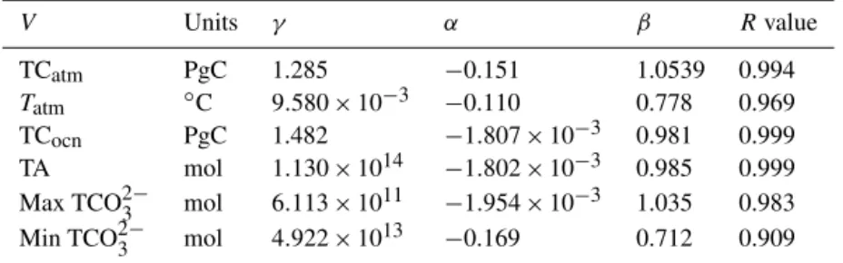
Table 7.Power law scalings for Paleocene–Eocene configuration, global variables, and1V =γ DαEβ.Din yr andEin PgC.
V Units γ α β Rvalue
TCatm PgC 1.285 −0.151 1.0539 0.994 Tatm ◦C 9.580×10⁻³ −0.110 0.778 0.969
TCocn PgC 1.482 −1.807×10⁻³ 0.981 0.999
TA mol 1.130×10¹⁴ −1.802×10⁻³ 0.985 0.999 Max TCO23− mol 6.113×10¹¹ −1.954×10⁻³ 1.035 0.983 Min TCO23− mol 4.922×10¹³ −0.169 0.712 0.909
held at the default value, the resultingβvalues for TA
mono-tonically increase, similar to the behavior in Fig. 11d. More-over, increasing nsi while holding ncc at the default value
yields smallerβ values, like those in Fig. 11d. In summary,
Fig. 11 shows that β values are relatively more sensitive to
changes in weathering strengths.
7 Discussion
Table 8.Power law scalings for Paleocene and Eocene configuration,δ13C variables, and1V =γ DαEβ.Din yr andEin PgC.
V Units γ α β Rvalue Minδ13Catm ‰ 2.005×10⁻² −0.199 0.777 0.963
Minδ13CS ‰ 1.776×10⁻² −0.178 0.783 0.969
Minδ13CM ‰ 5.243×10⁻³ −0.099 0.819 0.981
Minδ13CD ‰ 1.447×10⁻³ −0.031 0.876 0.990
Table 9.Power law scaling for Paleocene and Eocene configuration, ocean boxes, and1V=γ DαEβ.Din yr andEin PgC.
V Units γ α β Rvalue
TAS PgC 0.035 −1.821×10⁻³ 0.983 0.999
TAM PgC 0.304 −1.837×10⁻³ 0.984 0.999
TAD PgC 1.013 −1.810×10⁻³ 0.985 0.999
TAHL PgC 8.414×10⁻³ −1.730×10⁻³ 0.983 0.999
TDICS PgC 0.037 −1.811×10⁻³ 0.980 0.999
TDICM PgC 0.328 −1.834×10⁻³ 0.981 0.999
TDICD PgC 1.103 −1.855×10⁻³ 0.982 0. 999
TDICHL PgC 9.032×10⁻³ −1.823×10⁻³ 0.982 0.999 TS ◦C 9.180×10⁻³ −0.108 0.780 0.969 TM ◦C 6.767×10⁻³ −8.741×10⁻² 0.792 0.970 TD ◦C 4.251×10⁻³ −6.027×10⁻² 0.812 0.976
Min pHS ND 1.063×10⁻³ −0.151 0.782 0.965
Min pHM ND 8.839×10⁻⁴ −0.136 0.746 0.949
Min pHD ND 3.203×10⁻⁴ −0.095 0.812 0.970
Min CO23 S− mol 9.639×10¹² −0.190 0.673 0.906 Min CO23 M− mol 2.637×10¹³ −0.205 0.649 0.881 Min CO23 D− mol 2.537×10¹³ −0.165 0.736 0.916 Min CO23 HL− mol 1.497×10¹² −0.184 0.672 0.908 Max CO23 S− mol 1.378×10¹⁰ −2.215×10⁻³ 1.051 0. 948 Max CO23 M− mol 1.914×10¹¹ −1.979×10⁻³ 1.030 0.987 Max CO23 D− mol 4.115×10¹¹ −2.081×10⁻³ 1.034 0.982
Max CO23 HL− mol 1.373×10⁹ −2.000×10⁻³ 1.070 0.927 Max CCDA km 4.563×10⁻⁴ −1.441×10⁻³ 0.825 0.978
Max CCDI km 8.724×10⁻⁵ −1.214×10⁻³ 1.007 0.974
Max CCDP km 1.772×10⁻⁵ −1.833×10⁻³ 1.192 0.955
Max CCDT km 4.472×10⁻⁵ −1.784×10⁻³ 1.133 0.946
Min CCDA km 8.918×10⁻³ −0.124 0.666 0.911
Min CCDI km 2.968×10⁻³ −0.166 0.805 0.888
Min CCDP km 1.409×10⁻⁴ −0.173 1.109 0.904
Min CCDT km 4.877×10⁻⁴ −0.202 0.986 0.840
1. Why is the dependence on weathering so weak?
2. What controls the maximum in CO2?
3. What does this imply about additional feedbacks in the system?
Considerable insight can be gained into how the maximum
pCO2is set by noting that the bicarbonate ion concentration
at equilibrium is given by
[HCO−3] =kH k1pCO2
[H+] , (8)
wherekHis the Henry’s law coefficient,k1andk2are
disso-ciation coefficients, and [H+] is the hydrogen ion
concentra-tion. Similarly, the equilibrium carbonate ion concentration is given by
[CO23−] =kH k1k2pCO2
(a) (b)
γ = 0.805
α = -0.289
β = 1.174
R = 0.988 D
Δ
TC
atm
[PgC]
1
102 103 104 105
1 102 103 104 105
γ Dα Eβ
10 10
1 102 103 104 105
E [PgC]
10
Δ
TC
atm
[PgC]
101 102 103 104 105
50yr 100yr 500yr 1kyr 5kyr 10kyr 50kyr 100kyr
Figure 8.(a)Peak changes in the modern atmospheric total carbon content as a function of total emission,E, for various durations,D.
(b)Multivariable regression results. Solid line indicates a perfect fit to the predicted scaling. The asterisks are each individual cases.
Δ
TC
ocn
[PgC]
Δ
TC
ocn
[PgC]
1
102 103 104 105 101
102
103
104
105
1
102 103 104 105
1
102 103 104 105
E [PgC] γDα Eβ
10
10 10
(a) (b)
D
50yr 100yr 500yr 1kyr 5kyr 10kyr 50kyr 100kyr
γ = 1.930
α = -0.0036
β = 0.982
R = 0.999
Figure 9.(a)Peak changes in the modern oceanic total carbon content as a function of total emission,E, for various durations,D.(b) Mul-tivariable regression results. Solid line indicates a perfect fit to the predicted scaling. The asterisks are each individual cases.
Then we can solve for thepCO2from Eqs. (8) and (9)
pCO2= k2 kHk1
[HCO−3]2
[CO23−] . (10)
Letting DIC be the dissolved inorganic carbon, ALK the
carbonate alkalinity, and C=kHpCO2 the aqueouspCO2,
we find that
pCO2≈ kH k1
k2
(2DIC−ALK+C)2
(ALK−DIC) (11)
When pCO2 is at a maximum ∂C/∂t is likewise 0 so
that we can find a relationship between ∂DIC/∂t and
∂ALK/∂t.Taking the derivative with respect to time at the
maximumpCO2,
2(2 DIC−ALK+C)
(ALK−DIC)
2∂DIC
∂t − ∂ALK
∂t
−(2DIC−ALK+C)
2
(ALK−DIC)2
∂ALK
∂t − ∂DIC
∂t
=0. (12)
This can be solved to give us
∂ALK
∂t =
3ALK−2DIC+2C
ALK
∂DIC
∂t . (13)
This can also be rewritten as
∂ALK
∂t =
[HCO−3] +4[CO23−]
[HCO−3] +2[CO23−]
∂DIC
∂t (14)
so that the maximum inpCO2is reached when the alkalinity
change is a little higher than the DIC change. Since
101 102 103 104 105
1015
1016
1017
1018
1019
1015 1016 1017 1018 1019
1015
1016
1017
1018
1019
E [PgC]
Δ
TA [mol]
γ Dα Eβ
Δ
TA [mol]
(a) (b)
D
50yr 100yr 500yr 1kyr 5kyr 10kyr 50kyr 100kyr
γ= 1.561e14
α = -0.0035
β = 0.981
R = 0.999
Figure 10.(a)Peak changes in the modern global ocean total alkalinity (TA) as a function of total emission,E, for various durations,D.
(b)Multivariable regression results. Solid line indicates a perfect fit to the predicted scaling. The asterisks are each individual cases.
we can rewrite this as
∂ALK/∂t
∂DIC/∂t =θ=
1+4k2/[H+] 1+2k2/[H+]
. (16)
There are two possible ways for ∂pCO2/∂t to equal 0 in
Eq. (11). The first is the equilibrium regime where the emissions occur over very long timescales and the sur-face changes in TDIC and ALK mirror the ocean-average changes. This is the regime in which we would expect to find a strong dependence on weathering parameters. However, as can be seen from looking at Fig. 12, our transient simulations
are characterized by a dynamicbalance, where both TDIC
and TA are changing. This dynamic balance means that it is the growth of alkalinity within the ocean that brings
atmo-sphericpCO2into balance. Examiningθat the time of
max-imumpCO2(Fig. 12a) shows that the two terms are
approx-imately the same for all the runs with durations of 10 000, 50 000 and 100 000 years. For surface temperatures of around 20◦C,k
2≈10−9so that the ratio between alkalinity and DIC
change is around about 1.2 at low emissions. As the pH in-creases for longer timescales, this ratio drops towards 1.
For short durations, by contrast, the peak is found whenθ
is very small. Rather than carbonate reactions being impor-tant, what matters is the ability of the ocean circulation to move carbon away from the surface. A careful examination of these cases shows that the bulk of added carbon dioxide resides in the atmosphere.
The relatively weak dependence of θ on total emissions
obscures an interesting difference between short- and
long-duration pulses. For short-long-duration pulses,θincreases as the
emissions increase. As more and more carbon is added to the system over short periods of time, more of it reacts with calcium carbonate and increases ocean alkalinity. However, for the long-duration simulations, the dependence runs in the opposite direction, with higher emissions showing less com-pensation from alkalinity.
To first order, a situation in which the growth rates in TDIC and TA are equal is what one would expect in a system with-out burial, where the additional carbon added to the atmo-sphere reacts with silicate rocks and the additional alkalinity ends up accumulating in the ocean. Such a situation would also be expected to have a strong dependence on weathering parameters. However, in LOSCAR the dominant flux of al-kalinity is often from the sediments to the ocean. This flux will grow not just because the deep-ocean pH decreases but because more sediments are mobilized as this happens.
At intermediate durations the picture becomes much more complicated. There appears to be an optimal emission for maximizing interactions with the sediments. The reasons for this are unclear, but it is striking that the timescales involved are similar to the timescales for ocean overturning.
Note that the discretization of the deep ocean into a fixed number of boxes introduces some step-like behavior into the volume of sediments mobilized, which can be seen in Fig. 12b. The fact that less sediment is available for
inter-action as the lysocline shallows may explain part of whyθ
drops at high emission in Fig. 12b. In any case, we expect the sediment alkalinity flux to have a functional dependence on the perturbation DIC, which is linear or superlinear, im-plying that it has the potential to overwhelm the rather weak
dependence onpCO2.
Our results suggest future sensitivity studies. For exam-ple, what differences between the Paleocene and Eocene and modern world produce different scaling laws? Answers might be found in different ocean circulation patterns or dif-ferent hypsometric distributions, which would then
deter-mine the amount of sediment available to react with CO2.
Additionally, the strong role played by the oceanic carbon-ate budget suggests additional feedbacks involving the bio-logical pump. In the version of LOSCAR used here, the re-moval of organic material from the surface layer is primarily controlled by high-latitude nutrients and the ocean
0 0.5 1 1.5 2 −0.5
−0.4 −0.3 −0.2 −0.1 0
0.1 Δ
TA
Weathering Exponent
α
CC SI
0 0.5 1 1.5 2
0.75 0.8 0.85 0.9 0.95 1 1.05 1.1 1.15 1.2
1.25 Δ
TA
Weathering Exponent CC SI
β
0 0.5 1 1.5 2
Weathering Exponent 0.8
0.9 1 1.1 1.2
β
ΔTC
atm
−0.5 −0.4 −0.3 −0.2 −0.1 0 0.1
α
0 0.5 1 1.5 2
Weathering Exponent
ΔTC
atm
0 0.5 1 1.5 2
Weathering Exponent −0.5
−0.4 −0.3 −0.2 −0.1 0 0.1
α
ΔTC
ocn
0 0.5 1 1.5 2
Weathering Exponent 0.8
0.9 1 1.1 1.2
β
ΔTC
ocn
(a) (b)
(c) (d)
(e) (f )
Figure 11.Sensitivity of scaling results to variations in weathering exponents. Dashed lines indicate default LOSCAR exponent values (ncc=0.40; nsi=0.20).(a, b)Peak total atmospheric carbon;(c, d)peak total ocean carbon;(e, f)peak global total alkalinity (TA).
θ
101 102 103 104 105
Duration [yrs]
101 102 103 104 105
Emission [PgC]
(a)
(b)
0.2 0.4 0.6 0.8 1.0 1.2
0.2 0.4 0.6 0.8 1.0 1.2
θ 50 yr
100 yr 500 yr 1 kyr 5 kyr 10 kyr 50 kyr 100 kyr
0 1 2 3 4 5 6
7x 10⁴
0 1 2 3 4 5 6 7 8
0 1 2 3 4 5 6
7x 10
4
0 1 2 3 4 5 6 7x 10
4 x 10⁴
Modern Scaling Modern Scaling
Paleo Scaling
Paleo Scaling
ΔTCatm [PgC] Δ TCocn [PgC]
Increasing Duration
Same Color = Same Total Emissions (E) Same Color = Same Total Emissions (E)
E=50 000 PgC
E=25 000 PgC
E=10 000 PgC
E=5 000 PgC
E=50 000 PgC
E=25 000 PgC
E=10 000 PgC
E=5 000 PgC
E=1 000 PgC
(a) (b)
Figure 13.Correlation between peak perturbations for modern and paleo-scalings.(a)Total atmospheric carbon.(b)Total oceanic carbon. Same color denotes same total emissions.
0 1 2 3 4 5 6 0 1 2 3 4 5 6
0 1 2 3 4 5 6
0 1 2 3 4 5 6 7x 10
18
7x 10
18
Modern Scaling Modern Scaling
Paleo Scaling Paleo Scaling
Δ pH Surface Δ Global TA [mol]
Increasing Duration
Same Color = Same Total Emissions (E) Same Color = Same Total Emissions (E)
E=50 000 PgC
E=25 000 PgC
E=10 000 PgC
E=5 000 PgC E=1 000 PgC E=50 000 PgC
E=25 000 PgC
E=10 000 PgC
E=5 000 PgC
(a) (b)
Figure 14.Correlation between peak perturbations for modern and paleo-scalings.(a)Surface pH.(b)Total global alkalinity. Same color denotes same total emissions.
Additionally, the rain ratio of particulate inorganic carbon to organic carbon is held constant. All of these are likely to vary in the real world.
However, it should also be noted that a robust connection between these changes in the biological pump and climate re-mains uncertain. For example, today the deep ocean receives water injected from the North Atlantic, which in the modern world has relatively low surface nutrients, and the Southern Ocean, which has relatively high surface nutrients. As noted by Marinov et al. (2008), changes in the balance of deep wa-ters formed in these regions can significantly alter the car-bon stored by the biological pump in the deep ocean so that a slowdown in circulation may produce either increased or decreased storage of carbon (with corresponding changes in deep-ocean acidity). While one might expect the total level of vertical exchange to decrease as atmospheric carbon diox-ide increases, it is much less clear how the balance between the two source regions would change.
Similarly, there are open questions regarding the rain ra-tio. While it does seem likely that this value will be a func-tion of carbon saturafunc-tion state, it is not clear what the de-pendence should be. While some calcifying organisms like corals (Langdon et al., 2000) and pteropods (Fabry et al., 2008) tend to grow more slowly under higher levels of carbon dioxide, other calcifying organisms such as coccolithophores may become more abundant (S. Rivero-Calle, personal com-munication, 2014).
See the Supplement for an example of how the scaling laws, which are based on an idealized emission shape, may be used to estimate the peak perturbations from more realis-tic fossil fuel emission scenarios.
0 10 20 30 40 50 60 0
10 20 30 40 50 60
Modern Scaling
0 2 4 6 8 10 12 14 16 18 20 0
2 4 6 8 10 12 14 16 18 20
Modern Scaling
Paleo Scaling Paleo Scaling
Δ δ13C Deep [per mill]
Δ δ13C Surface [per mill]
Increasing Duration
Same Color = Same Total Emissions (E) E=1 000 PgC Same Color = Same Total Emissions (E)
E=50 000 PgC
E=25 000 PgC
E=10 000 PgC
E=5 000 PgC
E=50 000 PgC
E=25 000 PgC
E=10 000 PgC
E=5 000 PgC
(a) (b)
Figure 15.Correlation between peak perturbations for modern and paleo-scalings.(a)Surface-ocean carbon-13 anomalies.(b)Deep-ocean carbon-13 anomalies. Same color denotes same total emissions.
Acknowledgements. This research has been supported by
National Science Foundation Frontiers of Earth System Dynamics grant EAR-1 135 382. Special thanks to Richard Zeebe for making the LOSCAR code available.
Edited by: A. Haywood
References
Archer, D., Eby, M., Brovkin, V., Ridgwell, A., Cao, L., Mikolajew-icz, U., and Caldeira, K., Matsumoto, K., Munhoven, G., Mon-tenegro, A., and Tokos, K.: Atmospheric lifetime of fossil fuel carbon dioxide, Annu. Rev. Earth Pl. Sc., 37, 117–134, 2009. Berner, R. A. and Caldeira, K.: The need for mass balance and
feed-back in the geochemical carbon cycle, Geology, 25, 955–956, 1997.
Berner, R. A. and Kothavala, Z.: GEOCARB III: a revised model of atmospheric CO2over Phanerozoic time, Am. J. Sci., 301, 182–
204, 2001.
Berner, R. A., Lasaga, A. C., and Garrels, R. M.: The carbonate-silicate geochemical cycle and its effect on atmospheric carbon dioxide over the past 100 million years, Am. J. Sci., 283, 641– 683, 1983.
Fabry, V. J., Seibel, B. A., Feely, R. A., and Orr, J. C.: Impacts of ocean acidification on marine fauna and ecosystem processes, ICES J. Mar. Sci., 65, 414–432, 2008.
Komar, N. and Zeebe, R. E.: Oceanic calcium changes from en-hanced weathering during the Paleocene-Eocene Thermal Maxi-mum: no effect on calcium-based proxies, Paleoceanography, 26, PA3211, doi:10.1029/2010PA001979, 2011.
Komar, N., Zeebe, R. E., and Dickens, G. R.: Understanding long-term carbon cycle trends: the late Paleocene through the early Eocene, Paleoceanography, 28, 650–662, 2013.
Langdon, C., Takahashi, T., Sweeney, C., Chipman, D., and Atkin-son, J.: Effect of calcium carbonate saturation on the calcification rate of an experimental coral reef, Global Biogeochem. Cy., 14, 639–654, 2000.
Marinov, I., Gnanadesikan, A., Sarmiento, J. L., Toggweiler, J. R., Follows, M., and Mignone, B. K.: Impact of oceanic cir-culation on biological carbon storage in the ocean and at-mospheric pCO2, Global Biogeochem. Cy., 22, GB3007, doi:10.1029/2007GB002958, 2008.
Matsumoto, K., Sarmiento, J. L., Key, R. M., Aumont, O., Bullister, J. L., Caldeira, K., Campin, J.-M., Doney, S. C., Drange, H., Dutay, J.-C., Follows, M., Gao, Y., Gnanade-sikan, A., Gruber, N., Ishida, A., Joos, F., Lindsay, K., Maier-Reimer, E., Marshall, J. C., Matear, R. J., Monfray, P., Mouchet, A., Najjar, R., Plattner, G.-K., Schlitzer, R., Slater, R., Swathi, P. S., Totterdell, I. J., Weirig, M.-F., Yamanaka, Y., Yool, A., and Orr, J. C.: Evaluation of ocean carbon cycle mod-els with data-based metrics, Geophys. Res. Lett., 31, L07303, doi:10.1029/2003GL018970, 2004.
McKay, D. I., Tyrrell, T., Wilson, P. A.,and Foster, G. L.: Estimating the impact of the cryptic degassing of Large Igneous Provinces: A mid-Miocene case-study, Earth Planet. Sci. Lett., 403, 254– 262, 2014.
Pälike, H., Lyle, M. W., Nishi, H., Raffi, I., Ridgwell, A., Gam-age, K., Klaus, A., Acton, G., Anderson, L., Backman, J., Bal-dauf, J., Beltran, C., Bohaty, S. M., Bown, P., Busch, W., Chan-nell, J. E. T., Chun, C. O. J., Delaney, M., Dewangan, P., Dunk-ley, J. T., Edgar, K. M., Evans, H., Fitch, P., Foster, G. L., Gussone, N., Hasegawa, H., Hathorne, E. C., Hayashi, H., Her-rle, J. O., Holbourn, A., Hovan, S., Hyeong, K., Iijima, K., Ito, T., Kamikuri, S.-I., Kimoto, K., Kuroda, J., Leon-Rodriguez, L., Malinverno, A., Moore, T. C., Murphy, B. H., Murphy, D. P., Nakamura, H., Ogane, K., Ohneiser, C., Richter, C., Robin-son, R., Rohling, E. J., Romero, O., Sawada, K., Scher, H., Schneider, L., Sluijs, A., Takata, H., Tian, J., Tsujimoto, A., Wade, B. S., Westerhold, T., Wilkens, R., Williams, T., Wil-son, P. A., Yamamoto, Y., Yamamoto, S., Yamazaki, T., and Zeebe, R. E.: A Cenozoic record of the equatorial Pacific car-bonate compensation depth, Nature, 488, 609–614, 2012. Paquay, F. S. and Zeebe, R. E.: Assessing possible consequences of
ocean liming on ocean pH, atmospheric CO2concentration and
Ridgwell, A. and Hargreaves, J.: Regulation of atmospheric CO2
by deep-sea sediments in an Earth System Model, Global Bio-geochem. Cy., 21, GB2008, doi:10.1029/2006GB002764, 2007. Ridgwell, A., Hargreaves, J. C., Edwards, N. R., Annan, J. D., Lenton, T. M., Marsh, R., Yool, A., and Watson, A.: Marine geo-chemical data assimilation in an efficient Earth System Model of global biogeochemical cycling, Biogeosciences, 4, 87–104, doi:10.5194/bg-4-87-2007, 2007.
Sarmiento, J. L. and Gruber, N.: Ocean Biogeochemical Dynamics, Princeton University Press, Princeton, NJ, 2006.
Sarmiento, J. L., Hughes, T. M. C., and Stouffer, R. J.: Simulated re-sponse of the ocean carbon cycle to anthropogenic climate warm-ing, Nature, 393, 245–249, 1998.
Sluijs, A., Zeebe, R. E., Bijl, P. K., and Bohaty, S. M.: A mid-dle Eocene carbon cycle conundrum, Nat. Geosci., 6, 429–434, 2013.
Stuecker, M. F. and Zeebe, R. E.: Ocean chemistry and atmospheric CO2sensitivity to carbon perturbations throughout the Cenozoic, Geophys. Res. Lett., 37, L03609, doi:10.1029/2009GL041436, 2010.
Tjiputra, J. F., Assmann, K., Bentsen, M., Bethke, I., Otterå, O. H., Sturm, C., and Heinze, C.: Bergen earth system model (BCM-C): model description and regional climate-carbon cycle feedbacks assessment, Geosci. Model Dev., 3, 123–141, doi:10.5194/gmd-3-123-2010, 2010.
Uchikawa, J. and Zeebe, R. E.: Influence of terrestrial weathering on ocean acidification and the next glacial inception, Geophys. Res. Lett., 35, L23608, doi:10.1029/2008GL035963, 2008.
Uchikawa, J. and Zeebe, R. E.: Examining possible effects of sea-water pH decline on foraminiferal stable isotopes during the Paleocene-Eocene Thermal Maximum, Paleoceanography, 25, PA2216, doi:10.1029/2009PA001864, 2010.
Walker, J. C. G. and Kasting, J. F.: Effects of fuel and for-est conservation on future levels of atmospheric carbon diox-ide, Palaeogeography, Palaeoclimatology, Paleoecology, Global Planet. Change, 97, 151–189, 1992.
Walker, J. C. G., Hays, P. B., and Kasting, J. F.: A negative feedback mechanism for the long-term stabilization of Earth’s surface tem-perature, J. Geophys. Res., 86, 9776–9782, 1981.
Zachos, J. C., Röhl, U., Schellenberg, S.,Sluijs, S., Hodell, D. A., Kelly, D. C.,Thomas, E., Nicolo, M., Raffi, I., Lourens, L. J., McCarren, H., and Kroon, D.: Rapid Acidification of the Ocean During the Paleocene-Eocene Thermal Maximum, Science, 308, 1611–1615, 2005.
Zeebe, R. E.: History of seawater carbonate chemistry, atmospheric CO2, and ocean acidification, Annu. Rev. Earth Pl. Sc., 40, 141– 165, 2012a.
Zeebe, R. E.: LOSCAR: Long-term Ocean-atmosphere-Sediment CArbon cycle Reservoir Model v2.0.4, Geosci. Model Dev., 5, 149–166, doi:10.5194/gmd-5-149-2012, 2012b.
Zeebe, R. E. and Zachos, J. C.: Long-term legacy of massive carbon input to the Earth system: Anthropocene vs. Eocene, Philos. T. R. Soc. Lond., 371, 20120006, doi:10.1098/rsta.2012.0006, 2013. Zeebe, R. E., Zachos, J. C., Caldeira, K., and Tyrrell, T.: Carbon
emissions and acidification, Science, 321, 51–52, 2008. Zeebe, R. E., Zachos, J. C., and Dickens, G. R.: Carbon dioxide