ABSTRACT: Growth functions with inflection points following a diphasic model, can be adjusted by two approaches using segmented regression or the sum of two functions. In both cases, there are two functions, one for each phase, with inflection and stability points. However, when they are summed, the result is a new function and the points of inflection and stability are dif-ferent from those obtained from using each function individually. A method to determine these points in a diphasic logistics sum of functions is suggested and the results obtained from fitting the models to eucalyptus growth data showed a better fit of the logistic diphasic sum as com-pared with segmented regression and monophasic logistic models.
Keywords: nonlinear models, segmented regression, sum of logistics
Introduction
Monophasic models of linear or non-linear growth are a description of the total growth cycle, from birth to adulthood of the individual, which may be greatly sim-plified. However, multiple growth cycles can be found in the literature (Seber and Wild, 1989) from the begin-ning of the 20th century (Brody and Ragsdale, 1921).
Since then, curve adjustment by multiphasic models has been employed in various areas, such as human height growth (Bock et al., 1973), growth in weight of rats (Koops et al., 1987; Kurnianto et al., 1999), chick-ens (Grossman and Koops, 1988), rice crop biomass (Sheehy et al., 2004) and cows (Mendes et al., 2008; Mendes et al., 2009).
The logistic function has been the one most fre-quently used in multiphasic models due to its properties of symmetry in the growth velocity curve (Koops, 1986; Kurnianto et al., 1999; Mendes et al., 2008). This model may be fitted either by segmented regression (Portz et al., 2000; Robbins et al., 2006) or by the sum of func-tions – the most commonly employed methods (Koops, 1986; Koops and Grossman, 1991; Kurnianto et al., 1999; Özkan, 2004; Nešetřilová, 2005; Mendes et al., 2008; Mendes et al., 2009; Fenner et al., 2013).
In the nonlinear multiphasic model with inflec-tion points, adjusted by the sum of funcinflec-tions, the points are determined in the functions that correspond to each growth phase (Koops, 1986; Koops et al., 1987; Koops and Grossman, 1991; Kurnianto et al., 1999; Mendes et al., 2009; Fenner et al., 2013), but the inflection points of the sum function are not determined
In this study, a methodology for the determina-tion of inflecdetermina-tion and stability points of logistic diphasic models as adjusted by the sum of functions is presented, which are compared with the points obtained by seg-mented regression and the monophasic model.
Materials and Methods
Consider the following logistic models, where α > 0 and γ > 0, fitted to a data set (xi; yi) from observed data,
i = 1, 2, ..., n, where errors are considered independent, normal and homoscedastic, e ~N (0, s2
e).
Model I - monophasic logistic model
yi = F(xi,q) = + ei, Xi = exp(–b –γxi), q = [α b γ]’ (1)
Model II - diphasic logistic model segmented re-gression
yi = F(xi,q) = + ei, X1i = exp(–b1 –γ1xi), if x ≤ι,
yi = F(xi,q) = + ei, X2i = exp(–b2 –γ2xi), if x ≥ι, (2)
q = [αkbkγkι]', k = 1, 2, and ι = abscissa of the intersec-tion point of the two funcintersec-tions.
Model III - diphasic logistic sum of functions
yi = F(xi,q) = + ei, Xki = exp(–bk –γkxi),
q = [αk bk γk]', k = 1, 2. (3)
Residual homoscedasticity is checked by the Breusch-Pagan test (Breusch and Pagan, 1979) and nor-mality by the Shapiro-Wilk test. The residual autocorre-lation is verified by the use of tables for testing random-ness of grouping in a sequence of residual signs (Draper and Smith, 1998)
Adjustments to the models can be checked by the usual criteria for comparing models: the residual mean square of the model, RMS; the square of the correla-tion coefficient between observed and fitted values by the model, r2
y.ŷ (Schinckel and Craig, 2002), and the F
criterion
(4)
where: SSR1 is the sum of the squares of residuals of the model with a smaller number of parameters, SSR2 is the São Paulo State University/IBB − Dept. of Biostatistics, C.P.
510 − 18618-970 − Botucatu, SP − Brazil. *Corresponding author <[email protected]>
Edited by: Marcin Kozak
Inflection and stability points of diphasic logistic analysis of growth
Martha Maria Mischan, José Raimundo de Souza Passos, Sheila Zambello de Pinho*, Lídia Raquel de Carvalho
sum of the squares of residuals of the model with a larger number of parameters, and df1 and df2 are degrees of
free-dom associated with SSR1 and SSR2, respectively; the corrected Akaike Information Criterion:
AICc = AIC + 2p(p+1)/(n-p-1), AIC = nloge(SSR/n) + 2p (5)
where: SSR is the sum of the squares of residuals of the model, and p is the number of model parameters, (Narinc et al., 2010). The Akaike information criterion evaluate whether the model adequately describes the studied pop-ulation: the lower the value, the better the model.
To check the fit of the models in the early growth stage the residual square mean of m values, RSMm, was calculated as follows:
RSMm = (6)
where: yi is the i-th observed value, ŷi is the i-th value estimated by the model and m is the number of observa-tions corresponding to the first phase of the fitted logistic by segmented regression (MII).
The inflection points of the logistic function, de-termined by equating its second order derivative to zero, are obtained by the usual formula (-b/γ; α/2) for model I (-bk/γk; αk/2), k = 1, 2, for model II. In model III, however, the function (3) is a sum and its second order derivative equated to zero:
(7)
is an equation without explicit solution, which makes the problem more complex (Beyene and Ramakrishnan, 2013), though the solution can be approximated by it-erative techniques. In this paper, the Newton-Raphson method is used,in the SAS proc model (Statistical Analysis System, version 9.2).
The abscissas of the inflection points of the diphasic logistic sum of functions, therefore, cannot be determined by common formulas for each plot of (7), since there is no fitted function for each phase, but a sum of two functions in the same phase. The solutions of equation (7), denoted by υ, are contained in the interval τ1 < x < τ2, where τk = -bk/γk, k = 1, 2; this is shown below:
Consider the logistic functions defined for αk > 0, bk < 0 and γk > 0,
yk= , Xk = exp(–bk –γk x) = exp[γk (τk – x)],
τk = –bk/γk, k = 1, 2. (8)
The functions are continuous, differentiable, posi-tive and increasing in the interval (-∞, ∞) and have an in-flection point where x equals τk = –bk/γk. The first order derivatives of yk are continuous, positive and have maxima at x = τk, whose values are the roots of the second order derivative functions:
, (9)
that are continuous, positive in the interval -∞ < x < τk and negative in τk < x < ∞. Then the sum function
, Xk = exp[γk (τk – x)], (10)
is also continuous, differentiable, positive and increasing at (- ∞, ∞). Assuming τ1 < τ2 we have in the interval -∞ < x < τ1, by (8), X1 > 1 and X2 > 1 and by (9), y”1 > 0 and
y”2 > 0. Therefore y” = y”1 + y”2 > 0 in this interval. At the point where x = τ1, X1 = 1, X2 > 1, y”1 = 0, y”2 > 0 and y” > 0.
Then,
in -∞ < x ≤τ1, y” > 0; there are no inflections in y in
this interval. (11)
In the interval τ2 < x < ∞, by (8), 0 < X1 < 1 and 0 < X2 < 1 and by (9), y”1 < 0 and y”2 < 0. Therefore y” < 0 in this interval. At the value where x = τ2, X1 < 1, X2 = 1, y”1 < 0, y”2 = 0 and y” < 0. Then,
where τ2≤ x < ∞, y” < 0; there are no inflections in y
in this interval. (12)
By (11) and (12), as y’’ is continuous on (- ∞, ∞) it follows that there is at least one value of x in the interval (τ1, τ2) where y’’ is equal to zero. This value where x = υ is the abscissa of the inflection point of y in (10).
The stability points of the logistic function, mono or diphasic can be determined by various methods (Pas-sos et al., 2012). The method that equates the fourth-order derivative of the function y to zero is employed here (Mischan et al., 2011):
, X = exp(–b –γx)(13)
which gives the points
[–b–loge(5+2 )]/γ; α/[2(3+ )] (14)
in model I and
{[–bk–loge(5+2 )]/γk; αk/[2(3+ )]}, k = 1, 2 (15)
in model II.
In model III, where there is a sum of functions, the equation
=0,
has no explicit solution. The solution method is the same used for the determination of inflection points.
The models were adjusted using the procedure
model, method=marquardt, from SAS (Statistical Analy-sis System, version 9.2). The options breusch ‘pagan’ and
normal in the proc model were employed to verify the ho-moscedasticity and normality of the residuals. All tests were verified at the significance level of α = 0.05.
Observational growth data (volume-age) of the trunks of Eucaliptus grandis L. of a reforestation zone in Jacareí, in the state of São Paulo (23o22’27’’ S, 46o1’34’’
W) were used to illustrate the methodology. The reforesta-tion zone was available for research and consisted of 150 plants, arranged in three rows of approximately 50 trees each, with a spacing of 3.0 × 2.5 m between plants. One row of 50 plants selected at random and 29 trees with measurements taken at all times were considered. Indi-vidual settings for each tree were marked by 11 observa-tions made from 8 to 50 months with the following values of x = {8, 10, 12, 15, 19, 21, 25, 27, 30, 36, 50 months}. The trunk volume data (m3) were calculated from the
di-ameter at breast height (m) and tree total height (m).
Results and discussion
The estimates of parameters α, b, γ, in model I are denoted by a, b and c, respectively; in models II and III, the parameters αk, bk, γk by ak, bk, ck, k = 1, 2, respec-tively; and in model II, the parameter ι is denoted by ri.
Table 1 shows the parameter estimates of models I, II and III. The criteria used to check the fit to the data of eucalyptus are presented in Table 2.
The analysis of the residuals showed that the null hypothesis of homoscedasticity cannot be rejected, for the three models in all fits. The normality hypothesis was not rejected in 100 % of the cases for model I, 84 % for model II and 88 % for model III. The residuals can
be considered independent for 100 % of the adjustments of model I, 88 % for model II and 96 % for model III.
In model III all parameter estimates were in accor-dance with the constraints αk > 0, bk < 0 and γk > 0, k
= 1, 2, characterizing positive and increasing functions. The fitted values of asymptote in phase 2 of model II, with mean a2 = 287.8842, and the values of the sum of the two asymptotes in the model III, where mean a1 +
a2 = 265.7759, are near to the asymptote estimated in model I where mean a = 278.9652.
Compared with the monophasic model, the dipha-sic models fit better, not only throughout the measur-ing interval of trees, as shown by the values of residual mean square, RMS, as well as during the initial phase, as shown by the residual squares mean of m initial values, RSMm. Model III is more efficient, both in the initial period fit as for the whole. On average, the reduction in RMS values compared to model I were 75 % for model II and 82 % for model III. The AICc and r2
y.ŷ criteria are
similar in the three models, with slight improvements in the diphasic models.
Table 3 shows the values of the abscissas of inflec-tion and stability points in adjusted models and Figure 1 illustrates the adjustments.
Considering the average values of the inflection points obtained to each plant, Table 3, it is seen that the monophasic model has an inflection point with abscissa x = 33.46 months . In model II, diphasic segmented regression, the averages are x = 22.07 in the first phase and x = 34.47 months in the second, the latter being comparable to the average of the monophasic model. For model III – the diphasic sum of two logistics - 20 plants had three inflection points and six plants only one; the means were x = 21.26 months which corresponds to the inflection point in the first phase, x = 26.49, which is the abscissa of the point that separates the two phases and x = 36.60 months, which corresponds to the inflection point
Table 1 – Mean (standard deviation) of parameters estimates of models I - monophasic, II - diphasic segmented and III - diphasic sum. (n = number of trees).
Models (n) a1 b1 c1 a2 b2 c2 ri
Model I (29) 278.96 -5.17 0.1544 .. .. .. ..
(60.374) (0.425) (0.0093) .. .. .. ..
Model II (26) 101.64 -7.67 0.3542 287.88 -5.08 0.1478 25.59
(54.832) (2.307) (0.1266) (66.376) (0.833) (0.0260) (3.749)
Model III (26) 65.49 -8.00 0.3822 200.28 -8.32 0.2316 ..
(33.958) (3.359) (0.1791) (61.590) (2.245) (0.0634) ..
Table 2 – Mean (standard deviation) of criteria for comparison of models, I - monophasic, II - diphasic segmented and III - diphasic sum. Residual mean square, RMS, number of parameters, p, corrected Akaike Information Criterion, AICc, square of correlation coefficient, r2
y.ŷ, and residual
squares mean, RSMm. (n = number of trees).
Model (n) RMS p AICc r2
y.ŷ RSMm
Model I (29) 46.05(32.669) 3 45.52(7.784) 0.9953(0.0027) 35.29(25.439)
Model II (26) 11.39(14.374) 6 45.08(12.822) 0.9993(0.0006) 4.01(4.620)
Model III (26) 8.38(6.498) 6 44.98(7.878) 0.9994(0.0004) 3.30(2.406)
Figure 1 – Logistic models fitted to data from a Eucalyptus grandis plant. (A) Monophasic logistic, (B) diphasic segmented logistic, (C) diphasic logistic sum and its components in phases 1 and 2; yo = observed values, ye = fitted values, a = asymptote, ri = abscissa of the intersection point between the phases in model II, pi = inflection points and pe = stability points. In model III, pi-y1 and pi-y2 = the inflection points in phases 1 and 2 curves, respectively; pi1, pi2 and pi3 are inflection points, pe1 and pe2 are stability points in the logistic sum curve. Indices 1 and 2 refer to phases 1 and 2.
in the second phase. The abscissas values of the latter inflection point in the model III are higher in all plants, comparing to the values determined by the monophasic model. In this model III, the inflection points of the double logistic for all plants, are within the interval (t1, t2), where t1 is the abscissa of the inflection point of the first logistic and t2, of the second, as demonstrated in this work. Table 3 shows 20.90 < 21.26 < 26.94 < 36.60 < 36.80 months.
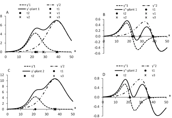
Figure 2 shows the graphs of the derivatives of the first and second orders, with the location of the abscissas of the inflection points for two plants. In the interval (-∞; ∞), in (B) the derivative of second order y” = y”1 + y”2 intercepts the x-axis three times, and in (D) just once. The x value that defines the interphase, 26.49 months in the model III, is quite close to the estimate of the abscissa of the intersection point between the two logistics in model II, 25.59 months. These are points that
Table 3 – Mean (standard deviation) of the x values that are roots of the second order derivative functions (abscissas of the inflection points) and fourth order (abscissas of the stability points) of models I - monophasic, II - diphasic segmented and III - diphasic sum. (n = number of trees).
Abscissas of inflection points Abscissas of stability points
Models (n) phase 1 inter-phases phase 2 phase 1 phase 2
Model I (29) .. .. 33.46(1.902) .. 48.36(2.088)
Model II (26) 22.07(2.104) .. 34.47(1.560) 29.07(3.583) 50.46(3.594)
Model III (26) 21.26(1.392) 26.49(2.295) 36.60(0.950) 27.16(2.314) 47.41(2.828)
[20.90(1.271)] .. [36.80(1.062)] [27.48(2.626)] [47.44(2.843)]
Figure 2 – Inflection points in the diphasic logistic sum in an example of two plants of Eucaliptus grandis. In (A) first order derivatives (y’) and in (B) second order (y”) for plant 1: a1 = 58.057, b1 = -6.506, c1 = 0.2898, a2 = 141.104, b2 = -7.632, c2 = 0.1959, t1 = 22.45, t2 = 38.95, v1 = 23.81, v2 = 28.61, v3 = 38.62; in (C) and (D) for plant 2: a1 = 52.603, b1 = -7.096, c1 = 0.3333, a2 = 222.031, b2 = -6.952, c2 = 0.1906, t1 = 21.29, t2 = 36.48, v = 36.28 months. The abscissas t1 and t2 are estimates of τ1 and τ2; v1, v2, v3, of υ1, υ2, υ3.
can define the separation between the two phases of growth of the organism.
In determining the points that are the roots of the fourth order derivative in model III, the diphasic sum, there were five solutions for (16), considering as stability points the third solution, xe1 = the abscissa of the stability point of y in phase 1, and the fifth solution xe2 = the abscissa of the stability point of y in growth phase 2. These solutions are different from those ob-tained when determining stability points considering a function for each phase. Table 3 presents the averages of the abscissas of the stability points: in model I they are the third solution of the equation y(4) = 0; in model
II, the third solution for phase 1 and the sixth for phase 2; in model III, the third solution for phase 1 and the fifth for phase 2.
The abscissas of the stability points in phase two of models II and III are quite similar to the values found for model I, for all plants. The abscissas determined by the logistics at each stage in model III (Table 3 in brack-ets) are very similar, but not identical to those that are the roots of the fourth order derivative of the sum func-tion; this can be observed in all plants.
Conclusions
The use of a diphasic logistic to represent eu-calyptus growth up to 50 months was more effective than a monophasic logistic. The critical points of in-flection and stability are determined in the diphasic segmented model by the known formulas for deter-mining these points in monophasic models, but in the diphasic model sum, the points that are the roots of second and fourth orders derivatives cannot be deter-mined explicitly, and their values are different from those determined for the individual logistics compo-nents of this model.
References
Beyene, S.; Ramakrishnan, V. 2013. A numerical method for estimating the variance of age at maximum growth rate in growth models. Communications in Statistics: Theory and Methods 42: 1464-1475.
Breusch, T.S.; Pagan, A.R. 1979. A simple test for heteroscedasticity and random coefficient variation. Econometrica 47: 1287-1294. Brody, S.; Ragsdale, A.C. 1921. The rate of growth of the dairy
cow. The Journal of General Physiology 3: 623-633.
Draper, N.R.; Smith, H. 1998. Applied Regression Analysis. 3ed. John Wiley, New York, NY, USA.
Fenner, T.; Levene, M.; Loizou, G. 2013. A bi-logistic growth model for conference registration with an early bird deadline. Central European Journal of Physics 11: 904-909.
Grossman, M.; Koops, W.J. 1988. Multiphasic analysis of growth curves in chickens. Poultry Science 67: 33-42.
Koops, W.J. 1986. Multiphasic growth analysis. Growth 50: 169-177.
Koops, W.J.; Grossman, M.; Michalska, E. 1987. Multiphasic growth curve analysis in mice. Growth 51: 372-382.
Koops, W.J.; Grossman, M. 1991. Applications of a multiphasic growth function to body composition in pigs. Journal of Animal Science 69: 3265-3273.
Kurnianto, E.; Shinjo, A.; Suga, D. 1999. Multiphasic analysis of growth curve body weight in mice. Asian-Australasian Journal of Animal Sciences 12: 331-335.
Mendes, P.N.; Muniz, J.A.; Silva, F.F.; Mazzini, A.R.A. 2008. Difasics logistic model in the study of the growth of Hereford breed females. Ciência Rural 38: 1984-1990 (in Portuguese, with abstract in English).
Mendes, P.N.; Muniz, J.A.; Silva, F.F.; Mazzini, A.R.A.; Silva, N.A.M. 2009. Analysis of the difasics growth curve of Hereford females by the Gompertz non-linear function. Ciência Animal Brasileira 10: 454-461 (in Portuguese, with abstract in English).
Mischan, M.M.; Pinho, S.Z.; Carvalho, L.R. 2011. Determination of a point sufficiently close to the asymptote in nonlinear growth functions. Scientia Agricola 68: 109-114.
Narinc, D.; Karaman, E.; Firat, M.Z.; Aksoy, T. 2010. Comparison of non-linear growth models to describe the growth in Japanese Quail. Journal of Animal and Veterinary Advances 9: 1961-1966.
Nešetřilová, H. 2005. Multiphasic growth models for cattle. Czech Journal of Animal Science 50: 347-354.
Özkan, M. 2004. Diphasic analysis of growth in Japanese quail. Asian-Australasian Journal of Animal Sciences 17: 1281-1285. Passos, J.R.S.; Pinho, S.Z.; Carvalho, L.R.; Mischan, M.M.
2012. Critical points in logistic growth curves and treatment comparisons. Scientia Agricola 69: 308-312.
Portz, L.; Dias, C.T.S.; Cyrino, J.E.P. 2000. A broken-line model to fit fish nutrition requirements. Scientia Agricola 57: 601-607. Robbins, K.R.; Saxton, A.M.; Southern, L.L. 2006. Estimation of
nutrient requirements using broken-line regression analysis. Journal of Animal Science 84: E155-E165.
Schinckel, A.P.; Craig, B.A. 2002. Evaluation of alternative nonlinear mixed effects models of swine growth. The Professional Animal Scientist 18: 219-226.
Seber, G.A.F.; Wild, C.J.1989. Nonlinear Regression. John Wiley, New York, NY, USA.