APPLICATION OF HYBRID AND POLYTOPIC MODELING TO THE
STABILITY ANALYSIS OF LINEAR SYSTEMS WITH SATURATING INPUTS
J.M. Gomes da Silva Jr
∗ [email protected]S. Tarbouriech
† [email protected]R. Reginatto
∗ [email protected]∗UFRGS - Departamento de Engenharia El´etrica, Av. Osvaldo Aranha 103, 90035-190 Porto Alegre-RS, Brazil.
†LAAS-CNRS, 7 Avenue du Colonel Roche, 31077 Toulouse cedex 4, France.
ABSTRACT
This paper is concerned with the problem of stability regions determination for linear systems with saturating inputs. The paper focuses on a critical analysis of two known approaches to model the effect of actuator saturation: hybrid modeling and polytopic modeling. In each case, algorithms to deter-mine ellipsoidal domains of stability for such class of sys-tems are provided in terms of LMIs. The ability of such algorithms in providing large stability domains is analyzed by highlighting the main reasons they incorporate conserva-tiveness, including the influence of the saturation modeling. Two examples are worked out illustrating how significantly the stability domains obtained by such algorithms can dif-fer.
KEYWORDS: Control saturation, hybrid modeling,
poly-topic modeling, stability analysis
RESUMO
Este artigo trata do problema de determinac¸˜ao de regi˜oes de estabilidade para sistemas lineares com entradas saturantes. O trabalho foca-se em uma an´alise cr´ıtica de duas abordagens conhecidas para o modelamento dos efeitos da saturac¸˜ao de controle: modelamento h´ıbrido e modelamento polit ´opico.
Artigo submetido em 5/12/2002
1a. Revis ˜ao em 4/08/2003; 2a. Revis ˜ao 19/03/2003
Aceito sob recomendac¸ ˜ao do Ed. Assoc. Prof. Jos ´e R. C. Piqueira
Em cada caso, algoritmos para determinar dom´ınios de es-tabilidade para a classe de sistemas considerada s˜ao pro-postos em termos de LMIs. A habilidade de tais algorit-mos em fornecer grandes dom´ınios de estabilidade ´e anali-sada, enfatizando-se as principais fontes de conservatismo, incluindo o pr´oprio modelamento da saturac¸˜ao. Dois exem-plos s˜ao apresentados a fim de ilustrar o qu˜ao diferente po-dem ser os dom´ınios de estabilidade obtidos com os diferen-tes algoritmos.
PALAVRAS-CHAVE: Saturac¸˜ao de controle, modelamento
h´ıbrido, modelamento polit ´opico, an´alise de estabilidade.
1
INTRODUCTION
Silva Jr. et al., 1997; Hu e Lin, 2000) which opens another approach, and a corresponding set of results, to deal with the stability analysis and synthesis problems.
One of the most concerning problems in this subject is the determination of asymptotic stability regions for the closed-loop system. The motivation for these studies is that, in the presence of control saturation, global stability cannot in general be ensured. Furthermore, when it is possible to compute a global stabilizing control law (see (Sussmann et al., 1994; Burgat e Tarbouriech, 1996)), in general it is difficult to simultaneously guarantee good performance and robustness for the closed-loop system. On the other hand, on the ground of local stabilization, the exact determination of the basin of attraction is possible only in very particular cases. Hence it is important to determine asymptotic stabil-ity regions, in order to approximate the basin of attraction (Khalil, 1992).
The proposed methods for generating stability regions for linear systems with saturating inputs explore the special structure of these systems and are mainly based on the concept of Lyapunov domains. Special classes of Lya-punov functions have been considered for such purpose, for instance, piecewise-linear (Gomes da Silva Jr. e Tar-bouriech, 1999b), quadratic (see, for example, (Henrion e Tarbouriech, 1999; Gomes da Silva Jr. e Tarbouriech, 1999c; Fong e Hsu, 2000; Hu e Lin, 2000) and references therein) and Lure type (Pittet et al., 1997; Hindi e Boyd, 1998) Lya-punov functions. In order to obtain testable results, the choice of each class of Lyapunov functions is connected to the choice of a convenient representation for the effect of the saturation function. Moreover, both the choice of the Lya-punov function and the saturation modeling are directly re-lated to the conservatism of the results.
In this paper we particularly focus on the hybrid and poly-topic representations for linear systems with input saturation and aim at determining ellipsoidal domains of stability. The interest for such domains is mainly motivated by the recent developments concerning numerical algorithms and software packages for solving LMIs and convex optimization prob-lems. This fact allows the implementation of test conditions that can be cast as LMI-based optimization problems where the optimization criteria can be related, directly or indirectly, to the size of the domain of stability to be computed.
Although these methods involve some degree of conser-vatism, in general the conservatism of the results is not conveniently analyzed or elucidated. It can be noticed a lack of critical comparison between the different approaches. Hence, one of the objectives of this paper is to provide a crit-ical analysis of some methods for computing ellipsoidal re-gions of asymptotic stability for systems with saturating
in-puts. In parallel, we briefly discuss how to use the proposed conditions for the synthesis of local stabilizing control laws. Additionally, we propose two new LMI stability conditions based on a hybrid representation of the saturated system and the use of the S-procedure.
The paper is organized as follows. Section 2 states the prob-lem, related concepts, and definitions. In Sections 3 and 4, two strategies to model the saturation effect are discussed, namely: the modeling by a hybrid system and the model-ing by a polytopic system. In each one of these sections the sufficient conditions to be satisfied and the corresponding al-gorithms for determining the ellipsoidal regions of stability are presented and discussed, including related synthesis is-sues. Finally two examples are worked out, in Section 5, in order to provide a numerical comparison between the results obtained with the different approaches. The paper is ended with concluding remarks in Section 6.
Notations. For any vector x ∈ ℜn, x 0 means that all the components ofx, denotedx(i), are nonnegative. For two
vectors x, y of ℜn, the notationx y means that x( i)− y(i)≥0,∀i = 1, . . . , n. A(i)denotes theith row of matrix A. For two symmetric matrices,A andB,A > Bmeans thatA−Bis positive definite. A′ denotes the transpose of A. diag(x)denotes a diagonal matrix obtained from vector
x. 1m △
= [1. . .1]′ ∈ ℜm, 0 m
△
= [0. . .0]′ ∈ ℜm andI denotes the identity matrix of appropriate dimensions.int S
denotes the interior of the setS.
2
PROBLEM STATEMENT
Consider the continuous-time linear system
˙
x(t) =Ax(t) +Bu(t) (1)
wherex(t)∈ ℜn,u(t)∈ ℜm,A∈ ℜn×nandB ∈ ℜn×m. Assume system (1) is in closed-loop with the saturated linear control law
u(t) =sat(Kx(t)) (2)
wheresat(·)denotes a classical saturation function, i.e. each component i (i = 1,· · ·, m) of vector u(t), is defined as follows:
u(i)(t) = (sat(Kx(t)))(i)
=
−ρ(i) ifK(i)x(t)<−ρ(i) K(i)x(t) if −ρ(i)≤K(i)x(t)≤ρ(i)
ρ(i) ifK(i)x(t)> ρ(i)
(3)
whereρ(i)and -ρ(i)represent the control limits.
Due to the saturation term, the closed-loop system is nonlin-ear:
˙
The polyhedral set
S(K, ρ)△=
x∈ ℜn;
K −K
x
ρ ρ
(5)
is the region of linearity of system (4). Inside this region, the control entries do not saturate and the behavior of the system is described by the linear model
˙
x(t) = (A+BK)x(t) (6)
Throughout the paper we assume that the matrixKis such that all the eigenvalues of(A+BK)are placed in the open left half complex plane. In other words, in the absence of control bounds, the closed-loop system would be globally asymptotically stable.
Consider now the ellipsoidal set
E(P, c) ={x∈ ℜn; x′P x≤c}
(7)
whereP =P′>0andc >0.
Definition 2.1 The setE(P, c)is aregion of asymptotic sta-bilityfor system (4) if:(i)the pointx= 0is a locally asymp-totically stable equilibrium point; (ii)it is contained in the region of attraction of the equilibriumx= 0.
Definition 2.2 The setE(P, c)iscontractivewith respect to system (4) if the functionV(x) =x′P xis strictly decreasing along the trajectories of (4) inE(P, c)− {0}. In particular, ifE(P, c)is contractive, then it is a region of asymptotic sta-bility.
In particular, the problem of determining ellipsoidal regions of stability contained in the regionS(K, ρ)is a trivial prob-lem (see (Boyd et al., 1994) for instance). In this paper, we are interested in the study of conditions that allow the de-termination of stability regions not contained in the region of linearity and, in consequence, that take into account the nonlinear characteristic of the closed-loop system.
3
HYBRID SYSTEM MODELING
Due to the specific structure of the saturation function (3), the system (4) naturally exhibits a hybrid structure. This representation consists in dividing the state space in regions calledregions of saturation. Inside each region of satura-tion, the system (4) can be modeled as an affine system or, equivalently, as a system with an additive constant distur-bance (Gomes da Silva Jr. e Tarbouriech, 1999b),(Gomes da Silva Jr. e Tarbouriech, 1999a). Thus, the saturated system (4) is viewed, generically, as a hybrid system whose dynam-ics is piecewise linear (Johansson e Rantzer, 1998).
Consider a vectorη(t) ∈ ℜm, such that each entryη
(i)(t), i= 1, . . . , m, takes the values1,0or−1in accordance with the saturation function (3) as follows:
η(i)(t) =
−1 ifK(i)x(t)<−ρ(i)
0 if −ρ(i)≤K(i)x(t)≤ρ(i)
1 ifK(i)x(t)> ρ(i)
(8)
Letξj ∈ ℜm,j = 0,1,· · ·,3m−1, represent all possible values ofη(t). Then,∀t,η(t) = ξj for somej and hence, each vectorξj represents a possible combination between saturated and non-saturated control entries. Furthermore, for
η(t) =ξj, the state vector belongs to a specific region called
region of saturationj. Each region of saturation is defined by the intersection of half-spaces of the formK(i)x≤ d(i)
or −K(i)x ≤ d(i), where d(i) can be eitherρ(i) or −ρ(i).
Generically, the region of saturation associated toξj is de-noted as:
S(Rj, dj) ={x∈ ℜn; Rjxdj} (9)
wheredj ∈ ℜlj is defined from the entries ofρand−ρ, and
Rj ∈ ℜlj×n is defined from the rows ofK and−K (see numerical examples of the regions description in (Gomes da Silva Jr. e Tarbouriech, 1999b) and (Gomes da Silva Jr. e Tarbouriech, 1999a)).
We defineξ0 = 0m and so the region associated toj = 0 corresponds toS(K, ρ). In the other regions there is at least one control entry that is saturated. Thus, the motion of the system (4) can be described by the following hybrid system
˙
x(t) = A¯jx(t) +vj, x(t)∈S(Rj, dj),
j= 0,1,· · ·,3m−1 (10)
withA¯j=A+Bdiag(1m− |ξj|)Kandvj =Bdiag(ξj)ρ, where|ξj|is taken componentwise.
Theorem 1 The functionV(x) =x′P x,P =P′ >0, is a
strictly decreasing Lyapunov function for the saturated sys-tem inE(P, c)if and only if the following conditions hold:
(i) x′P(A+BK)x+x′(A+BK)′P x <0, ∀x∈S(K, ρ)∩ E(P, c), x6= 0
(ii) x′P( ¯A
jx+vj) + ( ¯Ajx+vj)′P x <0,
∀x∈S(Rj, dj)∩ E(P, c),∀j, j= 1, . . . ,3m−1,
st S(Rj, dj)∩intE(P, c)6=∅
(11)
Although Theorem 1 provides a necessary and sufficient con-dition for a setE(P, c)to be contractive, it still lacks of prac-tical benefit because the conditions (11)-(i)(ii)are not easily solvable with the available numerical methods. In the se-quel we present two conditions that, despite being only suffi-cient for the satisfaction of (11)-(i)(ii), are numerically more tractable.
3.1
Test Condition 1
The condition below corresponds to a generalization, to multi-input systems, of the results proposed in (Fong e Hsu, 2000).
Proposition 1 If there exist a matrixP ∈ ℜn×n,P =P′ >
0, and nonnegative scalarsγjandτj(i), i= 1, . . . , lj satisfy-ing the followsatisfy-ing matrix inequalities
(i)P(A+BK) + (A+BK)′P <0
(ii)
PA¯j+ ¯A′jP−γjP P vj−0.5R′jTj′
v′
jP−0.5TjRj γjc+Tjdj
<0
∀j, j= 1, . . . ,3m−1,
such that S(Rj, dj)∩intE(P, c)6=∅
(12) withTj = [τj(1) . . . τj(lj)], then the setE(P, c)is a region
of asymptotic stability for the saturated system (4).
Proof:Relation (12)-(i)implies that relation (11)-(i)is sat-isfied for allx 6= 0. Ifx ∈ S(Rj, dj)∩intE(P, c)then
xsatisfies
x′P x−c≤0
Rjx−dj 0 . Hence, it follows that a suf-ficient condition for the satisfaction of (11)-(ii)is that for some nonnegative scalarsγjandτj(i), i= 1, . . . , ljone ver-ifies
x′(PA¯
j+ ¯A′jP)x+x′P vj+vj′P x−γj(x′P x−c)
− lj
X
i=1
τj(i)(Rj(i)x−dj(i))<0, ∀x, x6= 0 (13)
or, equivalently
x′ 1
G
x
1
<0 ∀x, x6= 0 (14)
with
G=△ "
PA¯j+ ¯A′jP−γjP P vj−0.5P lj
i=1τj(i)R′j(i)
vj′P−0.5
Plj
i=1τj(i)Rj(i) γjc+P lj
i=1τj(i)dj(i)
#
It follows that a sufficient condition for the satisfaction of (14), and, in consequence, for the satisfaction of (11)-(ii)is given by
PA¯j+ ¯A′jP−γjP P vj−0.5R′jTj′
v′
jP−0.5TjRj γjc+Tjdj
<0 (15)
which completes the proof. ✷
The result of Proposition 1 allows to verify whether a given ellipsoidal setE(P, c)is contractive or not. It also allows to compute an estimate of the region of attraction of the origin in two different ways:
(a) Given a contractive setE(P, c)one can try an homoth-etic expansion by interactively increasingcand testing the condition (15). In this case, the test corresponds to solve an LMI feasibility problem.
(b) Use condition (12) to directly find a contractive set E(P, c)for system (4). In this case, however, the condi-tion (12)-(ii)becomes a BMI sinceP andγj will both be decision variables. The solution of a BMI is much more complex than an LMI, and is usually performed by employing some relaxation method (Goh et al., 1996). It is important to remark that, sincePis a decision vari-able,ccan be taken as1without loss of generality. A possible relaxation algorithm is as follows.
Algorithm 3.1
1. Chooseγj=γ,∀j= 1, . . . ,3m−1.
2. Setc= 1. Fixγj,j= 1, . . . ,3m−1, obtained in the previous step and search forPandTjby opti-mizing a criterion on the size ofE(P, c)subject to the LMI conditions (12)1.
3. FixP obtained in step 2. Maximizec subject to conditions (12) withγjandTj,j= 1, . . . ,3m−1 as free variables2.
4. Go to step 2.
The steps 2 and 3 of the algorithm are performed it-eratively until a desired precision in the size criterion forE(P, c)is achieved. Note that,(P, γj, Tj)obtained in step 2 consists in a feasible solution for step 3 with
c = 1. Conversely,(P, c, γj, Tj)obtained in 3 is a fea-sible solution for step 2 by settingPasP/c. Hence the convergence of the algorithm is always ensured.
Remark 1 Computational burden can be reduced in the im-plementation of inequalities (12) by removing all regions of saturation that are symmetric with respect to the origin, since the satisfaction of (12) in one region of saturation also im-plies its satisfaction in the region symmetric to it.
1Sinceγjare given, the condition becomes an LMI.
2This can be accomplished by increasing interactivelycand testing (12)
Remark 2 The condition (11)-(ii)has been turned into con-dition (12)-(ii), which can be verified as an LMI test or, in the worse case, as a BMI. In this transformation, however, some conservatism has been introduced due to the following facts:
1. The determination of the stability conditions is based on the S-procedure (see inequality (13)). Indeed, the S-procedure is only a sufficient condition in this case because there is more than a single constraint involved (Boyd et al., 1994).
2. The LMI test (15) implies that
x′ z′ ˜
G
x z
<0 (16)
for all(x, z) 6= 0, while it would be enough to check the case wherez= 1.
3. The need of a relaxation method implies that we are not certain to find a solution of the problem even if it ex-ists. Moreover, whenever a solution is found, there is no guarantee that solution is the best that could have been found.
4. It is clear that the contractive setE(P, c)does not neces-sarily intersect all the regions of saturation. Moreover, only the region that do intersect the set need to be tested. However, if the setE(P, c)is being synthesized, it is not possible to determine, a priori, whether the searched el-lipsoid will intersect or not some of the regions of satu-ration. In this case, in Algorithm 3.1 the test of (12)-(ii)
is performed for all regions of saturation. Hence, it can happen that condition (12)-(ii)is unnecessarily verified in some regionj.
3.2
Test Condition 2
The condition below was mainly inspired by the results pre-sented in (Johansson e Rantzer, 1998) for generic hybrid sys-tems.
Proposition 2 If there exist a matrixP ∈ ℜn×n,P =P′ >
0, symmetric matricesMj ∈ ℜlj×lj with nonnegative en-tries, and nonnegative scalarsγjsatisfying the following ma-trix inequalities
(i) (A+BK)′P+P(A+BK)<0
(ii)
PA¯j+ ¯A′jP+R′jMjRj−γjP P vj−R′jMjdj
v′jP−d′jMjRj γjc+d′jMjdj
<0
∀j, j= 1, . . . ,3m
−1,
such that S(Rj, dj)∩ E(P, c)6=∅
(17)
then the setE(P, c)is a region of stability for the saturated system (4).
Proof:Relation (17)-(i)implies that relation (11)-(i)is sat-isfied.
Condition (11)-(ii)can be rewritten as:
[x′ 1]
P 0 0 0
¯
Aj vj
0 0
x
1
+[x′ 1]
¯ A′ j 0 v′ j 0 P 0 0 0 x 1
<0 (18)
∀j= 1, . . . ,3m−1,∀x such that
x′P x−c≤0 Rjx−dj0 .
Let nowMj ∈ ℜlj×lj be a symmetric matrix with nonneg-ative entries and letγj be a nonnegative scalar. It follows that
x′ 1
− R′ j d′ j Mj
−Rj dj
x
1
≥0,
∀x: Rjx−dj 0 (19)
γj[x′ 1]
−P 0
0 c x
1
≥0, ∀x: x′P x−c≤0 (20)
Using now the S-procedure, it follows that a sufficient con-dition for the concon-dition (11)-(ii)is that, for some symmetric matrixMj ∈ ℜlj×lj with nonnegative entries and a nonneg-ative scalarγj, one has,∀x6= 0,
x 1 ′ P 0 0 0 ¯
Aj vj
0 0 + ¯ A′ j 0
vj′ 0
P 0
0 0
+
−R′
j
d′j
Mj
−R′
j
d′j
′ +γj
−P 0
0 c x 1 <0 (21)
Hence, a sufficient condition for the satisfaction of (21), and, in consequence, for the satisfaction of (11)-(ii) is:
PA¯j+ ¯A′jP+R′jMjRj−γjP P vj−R′jMjdj
vj′P−d′jMjRj γjc+d′jMjdj
<0
(22)
which completes the proof. ✷
As it can be concluded from the proofs, Propositions 2 and 1 basically differ in the strategy the S-procedure is handled. In Proposition 2 the constraints are tranformed into quadratic forms (19), (20) before being included in the matrix inequal-ities. Due to the similarity in the development of the two propositions, all the remarks made about Proposition 1, con-cerning Algorithm 3.1 and Remarks 1 and 2, apply to Propo-sition 2.
Remark 3 In the single input case, sinceMj is a is a non-negative scalar it follows thatd′
for (19) which yields the following equation as a replacement for (21), x 1 ′ P 0 0 0 ¯
Aj vj
0 0
+
¯
A′j 0
v′ j 0 P 0 0 0 +
−R¯′j
¯ d′ j Mj
−R¯j d¯j
+γj
−P 0
0 c
x
1
<0
withR¯j =
Rj
0
andd¯j =
dj
1
. In this caseMj ∈
ℜ2×2and, sinced
jhas always at least one negative element,
¯
d′
jMjd¯j can assume negative values depending on the Mj entries.
3.3
Synthesis Issues
As seen in the previous section, the conditions stated in Propositions 1 and 2 can be directly applied to the problem of estimating the region of attraction of system (4). In this sec-tion we discuss how to use these condisec-tions for addressing the following synthesis problem.
Problem 1 Compute a matrixKsuch that the saturated state feedback control law defined by (3) ensures that for all initial states belonging to a given set of admissible initial condi-tionsX0, the corresponding trajectories of system (4)
con-verge asymptotically to the origin.
In order to address this problem, define diagonal matrices
Q1j,Q2jandΛjas follows
Q1j(i,i)=
−1 if ξj(i)= 1
0 if ξj(i)=−1
1 if ξj(i)= 0
i= 1, . . . , m (23)
Q2j(i,i)=
0 if ξj(i)= 1
1 if ξj(i)=−1 −1 if ξj(i)= 0
, i= 1, . . . , m (24)
Λj(i,i)= (1− |ξj(i)|), i= 1, . . . , m (25)
From the definitions (23)-(25), it follows that:
Rj=QjK △ = Q1j Q2j
K; dj = ˜Qjρ △
=
Q1j −Q2j
ρ
For the sake of simplicity, considerX0 as a polyhedral3 set
described by its vertices:
X0 △
=Co{v1, . . . , vn
v}, vs∈ ℜ
n ∀s= 1, . . . , n v (26)
Based on Proposition 1 the following synthesis result can be stablished.
3It could be also ellipsoidal or an union of ellipsoidal and polyhedral
sets.
Proposition 3 If there exist a matrixW =W′ > 0,W ∈ ℜn×na matrixY ∈ ℜm×n, matricesT
j∈ ℜ1×2mwith non-negative entries, and scalarsγj >0,c > 0andβ > 1such that the following matrix inequalities are satisfied:
(i) (AW +BY) + (AW+BY)′<0
(ii)
AW +W A′+BΛ
jY +Y′ΛjB′−γjW
v′
j−0.5TjQjY
vj−0.5Y′Q′jTj′
γjc+TjQ˜jρ
<0, ∀j, j= 1, . . . ,3m−1
(iii)
c βv′ s
βvs W
≥0 , ∀s= 1, . . . , nv
(27) then the gainK=Y W−1solves Problem 1.
Proof: Withβ >1condition(iii)ensures that the setX0is
contained in the ellipsoidal setE(P, c), withP =W−1. Pre
and post multiplying(i)and(ii) by the matrix
P 0 0 I
and consideringK =Y W−1, it follows, from the proof of
Proposition 1, thatE(P, c)is a contractive set for the system (4). Hence if x(0) ∈ X0, it follows thatx(0) ∈ E(P, c)
which ensures that the corresponding trajectory of system (4) converges asymptotically to the origin.✷
Considering W, Y, Tj, γ andc as decision variables, in-equalities (27)-(ii)in Proposition 3 are nonlinear and thus very hard to solve. On the other hand, if we fix some of these variables the conditions becomes LMIs. This is the case, for instance, if we fixγjandTj. Of course, for givenγjandTj it may actually be impossible to find a feasible solution for LMIs (27). In fact, considering a scaling factor β,β > 0, the maximum homothetic set toX0,βX0, that can be
stabi-lized considering the fixedγjandTj, can be obtained solving the following convex optimization problem with LMI con-straints:
max
β,c,W,Y β subject to
LMIs(i),(ii),(iii)of Proposition 3
(28)
Algorithm 3.2
1. Fixc= 1and solve (28) without constraints (27)-(ii).
2. FixY obtained in the previous step, gridγ (γ = γj, ∀j = 1, ...,3m−1) and findTj,W andcconsidering the maximization of the scaling factorβfor each value ofγin the grid. Take the solutionW, Tj, csuch thatβ is maximal.
3. FixγandTj, obtained in the previous step, and solve forW,Y andcconsidering as optimization criteria the maximization ofβ.
4. Go to step 2.
The algorithm stops when no significant improvement in the value ofβ is achieved or whenβ ≥1. For the same argu-ments given in Algorithm 3.1, the convergence of the algo-rithm is always ensured. In this case, if the final value ofβis greater than one, a solution to Problem 1 is given by the final values ofW andY.
As pointed out in the analysis case, a drawback of the pro-posed approach is that conditions (27)-(ii)should be verified in all regions of saturation. It is implicitly assumed that the regionX0will have a non empty intersection with all the
re-gions of saturation, which is not always true. However, since the definition of the regions of saturation depends on the ma-trixKto be computed, it is impossible to verify this a priori.
The development of synthesis results on the basis of Propo-sition 2 leads to the following inequality as a replacement for (27)-(ii):
A
jW +W A′j+Y′Q′jMjQjY −γjW
v′
j−ρ′Q˜′jMjQjY
vj−Y′Q′jMjQ˜j
γjc+ρ′Q˜′jMjQ˜jρ
<0
Due to the termsY′Q′
jMjQjY, this inequality is more dif-ficult to solve consideringY andMj as decision variables. One way to handle this problem would be to forceMj to be positive definite and apply Schur’s complement. However, note that this is impossible because, in this case, the term
γjc+ρ′Q˜′jMjQ˜jρwould be always positive. Hence, the ap-plication of the test condition 2 for the synthesis problem is not very interesting.
4
POLYTOPIC SYSTEM MODELING
Note that theith entry of the saturated control law defined in (3) can be also written as:
(sat(Kx(t)))(i)=α(x(t))(i)K(i)x(t) (29)
where0< α(x(t))(i)≤1, is defined as :
α(x(t))(i)=
−ρ(i)
K(i)x(t) ifK(i)x(t)<−ρ(i)
1 if −ρ(i)≤K(i)x(t)≤ρ(i)
ρ(i)
K(i)x(t) ifK(i)x(t)> ρ(i)
(30) The coefficientα(x(t))(i) can be viewed as an indicator of
the degree of saturation of theith entry of the control vector. In fact, the smaller theα(x(t))(i), the farther the state vector
is from the region of linearity (5). Notice thatα(x(t))(i)is a
function ofx(t).
Define from the vector α(x(t)) ∈ ℜm a diagonal matrix
D(α(x(t))) =△ diag(α(x(t))). Thus, system (4) can be rewritten as
˙
x(t) = (A+BD(α(x(t))K)x(t) (31)
Theorem 2 The functionV(x) =x′P x,P =P′ >0, is a
strictly decreasing Lyapunov function for the saturated sys-tem inE(P, c)if and only if the following condition hold:
x′[(A+BD(α(x))K)′P+P(A+BD(α(x))K)]x <0, ∀x∈ E(P, c), x6= 0
(32)
Proof:it follows directly from (31).✷
4.1
Approach 1
Let0< α(i) ≤1be a lower bound toα(x(t))(i)and define
the vectorα= [△ α(1), ..., α(m)]′. The vectorαis associated
to the following region in the state space:
S(K, ρα) ={x∈ ℜn;
K −K
x
ρα
ρα
} (33)
whereρα
(i) △
= ρ(i)
α(i),∀i= 1, . . . , m.
Consider now all the possiblem-order vectors such that the
ith entry takes the value1orα(i). Hence, there exists a
to-tal of2m different vectors. By denoting each one of these vectors byγj,j = 1, . . . ,2m, define the following matrices:
Dj(α) = D(γj) = diag(γj)andAj = A+BDj(α)K. Note that the matrices Aj are the vertices of a convex polytope of matrices. If x(t) ∈ S(K, ρα) it follows that
(A+BD(α(x(t)))K) ∈ Co{A1, A2, . . . , A2m}. Hence,
ifx(t)∈S(K, ρα),x˙(t)can be determined from an appro-priate convex linear combination of matricesAj at timet, that is:
˙
x(t) =
2m
X
j=1
λj(x(t))Ajx(t) (34)
withP2m
j=1λj(x(t)) = 1, λj(x(t))≥0.
It should be pointed out that model (34) represents the satu-rated system only inS(K, ρα). Actually, ifx(t)∈S(K, ρα), the polytopic model (34) can be used to determinex˙(t).
Proposition 4 If there exist a matrixP = P′ > 0, P ∈ ℜn×n, a vectorα∈ ℜmand a positive scalarcsatisfying the following conditions
(i) P(A+BDj(α)K) + (A+BDj(α)K)′P <0, ∀j= 1, . . . ,2m
(ii)
"
P α(i)K(′i) α(i)K(i) ρ2(i)/c
#
≥0 ∀i= 1, . . . , m
(iii) 0< α(i)≤1 ∀i= 1, . . . , m
(35) then the setE(P, c)is a region of stability for the saturated system (4).
Proof: Provided conditions(ii)and(iii)are verified it fol-lows thatE(P, c)is contained inS(K, ρα)(Gomes da Silva Jr. et al., 1997; Boyd et al., 1994).
Hence, for allx(t) ∈ E(P, c),∀t ≥ 0, it follows that there existsλj(x(t)), withP2
m
j=1λj(x(t)) = 1, λj(x(t)) ≥ 0,
such that:
˙
x(t) = (A+BD(α(x(t))K)x(t) =
2m
X
j=1
λj(x(t))Ajx(t)
(36) From condition(i)it follows that
x(t)′P 2m
X
j=1
λj(x(t))(A+BDj(α)K)x(t)
+
2m
X
j=1
x(t)′λj(x(t))(A+BDj(α)K)′P x(t)<0 (37)
or equivalently,
x(t)′(A+BD(α(x(t)))K)′P x(t)
+x(t)′P(A+BD(α(x(t)))K)x(t)<0 (38)
Since this reasoning is valid∀x(t)∈ E(P, c),x6= 0,∀t≥0, from Theorem 2 it follows thatE(P, c)is a region of stability for the saturated system.✷
Similarly to Propositions 1 and 2, the sufficient condition stated in Proposition 4 allows both to test if a givenE(P, c)is contractive and to determine a contractive set based on some geometric criterion:
• In the first case, since P and c are given, conditions (35)-(i)(ii)(iii)can be easily tested as an LMI feasibil-ity problem in variableα.
• In the second case, P andα appear as problem vari-ables4 and conditions (35)-(i) become BMIs whereas (35)-(ii)(iii)are LMIs. As pointed out in section 3.1, the presence of a BMI constraint makes difficult the di-rect solution of an optimization problem. A possible relaxation scheme in this case is as follows (see (Gomes da Silva Jr. e Tarbouriech, 1999c) and (Henrion e Tar-bouriech, 1999) for more details):
Algorithm 4.1
1. Chooseα.
2. Set c = 1. Fixαobtained in the previous step, search forP by optimizing a criterion on the size ofE(P, c)subject to the LMI constraints given by (35)-(i)(ii)
3. FixPobtained in step 2. Minimizeµ= 1c subject to LMI constraints given by (35)-(i)(ii)(iii)with
αas free variable.
4. Go to step 2.
The convergence of Algorithm 4.1 can be concluded by a reasoning similar to Algorithm 3.1.
Remark 4 The conservatism of the condition given by Proposition 4 is due to the modeling of the behavior of the saturated system by a differential inclusion. In fact, (35)-(i)is a necessary and sufficient condition for the quadratic stability of the polytopic system
˙
x(t) =
2m
X
j=1
λj(t)Ajx(t) (39)
∀λj(t)such thatP2
m
j=1λj(t) = 1, λj(t) ≥ 0. Note, however, that all trajectories of the saturated system (4) are also trajectories of system (39), but the converse is not necessarily true.
4.2
Approach 2
Consider a matrixH¯ ∈ ℜm×nand define
S( ¯H, ρ)△={x∈ ℜn;
¯
H
−H¯
x
ρ ρ
}
Let now matricesΘj,j = 1, . . . ,2mbe diagonal matrices whose diagonal elements are equal to 1 or 0. From these definitions, ifx(t)belongs to the setS( ¯H, ρ), it can be shown (by convexity arguments) thatx˙(t)can be computed by the following polytopic model:
˙
x(t) =
2m
X
j=1
λj(x(t))(A+B(ΘjK+ (I−Θj) ¯H)x(t) (40)
withP2m
j=1λj(x(t)) = 1, λj(x(t))≥0. Similar to the pre-vious section, the model (34) represents the saturated system only in the regionS( ¯H, ρ).
Proposition 5 (Hu e Lin, 2000) If there exist matricesP =
P′ >0,P ∈ ℜn×nandH ∈ ℜm×n, and a positive scalarc satisfying the following conditions
(i) P[A+B(ΘjK+ (I−Θj) ¯H)]
+[A+B(ΘjK+ (I−Θj) ¯H)]′P <0, ∀j= 1, . . . ,2m
(ii)
"
P H¯′ (i)
¯
H(i) ρ2(i)/c
#
≥0, ∀i= 1, . . . , m
(41)
then the setE(P, c)is a region of stability for the saturated system (4).
Proof:Considering that(ii)ensures thatE(P, c)⊂S( ¯H, ρ), the proof follows similarly to the one of Proposition 4.✷
By settingW = P−1,γ = 1
c one can state the following corollary.
Corollary 3 If there exist a symmetric positive definite ma-trixW, a positive scalar γ and a matrixGsatisfying the following LMIs:
(i) AW +B(ΘjKW+ (I−Θj)G) +W A′
+(ΘjKW + (I−Θj)G)′B′<0, ∀j= 1, . . . ,2m
(ii)
"
W G′ (i) G(i) γρ2(i)
#
≥0 ∀i= 1, . . . , m
(42)
thenH¯ = GW−1 and the setE(P, γ−1) ⊂ S( ¯H, ρ)is a region of stability for the saturated system (4).
Considering a criterion on the size of the regionE(P, γ−1),
the conditions given in Proposition 5 or in Corollary 3 can be straightforwardly applied to the determination of ellipsoidal regions of stability for the saturated system. The main ad-vantage of this approach is that the conditions are LMIs and no relaxation scheme is needed. Note that in this case we can considerγ= 1without loss of generality. Regarding the conservativity of the modeling, similar comments stated in Remark 4 apply to this approach.
4.3
Synthesis Issues
Following the same reasoning presented in section 3.3, the condition proposed in Proposition 4 can be used for synthesis purposes. This result is formalized as follows:
Proposition 6 (Gomes da Silva Jr. et al., 1997) If there exist matricesW =W′ >0,W ∈ ℜn×nandY ∈ ℜm×n and a vectorα∈ ℜm, satisfying the following matrix inequalities:
(i) W A′+AW +BD
j(α)Y +Y′Dj(α)B′<0 ∀j= 1, . . . ,2m
(ii)
W Y′
(i) Y(i) (ρ(i)/α(i))2
≥0 , ∀i= 1, . . . , m
(iii)
1 v′ s
vs W
≥0 , ∀s= 1, . . . , nv
(iv) 0< α(i)≤1, i= 1, . . . , m
(43) thenK=△Y W−1solves Problem 1.
As in the Proposition 3, inequalities (43)-(i) and (43)-(ii)
The same discussion done in the previous section is valid here. A similar iterative algorithm can be proposed in or-der to find a solution for Problem 1 consior-dering a given set X0 of admissible initial conditions (see (Gomes da Silva Jr
e Tarbouriech, 2001)). Note that here the algorithm will be simpler than the Algorithm proposed in section 3.3 since it suffices to iterate two steps: in the first step we fixαand in the second we fixY.
On the other hand, the result of Corollary 3 can be used for synthesis purposes by substituting (43)-(i)and (43)-(ii)by
(i) AW +B(ΘjY + (I−Θj)G) +W A′
+(ΘjY + (I−Θj)G)′B′<0, ∀j = 1, . . . ,2m
(ii)
"
W G′ (i) G(i) ρ2(i)
#
≥0 ∀i= 1, . . . , m
In this last case, as in the analysis case, the constraints appear directly as LMIs in the decision variablesW,Y andGwhich avoid the use of relaxation schemes.
5
NUMERICAL EXAMPLES
The algorithms to synthesize ellipsoidal stability domains for linear systems with saturation described in the paper will now be applied to two different systems. The goal is to compare the effectiveness of the algorithms in synthesizing large sta-bility domains and to verify the actual effect of the conserva-tive steps involved in each algorithm.
For each system we solve the problem of finding an ellip-soidal asymptotic stability domain by applying each of the methods described in the paper. For each method, we search for the best possible ellipsoid, in the attempt to finding the largest possible region of stability. All the results are plot-ted to allow a visual comparison of the size of the stability regions obtained with each method.
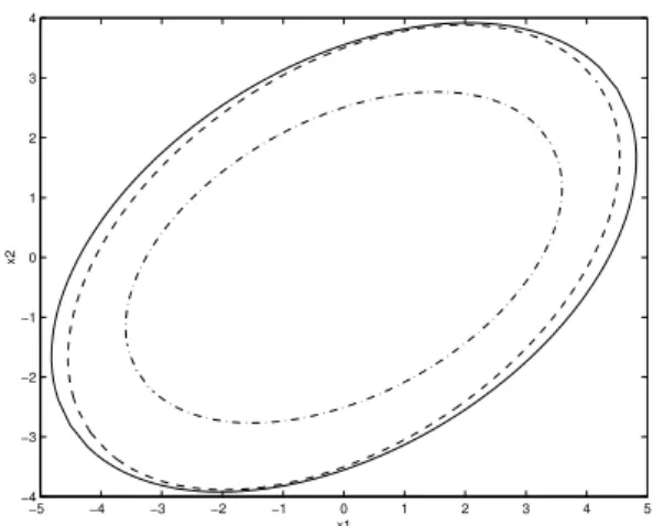
Example 5.1 We consider first a single input, second order linear system in closed-loop by a linear state feedback with saturation. The parameter of this system are:
A=
0.5 −1 1 0.5
; B=
0.5 1
;
K=
0.278 −2.139
; ρ= 4
• Result obtained with the hybrid modeling 1st condition:
The criterion considered was the maximization of the minor axis of the ellipsoidal region (i.e. minimization of the greater eigenvalue ofP). The optimal value of
−5 −4 −3 −2 −1 0 1 2 3 4 5
−4 −3 −2 −1 0 1 2 3 4
x1
x2
Figure 1: hybrid modeling 1st and 2nd condition (dash-dotted); polytopic 1st approach (dashed); polytopic 2nd ap-proach (solid)
this criterion is obtained forγ= 2.1with
P =
0.0942 −0.0517
−0.0517 0.1591
; c= 1
• Result obtained with the hybrid modeling 2nd condi-tion:
The optimal value of this criterion is obtained forγ = 2.1with
P =
0.0942 −0.0517
−0.0517 0.1591
; c= 1
• Result obtained with the polytopic modeling 1st ap-proach:
Applying the Algorithm 4.1, considering in step 2 the minimization of the greater eigenvalue ofPand starting withα= 1we obtain
P =
0.0596 −0.0302
−0.0302 0.0816
; c= 1
• Result obtained with the polytopic modeling 2nd ap-proach:
One obtains:
P =
0.0525 −0.0273
−0.0273 0.0793
; c= 1
Figure 1 depicts the ellipsoids obtained with the different ap-proaches.
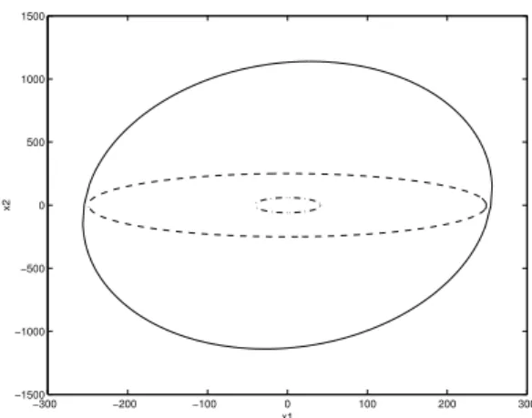
Example 5.2 Consider now the following multi-input sec-ond order linear system with:
A=
0.1 −0.1 0.1 −3
; B=
5 0 0 1
;
K=
−0.7283 −0.0338
−0.0135 −1.3583
; ρ=
5 2
• Result obtained with the hybrid modeling 1st condition:
Applying the Algorithm 3.1, considering as criterion the maximization of the minor axis of the ellipsoidal region (i.e. minimization of the greater eigenvalue ofP), the best value forγin the first step is0.25. With this value one obtains
P = 10−3
0.5886 0.0023 0.0023 0.2800
; c= 1
• No solution was found with the hybrid modeling 2nd condition.
• Result obtained with the 1st polytopic modeling ap-proach:
Applying the Algorithm 4.1, considering also the maxi-mization of the minor axis of the ellipsoidal region and initializingαas1m, we obtain
P = 10−4 0.1608 0.0001
0.0001 0.1592
; c= 1
withα=
0.0275 0.0034 ′ .
• Result obtained with the 2nd polytopic modeling ap-proach:
P = 10−4
0.1542 −0.0038
−0.0038 0.0078
; c= 1
Figure 2 depicts the ellipsoids obtained with the different ap-proaches.
Note that the set obtained with the hybrid modeling 1st con-dition is significantly smaller than the set obtained with the polytopic approaches. Moreover the 2nd polytopic approach gives a less conservative domain than the 1st one.
6
CONCLUDING REMARKS
We have considered the local stability and stabilization prob-lems for saturated linear systems in a comparative study con-text. We focused on the determination of ellipsoidal do-mains of stability by employing quadratic Lyapunov func-tions. This has been done for two different approaches to
−300 −200 −100 0 100 200 300
−1500 −1000 −500 0 500 1000 1500
x1
x2
Figure 2: hybrid modeling 1st condition (dash-dotted); poly-topic 1st approach (dashed); polypoly-topic 2nd approach (solid)
model the saturated system: a hybrid modeling and a poly-topic modeling. Based on the results presented and the sim-ulations provided, it is possible to draw de following conclu-sions:
• Two main sources of conservativeness can be identified: the modeling and the strategy to develop a testable con-dition. It is clear that these two aspects are connected, since the modeling determines, in a large extent, the tools that can be applied to obtain testable conditions.
• The main source of conservativeness in the hybrid mod-eling case comes from the transformation of the prob-lem into a set of matrix inequalities, which requires the use of the S-procedure among other key assumptions.
• The main source of conservativeness in the polytopic modeling can be identified as the abstraction of the modeling. The test condition considersλj as arbitrary functions of time that live between given limits, thus ne-glecting their intrinsic link to the state.
As far as the computational burden is concerned, the two test conditions derived from the hybrid modeling are similar. In this case, a set of3mLMIs have to be solved. On the other hand, the polytopic modeling involves2mLMIs, thus being less computationally expensive.
REFERENCES
Boyd, S., El Ghaoui, L., Feron, E. e Balakrishnan, V. (1994).
Linear Matrix Inequalities in System and Control The-ory, SIAM Studies in Applied Mathematics.
Burgat, C. e Tarbouriech, S. (1996). Stability and control of saturated linear systems,inA. Fossard e D. Normand-Cyrot (eds),Non-Linear Systems, Vol. 2, Chapman & Hall.
Fong, I.-K. e Hsu, C.-C. (2000). State feedback stabilization of single input systems through actuators with satura-tion and deadzone characteristics, Proc. of 39st IEEE Conference on Decision and Control (CDC’00), Syd-ney, Australia.
Goh, K., Safonov, M. G. e Ly, J. H. (1996). Robust synthesis via bilinear matrix inequalities, Int. J. of Robust and Nonlinear Control6: 1079–1095.
Gomes da Silva Jr., J. M., Fischman, A., Tarbouriech, S., Dion, J. M. e Dugard, L. (1997). Synthesis od state feedback for linear systems subject to control satura-tion by an lmi-based approach,Proc. of the 2nd IFAC Workshop on Robust Control Design (ROCOND’97), Budapest, Hungary, pp. 229–234.
Gomes da Silva Jr., J. M. e Tarbouriech, S. (1999a). Invari-ance and contractivity of polyhedra for continuous-time linear systems with saturated controls,Revista Controle e Automac¸˜ao da SBA10(3): 149–158.
Gomes da Silva Jr., J. M. e Tarbouriech, S. (1999b). Polyhe-dral regions of local asymptotic stability for discrete-time linear sytems with saturating controls, IEEE-Trans. on Automatic Control44: 2081–2086.
Gomes da Silva Jr., J. M. e Tarbouriech, S. (1999c). Stabil-ity regions for linear systems with saturating controls,
Proc. of the European Control Conference (ECC’99), Karlsrhue, Germany.
Gomes da Silva Jr, J. M. e Tarbouriech, S. (2001). Local stabilization of discrete-time linear systems with satu-rating controls: an LMI-based approach,IEEE-Trans. on Automatic Control46: 119–125.
Henrion, D. e Tarbouriech, S. (1999). LMI relaxations for ro-bust stability of linear systems with saturating controls,
Automatica35: 1599–1604.
Hindi, H. e Boyd, S. (1998). Analysis of linear systems with saturation using convex optimization, Proc. of 37th IEEE Conference on Decision and Control (CDC’98), Tampa, USA, pp. 903–908.
Hu, T. e Lin, Z. (2000). An analysis and design method for linear systems subject to actuator saturation and dis-turbance, Proc. of the American Control Conference (ACC’00), Chicago, USA.
Johansson, M. e Rantzer, A. (1998). Computation of piece-wise quadratic lyapunov functions for hybrid systems,
IEEE-Trans. on Automatic Control43(4): 555–559.
Khalil, H. K. (1992). Nonlinear Systems, MacMillan.
Molchanov, A. e Pyatnitskii, E. (1989). Criteria of asymp-totic stability of differential and difference inclusions encountered in control theory,Systems&Control Let-ters13: 59–64.
Pittet, C., Tarbouriech, S. e Burgat, C. (1997). Stability re-gions for linear systems with saturating controls via cir-cle and popov criteria,Proc. of 36th IEEE Conference on Decision and Control (CDC’97), San Diego, USA, pp. 4518–4523.
Sussmann, H., Sontag, E. e Yang, Y. (1994). A gen-eral result on the stabilization of linear systems using bounded controls, IEEE-Trans. on Automatic Control