Design Considerations on a Dispersion
Compensating Coaxial Fiber
F.D. Nunes
Departamento de Eletr^onica e Sistemas, Centro de Tecnologia, Universidade Federal de Pernambuco,
Caixa Postal 7800, 50711-970 Recife, PE, Brazil
H. F.da Silvaand S. C.Zilio
Instituto de Fsica de S~ao Carlos, Universidade de S~ao Paulo, Caixa Postal 369, 13560-970 S~ao Carlos, SP, Brazil
Received September 30, 1997
This work reports the performance of a dispersion compensating coaxial ber as a function of its geometric parameters. Our analysis is carried out by solving the wave equation under the linearly polarized approximation, which leads to transcendental equations that provide the eective index of refraction. The highest eciency at a xed wavelength is achieved for a suitably chosen geometry and this choice is an important factor to determine the general shape of the wavelength-dependent dispersion curve.
I. Intro duction
The development of Erbium-doped ber ampliers with gain at 1.55 m suggests the need of upgrading the existing 1.31m optical ber links for operation in that wavelength. This will bring the advantage of using unrepeted long-haul systems. However, transmission of high data rates over long distances using the already installed single mode bers (SMF) requires the use of techniques to compensate the pulse spreading caused by positive chromatic dispersion. In order to accomplish this goal, many researchers have directed their atten-tion to the use of dispersion compensating bers (DCF) [1-4]. Peschel et al. [3] have recently shown that the su-permodes of two dissimilar coupled planar waveguides may exhibit dispersion compensation and discussed the trade-o between group velocity dispersion (GVD) and bandwidth. Their theoretical analysis was carried out with the coupled wave guides model, where the modes in each isolated sub-structure are coupled through a coupling constant . Based on the idea of dissimilar waveguides, Thyagarajan et al. [4] extended this con-cept to a cylindrical geometry by performing a
wavelength), is obtained as well as universal dispersion curves for any ber mode.
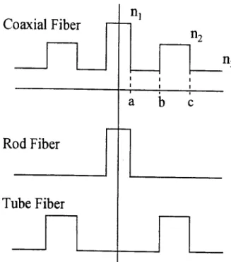
Figure 1. Refractive index radial prole of the dispersion compensating coaxial ber. The sub-structures that com-pose the coaxial ber (rod and tube) are also shown.
The present work employs the theoretical frame-work developed in ref. [9] to determine the dispersion coecient of coaxial bers, by performing a numerical calculation of the second order derivative ofn. There-fore, the procedure adopted here is dierent from that using coupled modes [3], and also from the numerical approach developed in ref. [7]. The emphasis in this work is placed on the dependence of the dispersion co-ecient on the geometrical parameters, namely, the rod radius,a, the outer gap radius,b, and the outer barrier radius,c. When they change, the depth and bandwidth of the wavelength-dependent dispersion coecient can change signicantly. There is a trade-o between the group velocity dispersion and bandwidth [3], and then it becomes important to determine the shape of the wavelength-dependent dispersion coecient for dier-ent design situations.
II. Fiber design and theoretical framework
As mentioned in the previous section, the disper-sion coecient is calculated through the second deriva-tive of the eecderiva-tive refracderiva-tive index curve. These curves
are obtained with the LP approximation for the coax-ial ber that has the prole shown in Fig. 1, and the resulting transcendental equations are those presented for the W1 structure (with n
2 = n
4) in ref. [9]. The values of the refractive indicesn
1and n
2are calculated by adding to the lower refractive index value, n
3, the same steps employed in ref. [4], namely , 1 = 0
:02 and 2 = 0
:003; where i = (
n 2 i ,n 2 3)
=(2n 2 3)
: The wavelength dependence is assumed to be the same for all refractive indices. n
3 was calculated with the well-known Sellmeier equation: [10]
n 2 3= 1 +
3 X j=1 A j 2 j ( 2 , 2 j) (1) with A
1 = 0
:69681388; A 2 = 0
:40865177; A 3 = 0:89374039;
1 = 0
:070555513; 2 = 0
:11765660 and
3= 9
:8754801[10]. Assuming the same parameters for all refractive indices does not aects the general trend of the results presented here, but a better approach is being searched for future work. Unfortunately, up to the author's knowledge, there are no available data to compare with the refractive index steps used here.
The dispersion coecient is calculated according to [11]:
D=, c d 2 n d 2 (2)
where cis the speed of light in vacuum. Once nis ob-tained from the transcendental equations,D() can be found by numerically determining its second derivative. The results were obtained with a Pentium 133 MHz , 32 Mb RAM personal computer, with the need of less than ve minutes to generate each data le forD. The mode proles can also be found with the theoretical approach given here, by substituting the propagation constant into the wave equation of the bers.
III. Numerical results and discussions
will present a positive dispersion. When any geomet-ric parameter changes, the wavelength where the phase matching occurs also changes, in addition to the shape of the dispersion curve. We rst discuss the inuence of the rod radius and of the outer gap radius in the disper-sion curve, for a given value of the outer barrier radius. With the theoretical approach described previously [9], we found to be possible to obtain pairs of geometric parameters (a;b) such that the dispersion occurs at the same wavelength, but the shape of the dispersion curve will depend on these parameters. This aects the de-sired compensation and constitutes the interest of the present work.
Figure 2. Indices of the supermodes HE11 and HE12 as a
function of the wavelength.
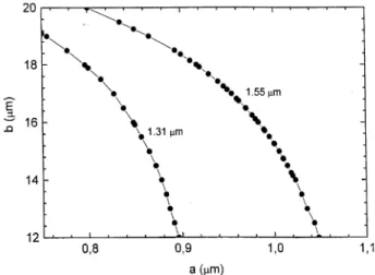
Fig. 3 shows the dependence of b on a such that the pairs (a;b) will result in \maximum dispersion" at the wavelengths of interest for communication systems, 1.31m and 1.55 m. The value ofcis kept constant at 22 m. The results indicate that any increase in the value of the rod radius can be compensated with a smaller value of the external gap region, as a way to produce the group velocity dispersion at the same wave-length. However, the behavior of the dispersion curve is much more sensitive to a than to b, meaning that a small variation in a requires a much larger change in b, as can be seen in Fig. 3. We have also calcu-lated wavelength-dependent dispersion curves for those pairs (a;b) shown as solid circles in Fig. 3 and the re-sults are presented in Fig. 4. The values of D found with the present theoretical approach are in good agree-ment with those of Thyagarajan et al. [4] for 1.55m when the same values of the ber parameters are used (a = 1:0 m , b = 15:2 m, c = 22 m, 1 = 0:02 and 2 = 0:003). The maximum dispersion occurs at a= 1:01m andb= 14:7m for 1.55m, anda= 0:87
m andb= 15m for 1.31m. Their values were found to beD1
:55
max=,4100 ps/(nm.km) andD1 :31
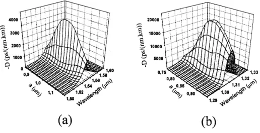
max=,21500 ps/(nm.km). Any increase or decrease of a results in a less ecient dispersion. Taking into account that the spectral half-width of a 10 ps pulse is about 3:510
,4 m, Fig. 4 indicates that the bandwidth of the coaxial DCF is suciently large for the two wavelengths con-sidered.
Figure 3. Pairs of geometric parametersa and bthat
pro-vides the maximum dispersion at wavelengths of interest for communication systems, 1.31m and 1.55m. The curves
are just for a visual aid.
Figure 4. Wavelength-dependent dispersion curves for dierent pairs (a;b) at (a) 1.55m and (b) 1.31m.
Figure 5. Pairs of radiusaandbthat provides the maximum
dispersion at 1.55m for dierent values ofc. The nearly
vertical curve corresponds to pairs that give the highest dis-persion.
Another point to be considered is the spatial eld distribution of the supermodes HE11 and HE12. They have modal proles with a central peak, which are quite similar for both modes and two lateral peaks, also sim-ilar in prole but with opposite signals. As already dis-cussed by Boucouvalas [8], these two supermodes are able to describe the fundamental modes of rod bers as well of tube bers, by either adding or subtracting them. When the modes HE11 and HE12are added, the lateral peaks cancel and the nal result is a Gaussian-like distribution as is the case of the fundamental mode of a rod ber. By taking their dierence, the central peaks will be canceled while the lateral peaks will be added, resulting in the prole of the fundamental mode of a tube [8]. Accordingly, it is possible to devise a way
to excite the fundamentalmode of the coaxial ber from the fundamental mode of a standard SMF with a taper made with a coaxial ber. When the SMF fundamental mode is launched into the taper, will be decoupled in two or more modes, in response to the lack of longi-tudinal invariance. In the case of an adiabatic taper, only the modes HE11 and HE12 will be excited, but just a small power (less then 10%) will be located in the HE12 mode and the remaining will be transported by the HE11 mode [12]. Therefore, there will a disper-sion compensation for most of the signal propagating in the coaxial ber. Since the mode HE12 has a positive dispersion it will be spreaded giving rise to a negligibly small pedestal. When the light reaches the end of the coaxial ber, another taper of appropriate length, will cause the opposite eect regenerating the fundamental mode of the SMF rod ber.
IV. Conclusions
were found to be in agreement with those of Thyagara-jan et al. [4]. The modal eld distribution for HE11and HE12were calculated, although not presented here, and the mechanism of excitation of the coaxial ber funda-mental mode from the fundafunda-mental mode of a rod SMF with a taper was discussed.
Acknowledgments
This work was supported by Fundac~ao de Amparo a Pesquisa do Estado de S~ao Paulo (FAPESP), Con-selho Nacional de Desenvolvimento Cientco e Tec-nologico (CNPq)/RHAE and program PRONEX, un-der the grant 4.1.96.0935.00.
References
[1] H. Izadpanah, C. Lin, J. L. Gimlett, A. J. Antos, D. W. Hall and D. K. Smith, Electron. Lett.28, 1469 (1992).
[2] A. J. Antos, and D. K. Smith, J. Lightwave Technol.
12, 1739 (1994).
[3] U. Peschel, T. Peschel, and F. Lederer, Appl. Phys. Lett.67, 2111 (1995).
[4] K. Thyagarajan, R. K. Varshney, P. Palai, A. K. Ghatak and I. C. Goyal, IEEE Photon. Technol. Lett.
8, 1510 (1996).
[5] K. C. Kao, and G. A. Hockham, Proc. IEE.113, 1151
(1966).
[6] M. M. Z. Kharadly, and J. E. Lewis, Proc. Inst. Elec. Eng.116, 214 (1969).
[7] E. Sharma, A. Sharma, and I. C. Goyal, IEEE J. Quant. Elect. QE-18, 1484 (1982).
[8] A. C. Boucouvalas, J. Lightwave Technol. LT-3, 1151
(1985).
[9] F. D. Nunes, C. A. de S. Melo, and H. Filomeno da Silva Filho, Appl. Optics35, 388 (1996).
[10] M. J. Adams,An Introduction to Optical Waveguides, John Wiley & Sons, pp. 213 (1981).
[11] D. Marcuse,Light Transmission Optics, Princeton, NJ: Van Nostrand, pp. 484, (1972).