Constrained Tensor Modeling Approach to
Blind Multiple-Antenna CDMA Schemes
Andr´e L. F. de Almeida, G´erard Favier, and Jo˜ao C. M. Mota
Abstract
In this paper, we consider an uplink multiple-antenna Code-Division Multiple-Access (CDMA) system linking several multiple-antenna mobile users to one multiple-antenna base-station. For this system, a constrained third-order tensor decomposition is introduced for modeling the multiple-antenna transmitter as well as the received signal. The constrained structure of the proposed tensor decomposition is characterized by two constraint matrices that have a meaningful physical interpretation in our context. They can be viewed as canonical allocation matrices that define the allocation of users’ data streams and spreading codes to the transmit antennas. The distinguishing features of the proposed tensor modeling with respect to the already existing tensor-based CDMA models are: i) it copes with multiple transmit antennas and spreading codes per user and ii) it models several spatial spreading/multiplexing schemes with multiple spreading codes by controlling the constrained structure of the tensor signal model. A systematic design procedure for the canonical allocation matrices leading to a unique blind symbol (or joint blind symbol-code) recovery is proposed which allows us to derive a finite set of multiple-antenna schemes for a fixed number of transmit antennas. Identifiability of the proposed tensor model is discussed, and a blind multiuser detection receiver based on the alternating least squares algorithm is considered for performance evaluation of several multiple-antenna CDMA schemes derived from the constrained modeling approach.
Index Terms
Blind detection, canonical allocation, CDMA systems, constrained tensor modeling, multiple-antenna schemes, spatial spreading, spatial multiplexing.
I. INTRODUCTION
It is well known that the use of multiple antennas at both the transmitter and receiver is promising since it potentially provides increased spectral efficiencies compared to traditional systems employing multiple antennas at the receiver only [1]. In the context of current and upcoming wireless communication standards, the integration of multiple-antenna and code-division multiple access (CDMA) technologies has been the subject of several studies [2]. Spatial multiplexing strategies in conjunction with CDMA is addressed in a few recent works [3]–[5] with focus on layered space-time processing. In [3], the multiple transmit antennas are organized in groups and a unique spreading code is allocated within the same group. The separation of the different groups at the receiver is done by using a layered spacetime algorithm [6]. Focusing on the downlink reception, [4] also considers the spatial reuse of the spreading codes and proposes a chip-level equalizer at the receiver to handle the loss of code orthogonality. A space-time receiver for block-spread multiple-antenna CDMA is proposed in [5]. In this case, block-despreading is used prior to space-time filtering in order to eliminate multi-user interference and reduce receiver complexity. On the other hand, CDMA-based transmit diversity schemes have been proposed earlier in [7], [8] and recently in [9]. These methods, commonly called space-time spreading, are capable of providing maximum transmit diversity gain without using extra spreading codes and without an increased transmit power. However, space-time spreading methods put more emphasis on diversity than on multiple-access interference. A recent work [10] investigates the performance of a range of linear single-user and multiuser detectors for multiple-antenna CDMA schemes with space-time spreading. In practice, due to the joint presence of multiple-access interference and time-dispersive multipath propagation, the large number of parameters to be estimated at the receiver (e.g. users’ multipath channels, received powers, spreading codes) may require too much processing/training overhead and degrade receiver performance. In a seminal paper [11], the problem of uplink multiuser detection/separation is linked to a Parallel Factor (PARAFAC) tensor model. It is shown that each received signal sample associated with a receive antenna, a symbol and a chip, can be interpreted as an element of a three-way array, or third-order tensor. Using this interpretation, [11] shows that the use of tensor modeling allows the receiver to
single-antenna transmissions.
The use of tensor decompositions for modeling multiple-antenna transmissions is proposed in [17]– [20]. A multi-antenna scheme based on a tensor modeling is proposed in [17]. Despite its diversity-rate flexibility and built-in identifiability, this multiple-antenna scheme relies only on temporal spreading of the data streams (as in a conventional CDMA system). Since there is no spatial spreading of the data streams across the transmit antennas, no transmit spatial diversity is obtained. In [18], a generalized tensor model is proposed for multiple-antenna CDMA systems with blind detection. However, this modeling approach only considers spatial multiplexing. In summary, the common characteristic of the tensor modeling approaches of [17] and [18] is that the number of data streams are restricted to be equal to the number of transmit antennas. The approach of [19] adds some flexibility at the transmitter by allowing the number of data streams to be different from the number of transmit antennas. As opposed to [17] and [18], full spatial spreading of each data stream across the transmit antennas is also permitted. It is shown that the corresponding tensor model has a fixed constrained structure that uniquely depends on the number of data streams and transmit antennas.
This paper presents a new modeling approach for uplink multiple-antenna CDMA schemes with blind multiuser detection. A constrained third-order tensor decomposition is introduced as a mathematical tool for modeling multiple-antenna CDMA schemes with multiple spreading codes. We show that several multiple-antenna schemes ranging from full transmit diversity to full spatial multiplexing and using different patterns of spatial reuse of the spreading codes can be modeled with the aid of two constraint matrices formed by canonical vectors. Physically, these matrices act as canonical allocation matrices
defining the allocation of users’ data streams and spreading codes to their transmit antennas. The distinguishing features of the proposed tensor model with respect to the existing tensor-based CDMA models can be briefly summarized as follows:
• The constraints in the tensor model allow to cope with multiple transmit antennas and spreading
codes per user or per data-stream, which provides an extension of [17]–[19] where each data stream is associated with only one spreading code;
• Several multiple-antenna schemes with varying degree of spatial spreading, spatial multiplexing and
spreading code reuse can be obtained by adjusting the constraint matrices of the tensor signal model accordingly.
schemes with a fixed number of transmit antennas. Identifiability of the proposed tensor model is discussed, and a blind joint detection receiver based on the alternating least squares algorithm is considered for performance evaluation of several multiple-antenna CDMA schemes.
It is worth mentioning that constrained tensor models has been an active research topic in other disciplines such as chemometrics [21]–[23]. Most of these works adopt a different interpretation of the constrained structure, by considering Tucker models [24] with constrained core tensor. Uniqueness is generally studied directly from the pattern of zeros of the core tensor. The “PARALIND” model, recently proposed for data analysis in the context of chemometrics problems [25], is probably the most related to our tensor model. This model also makes use of constraint matrices to model the dependence between columns of component matrices.
This paper is organized as follows. After presenting the basic notations used in this work, Section II defines the constrained tensor decomposition. Section III describes the basic system model. The proposed multiple-antenna CDMA model is presented in Section IV and linked to the constrained tensor decomposition. In Section V, the structure of the canonical allocation matrices of the tensor model is detailed and a design procedure for these matrices leading to a unique blind symbol recovery is described. In Section VI, some identifiability issues of the proposed model are discussed, and a blind receiver using an alternating least squares algorithm is proposed. Simulation results are presented in Section VII and the paper is concluded in Section VIII.
Notations: Scalar variables are denoted by lower-case letters (a, b, . . . , α, β, . . .), vectors are written as
boldface lower-case letters(a,b, . . . ,α,β, . . .), matrices correspond to boldface capitals(A,B, . . .), and
tensors are written as calligraphic letters (A,B, . . .). AT,A−1 and A† stand for transpose, inverse and
pseudo-inverse ofA, respectively. A−T denotes the inverse of the transpose ofA. The operator diag(a)
forms a diagonal matrix from its vector argument; blockdiag(A1, . . . ,AN)forms a block-diagonal matrix
withN matrix blocks;Di(A)forms a diagonal matrix holding thei-th row ofAon its main diagonal, i.e.,
Di(A) =diag(Ai·). The Kronecker and the Khatri-Rao products are denoted by ⊗and ⋄, respectively:
A⋄B = [A·1⊗B·1, . . . ,A·R⊗B·R]
=
BD1(A)
.. .
BDI(A)
∈C
IJ×R (1)
II. CONSTRAINED TENSOR DECOMPOSITION
In this section, we formulate a constrained tensor decomposition [14] which serves as the basic modeling tool for the considered multiple-antenna CDMA system. The link between this decomposition and the physical parameters of our system model is established in Section IV.
Definition: Let us consider a third-order tensor X ∈ CN1×N2×N3, three component matrices A(1) ∈ CN1×L1, A(2) ∈CN2×L2, A(3)∈CN3×F, and two constraint matrices Ψ∈CL1×F andΦ∈CL2×F. A
constrained tensor decomposition ofX with F component combinations is defined in scalar form as:
xn1,n2,n3 = F
X
f=1
L1
X
l1=1 L2
X
l2=1
a(1)n1,l1a(2)n2,l2a(3)n3,fψl1,fφl2,f,
with F ≥max(L1, L2), (2)
where xn1,n2,n3 is an entry of X ∈ C
N1×N2×N3, a(1) n1,l1 = [
A(1)]n1,l1, a(2)
n2,l2 = [
A(2)]n2,l2, a(3)
n3,f =
[A(3)]n3,f, are the entries of the first-mode, second-mode, and third-mode component matrices,
respec-tively. Similarly, ψl1,f = [Ψ]l1,f and φl2,f = [Φ]l2,f are, respectively, the entries of the two constraint
matrices. The columns ofΨandΦare canonical vectors1of canonical bases E(L1)
={e(L1)
1 , . . . ,e (L1)
L1 } ∈
RL1 and E(L2)
={e(L2)
1 , . . . ,e (L2)
L2 } ∈
RL2, respectively. The two constraint matrices define the component
combination pattern in the composition of the tensor. Otherwise stated, Ψ determines the coupling
between the columns of A(1) andA(3) whileΦ determines the coupling between the columns of A(2)
and A(3). It is assumed that Ψ and Φ are both full rank matrices, i.e. rank(Ψ)=L1 and rank(Φ)=L2.
Note that these assumptions mean that every canonical vector of the basis E(L1)
(resp. E(L2)
) appears at least once as a column ofΨ(resp.Φ). We defineαl1 ∈[1, F)as the number of component combinations
involving the l1-th column ofA(1), i.e., the number of times that the l1-th column of A(1) contributes
in the composition of the tensor X. Similarly, βl2 ∈ [1, F) is the number of component combinations
involving the l2-th column of A(2). αl1 (resp. βl2) corresponds to the number of 1’s entries at the l1-th
(resp. l2-th) row of Ψ(resp. Φ). We have:
ΨΨT = diag(α1, . . . , αL1) =diag(α),
ΦΦT = diag(β1, . . . , βL
2) =diag(β), (3)
1A canonical vectore(N)
whereα= [α1, . . . , αL1]andβ= [β1, . . . , βL2]are the component combination vectors of matricesA
(1)
andA(2), respectively. These vectors satisfy the following constraint:
L1
X
l1=1
αl1 = L2
X
l2=1
βl2 =F. (4)
As will be shown later, (2) is useful for modeling multiple-antenna CDMA systems with multiple spreading codes and data streams per user.
III. SYSTEM MODEL AND ASSUMPTIONS
We consider the uplink of a single cell synchronous multiple-antenna CDMA system with Q active users and spreading factor P. The base-station receiver is equipped with K antennas and the q-th user transmitsRqindependent data streams usingMqantennas. Multiple spreading codes per user are allowed,
andJqdenotes the number of spreading codes associated with theq-th user. Each transmitted data stream
containsN symbols. The wireless channel is assumed to be constant duringN symbol periods. Flat-fading and user-wise independent multipath propagation is considered. The transmit parameter set{Rq, Mq, Jq},
q= 1, . . . , Q, utilized by theq-th user, as well as the numberQof active users are assumed to be known
to the station receiver. Users’ spreading codes are symbol-periodic. We either assume that the base-station has perfect knowledge or has no knowledge of these spreading codes. The “unknown” spreading code assumption is valid in scenarii where multipath propagation induces Inter-Chip Interference (ICI). In this case, the term “spreading code” corresponds to the effective spreading code resulting from the convolution of the transmitted spreading code with the multipath channel [26]. We simply adopt the term “spreading code” throughout the paper for simplicity reasons. We distinguish three different types of multiple-antenna CDMA schemes covered by our modeling approach:
• Full spatial multiplexing: 1 < Rq = Jq = Mq. Each data stream is transmitted using a different
transmit antenna and a different spreading code (full code multiplexing).
• Full spatial spreading:1 =Rq≤Jq≤Mq. A single data stream is fully spread over all the transmit
antennas to achieve spatial transmit diversity. In this case, the number of used spreading codes may vary from one (full code reuse) up toMq (full code multiplexing).
• Combined spreading and multiplexing:1< Rq ≤Jq≤Mq. Each data stream is spread only across
We are mostly interested in combined spreading and multiplexing transmit schemes, since full mul-tiplexing and spreading can be considered as particular cases of the combined one. The constrained tensor modeling approach covers a wide variety of combined transmit schemes depending on the chosen constrained structure of the model. This is a key feature of our modeling approach as will be clarified later.
IV. TENSOR SIGNAL MODEL
For the multiple-antenna CDMA system described in the previous section, we formulate a new tensor model for the received signal, based on the constrained tensor decomposition defined in Section II. We start with a single-user model for simplicity reasons. Lethk,m be the spatial fading channel gain between the
m-th transmit antenna and thek-th receive antenna,sn,r =. s((r−1)N+n)be then-th symbol of ther-th
data stream, andcp,j be thep-th element of thej-th spreading code. Let us defineH∈CK×M,S∈CN×R
and C ∈ CP×J as the channel, symbol and code matrices, where hk,m = [. H]k,m, sn,r = [. S]n,r, and
cp,j = [. C]p,j are, respectively, the entries of these matrices. We can view the discrete-time baseband
version of the noise-free received signal at the n-th symbol period, p-th chip, and k-th receive antenna as a third-order tensorX ∈CN×P×K with the (n, p, k)-th element defined asxn,p,k=. xk((n−1)P+p). We propose the following input-output model for the considered multiple-antenna CDMA system:
xn,p,k= M
X
m=1
un,p,mhk,m, (5)
where un,p,m =. um((n−1)P +p) is the (n, p, m)-th element of the third-order tensor U ∈CN×P×M
representing the effective (precoded) transmitted signal. We treatU as the output of a constrained space-time spreading operation, which is modeled by the following constrained tensorial transformation:
un,p,m=
R
X
r=1
J
X
j=1
gm(r, j)sn,rcp,j, (6)
where
gm(r, j)=. ψr,mφj,m, (7)
is the (r, j)-th element of Gm ∈ CR×J. This matrix defines the allocation of R data streams and J spreading codes to them-th transmit antenna. Let us define:
G=ΨΦT ∈CR×J
respectively. The use of the terminology “canonical allocation” for ΨandΦis due to the fact that both
matrices are composed of canonical vectors controlling the coupling of R data streams andJ spreading codes to M transmit antennas, respectively.Ψcan be viewed as the stream-to-antenna allocation matrix
andΦ as the code-to-antenna allocation matrix.
The physical interpretation of (6) is that each data symbol sn,r is spread up to J times using the
spreading codes cp,1, . . . , cp,J. Each spread symbol sn,rcp,j is then loaded at the m-th transmit antenna.
Depending on the structure of the gm(r, j)’s, the same spread symbol sn,rcp,j may simultaneously be
loaded at several transmit antennas in order to benefit from transmit spatial diversity. From (5) and (6), we can express the received signal as
xn,p,k= M X m=1 R X r=1 J X j=1
gm(r, j)sn,rcp,jhk,m (8)
By comparing (2) and (8), we can deduce the following correspondences:
(N1, N2, N3, L1, L2, F) → (N, P, K, R, J, M),
(A(1),A(2),A(3)) → (S,C,H). (9)
A. Multiuser signal model
Some definitions are now introduced, which allow us to view (8) also as a multiuser signal model. In the multiuser case,R=R1+· · ·+RQ,J =J1+· · ·+JQ, andM =M1+· · ·+MQ denote, respectively,
the total number of data streams, spreading codes and transmit antennas considered, i.e., summed over all theQusers. In this case,H,SandCare interpreted as aggregate channel, symbol and code matrices
concatenating Q matrix-blocks, i.e.:
H = [H(1), . . . ,H(Q)]∈CK×M,
S = [S(1), . . . ,S(Q)]∈CN×R,
C = [C(1), . . . ,C(Q)]∈CP×J, (10)
where h(k,mq)
q
. = [H]
k,q− 1 P
i=1 Mi+mq
, s(n,rq)q
. = [S]
n,q− 1 P
i=1 Ri+rq
, and c(p,jq)
q
. = [C]
p,q− 1 P
i=1 Ji+jq
define the entries of the
q-th user channel, symbol and code matrices, respectively. We can also view the aggregate canonical
allocation matrices as a block-diagonal concatenation ofQ matrix-blocks:
Ψ = blockdiag(Ψ(1), . . . ,Ψ(Q))∈CR×M
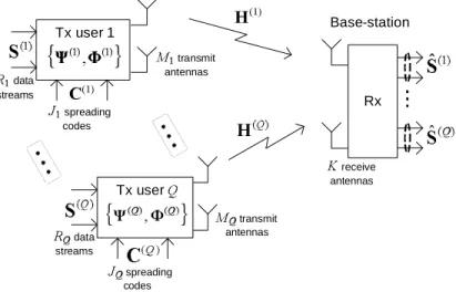
✁✂ ✄ ☎ ✆ ✝ ✞ ✟ ✠✡ ☛
Tx user 1
☞ ✌ data streams ✍ ✌ spreading codes ✎✑✏ transmit antennas ✎✑✒ transmit antennas ✓ ✒ data streams ✔ ✒ spreading codes Rx ✕ receive antennas ✖ ✗ ✘ ✙ ✚ ✛✜ ✢
{
✥✧✦✤✣ ★ ✥✤✣}
✩Tx user ✪
{
✬✮✭✰✯✯✲✱✫ ✬ ✫}
✳ ✴ ✵ ✶ ✷ Base-station ✸ ✹ ✺ ✻ ✼ ✽ ✾ ✿ ❀ ✷ ❁Fig. 1. Uplink model of the proposed multiple-antenna CDMA system.
where ψr(qq),mq
.
= [Ψ(q)]r
q,mq
. = [Ψ]q
−1
P
i=1 Ri+rq,
qP−1
i=1 Mi+mq
and φ(jqq),mq = [. Φ(q)]j
q,mq = [Φ]qP−1
i=1 Ji+jq,
qP−1
i=1 Mi+mq
define the entries of theq-th user allocation matrices. Similarly, the aggregate coupling matrix is defined as:
G = blockdiag(G(1), . . . ,G(Q)) =ΨΦT ∈CR×J,
with G(q)=Ψ(q)Φ(q)T, q= 1, . . . , Q. (12)
Figure 1 depicts the proposed multiple-antenna CDMA model.
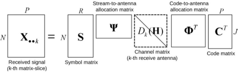
B. Matrix representations
The received signal model (8) can alternatively be expressed in equivalent matrix forms. Let us define
X··k ∈ CN×P collecting the P chips of the N transmitted symbols associated with the k-th receive
antenna. X··k can be factored in terms ofH, S, C, ΨandΦ as [15]:
X··k=SΨDk(H)ΦTCT, k= 1, . . . , K. (13)
We can also define two other matricesXn··∈CP×K collecting the received signal samples overP chips and K receive antennas associated with the n-th transmitted symbol, and X·p· ∈ CK×N collecting the received signal samples overN symbol periods andK receive antennas associated with thep-th chip of the spreading code. These matrices can be respectively factored as
Xn·· = CΦDn(SΨ)HT, (14)
=
✁ ✂
• •
✄
☎
✆
✝
✞ ✟
✠
✡
☛✌☞
✍
✎
Received signal (k-th matrix-slice)
Symbol matrix
Stream-to-antenna allocation matrix
Code-to-antenna allocation matrix
Code matrix Channel matrix
(k-th receive antenna)
✁
✏
✑
✒
Fig. 2. Constrained decomposition of the received signal tensor (k-th matrix slice of the third-mode).
and we have[Xn··]p,k= [X·p·]k,n = [X··k]n,p=xn,p,k. Using the tensorial terminology,{Xn··} ∈CP×K,
{X·p·} ∈ CK×N, and {X
··k} ∈ CN×P are called the first-, second- and third-mode matrix-slices,
obtained by “slicing” the tensor X ∈CN×P×K along its first, second, and third dimensions, respectively
[27]. Figure 2 illustrates the decomposition of X··k as a function of the aggregate symbol/code/channel
matrices{S,C,H}and the canonical allocation matrices{Ψ,Φ}. Let us define the three matricesX1=
[XT··1, . . . ,XT··
K]T ∈ CKN×P, X2 = [XT·1·, . . . ,XT·P·]T ∈ CP K×N, and X3 = [XT1··, . . . ,XTN··]T ∈
CN P×K concatenating the third-mode, second-mode and first-mode slices of the received signal tensor,
respectively, so that [X1](k−1)N+n,p = [X2](p−1)K+k,n = [X3](n−1)P+p,k = xn,p,k. These matrices are
usually called the “unfolded” representations of the signal tensor [27]. Using relation (1), we get [15]:
X1 =¡H⋄(SΨ)¢(CΦ)T, X2=¡(CΦ)⋄H¢(SΨ)T,
X3 =¡(SΨ)⋄(CΦ)¢HT. (16)
Relation to the PARAFAC model of [11]: The parallel can be made by assuming {Rq} = {Jq} =
{Mq} = 1. In this case, the correspondences between both tensor signal models are (M, R, J) →
(Q, Q, Q), and we have Ψ =Φ = IQ, meaning that the noiseless received signal model reduces to a
single-antenna CDMA tensor model [11]:
xn,p,k= Q
X
q=1
sn,qcp,qhk,q. (17)
Therefore, the proposed model can be viewed as a generalization of the one in [11], which is restricted to the single-antenna CDMA case. The introduction of Ψand Φ gives flexibility (and more degrees of
Remark 1: This constrained tensor model has properties similar to those of the tensor model proposed
in [12] for blind single-antenna CDMA systems with large delay spread. This model can be also viewed as a constrained tensor model where the constrained structure is fixed and intrinsic to the propagation channel (and not to the multiple-antenna transmitter design as in our context).
Illustrative example: In order to illustrate the physical meaning of the canonical allocation matrices,
let us consider the simple example of a single-user multiple-antenna system (Q= 1). Assume that the serial input stream is divided into R = 2parallel data streams transmitted by M = 4 transmit antennas usingJ = 3 orthogonal spreading codes. Suppose that the canonical allocation scheme is defined by the following constraint matrices:
Ψ=
1 1 0 0
0 0 1 1
, Φ=
1 1 0 0
0 0 1 0
0 0 0 1
(18)
The unitary entries in the first row of the stream-to-antenna allocation matrixΨmeans that the first data
stream is spread across the first and second transmit antennas. Likewise, the second row of Ψ shows
that the second data stream is spread across the third and fourth transmit antennas. Now, looking at the code-to-antenna matrix Φ, we can see that the first two antennas share the same spreading code
for transmission while the third and fourth transmit antennas are associated with different spreading codes. Several canonical allocation structures with different allocation patterns involving data streams and spreading codes for an arbitrary number of transmit antennas can be accommodated in our tensor model. However, the question is whether or not the chosen structure guarantees the uniqueness of the parameters of interest which are the symbol matrix and, possibly, the code matrix. In the next section, the design of the allocation matrices is studied.
V. DESIGN OF THE CANONICAL ALLOCATION MATRICES
In this section, we study the design of the canonical allocation matrices for ensuring blind symbol recovery (i.e. uniqueness ofS). The construction of the canonical allocation matrices satisfying a proposed
design criterion is presented. Then, we describe a procedure for designingΨ andΦwhich allows us to
derive a family of multiple-antenna schemes for a fixed number of transmit antennas.
A. Generating vectors
the same for all the users, we can bypass the user-dependent notation without loss of generality while simplifying the notation.
We propose to parameterize the two canonical allocation matrices by their generating vectors. Let us define α = [α1, . . . , αR] and β= [β1, . . . ,βR], where βr = [βr,1, . . . , βr,Jr], as the generating vectors
ofΨandΦ, respectively. These vectors completely characterize the canonical allocation structure in the
considered multiple-antenna system. Note that:
• αr is ther-th spatial spreading factor, and denotes the number of transmit antennas associated with
ther-th data stream;
• βr,jr is the jr-th code reuse factor, and denotes the number of transmit antennas using the jr-th
spreading code of ther-th data stream, jr= 1, . . . , Jr.
The generating vectorsα and β correspond to those defined in (3) for the constrained tensor decompo-sition. By analogy with (4), we have the following correspondences(l1, l2)→(r, j), (L1, L2)→(R, J)
andF →M, yielding the following constraint:
R
X
r=1
αr = R
X
r=1
Jr
X
jr=1
βr,jr =M. (19)
i.e. the sum of the elements of α= [α1, . . . , αR] is equal to that of β= [β1, . . . ,βR]which is always
equal to the number of transmit antennas.
B. Design criterion
We borrow some basic concepts from partition theory [28] in order to design the canonical allocation matrices. Specifically, the generating vectors α and β are interpreted here as partitions of size M and dimensions R and J, respectively. The fact that α and β are partitions of the same size is due to (19). Physically, α is a partition of M transmit antennas into R subsets transmitting different data streams (i.e.,ther-th data stream is spread acrossαr antennas). Likewise,β is a partition ofM transmit antennas
intoJ subsets, each one of which is associated with a different code (i.e., the j-th code is reused by βj
antennas). We suppose thatα and β satisfy the following design criterion:
Jr
X
jr=1
βr,jr =kβrk1=αr, 1≤r≤R, (20)
where Jr is the dimension of ther-th subpartitionβr = [βr,1, . . . , βr,Jr]of β, with J1+· · ·+JR=J.
βr,jr corresponds to the number of times the jr-th spreading code is reused within ther-th antenna set,
Based on (20), we propose the following partitioned construction for ΨandΦ:
Ψ = [Ψ1, . . . ,Ψr, . . . ,ΨR],
with Ψr=1T
αr ⊗e
(R)
r ∈RR×αr, r= 1, . . . , R,
(21)
and
Φ = [Φ1, . . . ,Φr, . . . ,ΦR],
with Φr= [Φr,1, . . . ,Φr,j
r, . . . ,Φr,Jr]∈R J×αr,
and Φr,j
r =
0
Jr−1×βr,jr
1T
βr,jr⊗e
(Jr) jr
0
(J−Jr)×βr,jr
∈R
R×βr,jr (22)
where 1n = [1,1, . . . , 1]T is an n-dimensional vector of ones, and Jr =
r
P
i=1
Ji. Note that Ψr is the
canonical allocation matrix associated with the r-th transmitted data stream, and Φr,j
r is the canonical
allocation matrix associated with thejr-th spreading code used by ther-th data stream.
Practical implications of the proposed design criterion: The proposed design criterion for determining
the structure of Ψ and Φ from α and β, respectively, has some practical implications. First, we can
observe that the spatial spreading of the data streams and the reuse of the spreading codes are restricted to adjacent transmit antennas only. This restriction can easily be deduced from the repetition pattern of identical canonical vectors in these matrices. Another implication of this construction is that different data streams cannot be associated with the same spreading code for transmission. In other words, spreading code reuse only takes place across the transmit antennas transmitting the same data stream.
ConstructingΨ(α)andΦ(β)according to the design criterion (20), we can verify (see the Appendix)
that any S˜ andC˜ satisfying the model are related toS and C, respectively, by:
˜
S = ST, T=diag(t1, . . . , tR)ΠR,
˜
C = CU, U=blockdiag(U1, . . . ,UR)ΠJ, (23)
where Ur ∈CJr×Jr is a non-singular transformation ambiguity matrix, Π
R ∈RR×R is a permutation
matrix and ΠJ ∈RJ×J is a block-diagonal permutation matrix. In other words, the symbol matrixS is
unique up to column permutation and scaling while the code matrixCis unique up to a multiplication by
uniqueness of S and C up to permutation and scaling arises in a particular case of (20) whereR =J
andαr=βr, r= 1, . . . , R.
Remark 2: The uniqueness of S is the major concern in this work, since our final goal is the blind
recovery of the transmitted data streams. On the other hand, the uniqueness ofH is not required, since
we are interested in a “direct” detection without using any knowledge about the channel.
C. Design procedure
We propose a systematic procedure for building the canonical allocation matricesΨandΦin (21)-(22)
based only on the generating vectorsα andβ, according to the following steps:
(i) A choice ofαis made for a fixed numberM of transmit antennas (partition size) and a fixed number R of input data streams (partition dimension);
(ii) For every αr, a sub-partition βr = [βr,1, . . . , βr,Jr]of size αr and dimension Jr is formed so that
(20) is satisfied and β= [β1, . . . ,βR]. The value ofJr, i.e. the number of spreading codes for the
r-th data stream, is a design parameter.
(iii) ΨandΦ are built according to (21)-(22).
D. Set of canonical allocation schemes
More than one choice forβmay be possible for a fixedα. This is due to the fact that more than one way of choosing a sub-partitionβr from αr, r= 1. . . , R may be possible without affecting the uniqueness
property of the model. Each choice will lead to a different allocation structure G = Ψ(α)Φ(β)T.
Following the proposed design procedure, a family of multiple-antenna CDMA schemes can be derived from the different possible choices of α and β. Table I shows the set of schemes for M = 4 transmit antennas. We assume that α1 ≥ · · · ≥ αR, and β1,1 ≥ · · · ≥ β1,J1 ≥ · · · ≥ βR,1 ≥ · · · ≥ βR,JR. This
assumption eliminates equivalent (redundant) schemes. For example, an allocation scheme withα= [1 3] andβ= [1 2 1]is considered equivalent to the one with α= [3 1] andβ= [2 1 1]. Both schemes have the same spreading and multiplexing pattern (the order of association of data streams and spreading codes with the transmit antennas is irrelevant), and have the same uniqueness property (both schemes satisfy (20)). In this table, the different schemes are listed according to increasing values ofR and J.
It can be seen from this table that 14 allocation schemes are possible. Note that for some values ofR andJ, 2 schemes exist. Let us consider the case(R, J) = (1,2), where we have 2 possible choices. For
TABLE I
FAMILY OF SCHEMES FORM = 4.
(R, J) α’s β’s nb. of schemes
(1, 1) 4 4 1
(1, 2) 4 {[3 1]; [2 2]} 2
(1, 3) 4 [2 1 1] 1
(1, 4) 4 [1 1 1 1] 1
(2, 2) {[3 1]; [2 2]} {[3 1]; [2 2]} 2 (2, 3) {[3 1]; [2 2]} [2 1 1] 2 (2, 4) {[3 1]; [2 2]} [1 1 1 1] 2 (3, 3) [2 1 1] [2 1 1] 1 (3, 4) [2 1 1] [1 1 1 1] 1 (4, 4) [1 1 1 1] [1 1 1 1] 1
antenna 4. On the other hand, for β= [2 2] each spreading code is used twice by two different antenna sets. Both are full spatial spreading schemes, but having different code reuse patterns. For(R, J) = (2,2), we have 2 feasible schemes, and they correspond to those satisfying α = β. For (R, J) = (2,3) and (2,4)we also have 2 schemes. Note that the basic difference between the schemes(R, J) = (2,2),(2,3)
and(2,4) is on the code reuse/multiplexing pattern, the spatial spreading pattern being the same.
E. Discussion
In practice, ΨandΦ can be designed based on practical restrictions such as the number of available
spreading codes and transmit antennas, data-rate and diversity requirements. One way of optimizing the allocation matrices is to take advantage of a priori channel state information at the transmitter. Since our design procedure allows the determination of a finite-set, or codebook, of feasible allocation schemes, limited feedback precoding methods [29], [30] can be used to select the best pair of constraint matrices at the transmitter. Although interesting, performance-oriented optimization ofΨandΦis a topic beyond
VI. BLIND RECEIVER
As far as multiuser separation/detection is concerned, the goal of the base-station receiver is to separate the Qusers’ transmissions (symbols/channels/codes) while recovering the data transmitted by each user. In this work, we consider a joint blind processing without using training sequences or resorting to a priori channel knowledge. In this case, model identifiability is a fundamental issue to be considered. This
issue is now studied.
A. Identifiability
Let us rewrite the three unfolded matrices of the received signal (16) in the following equivalent manner:
X1 = Z1¡H,S¢CT,
X2 = Z2¡C,H¢ST, (24)
X3 = Z3¡S,C¢HT,
where
Z1¡H,S¢ = ¡H⋄(SΨ)¢ΦT ∈CKN×J,
Z2¡C,H¢ = ¡(CΦ)⋄H¢ΨT ∈CP K×R,
Z3¡S,C¢ = (SΨ)⋄(CΦ)∈CN P×M, (25)
are the three constrained Khatri-Rao factorizations of the received signal model.
Theorem (identifiability): The identifiability of the constrained tensor model (8) in the Least Square
(LS) sense requires thatZ1¡H,S¢, Z2¡C,H¢, and Z3¡S,C¢ are full column-rank, which implies:
KN ≥J, P K≥R, and N P ≥M. (26)
Proof : The proof follows the same reasoning as the one given in [31] for the PARAFAC model. From
(24), C is identifiable in the LS sense if and only if Z1¡H,S¢ admits a unique left pseudo-inverse,
i.e. if it does not exist X 6= 0J belonging to the kernel K(Z1) such that Z1(X+CT) = Z1CT, i.e.
K(Z1) ={0J}. From the rank theorem, we have:
dim¡K(Z1)¢= 0⇒rank(Z1) =J,
which means that Z1 is full column-rank. Moreover, as we have rank(Z1) ≤ min(KN, J), it follows
From (26), the following corollaries can be obtained:
1) For R = J = M (equal number of data streams, spreading codes and transmit antennas), the constrained tensor decomposition reduces to the PARAFAC decomposition ofM factors, and (26) is equivalent to condition [31]:
min(N P, KN, P K)≥M
2) For 1< R =J < M (equal number of data streams and spreading codes) we can decouple (26) into the two following conditions:
K·min(N, P)≥R, and N P ≥M.
3) For 1< R < J=M (equal number of spreading codes and transmit antennas), we obtain the two following conditions:
N·min(K, P)≥M, and KP ≥R.
B. Discussion on the identifiability conditions:
1) Interpretation of (26): These identifiability conditions relate all the system parameters of interest,
which belong either to the transmitted or to the received signal dimensions. The transmitted signal dimensions are (R, J, M) while the receiver dimensions are (N, P, K). These conditions can be interpreted in the following manner. An increase in a transmitted signal dimension (e.g. data stream, spreading code, or transmit antenna dimension), representing an increase in the number of system
parameters to be identified at the receiver, must be compensated by an increase in the corresponding received signal dimension(s). As a consequence of tensor modeling, an identifiability tradeoff arises in (26). For instance, an increase in the number R of data streams can be compensated by increasing the numberKof receive antennas or the spreading factorP, or both, accordingly. A similar reasoning applies when the number of spreading codes or transmit antennas is increased.
2) k-rank based conditions: Model (16) can be viewed as a third-order PARAFAC model with three
equivalent factor matricesS=SΨ,C=CΦandH. Due to the presence of sets of identical columns in ΨandΦ, and consequently inSandC, the identifiability result of [11], which is based on the concept of
k-rank, does not apply to this constrained tensor model. This is due to the fact thatSandChavek-rank
C. Receiver algorithm
Now, we present the proposed blind receiver algorithm for symbol recovery. In order to exploit the tensor modeling of the received signal, we make use of the alternating least squares (ALS) algorithm [11], [21], which is the classical solution for estimating the component matrices of a tensor model. The ALS algorithm consists in fitting a third-order tensor model to the received data by alternatively minimizing three LS criteria. In our case, the component matrices to be estimated are the symbol, code and channel matrices, while the received data correspond to the noisy signal measured with the receiver antennas.
The ALS algorithm makes use of the three unfolded matrices representing the received signal in (24). We assume that the identifiability conditions (26) are fulfilled. At each step of this algorithm, one component matrix is estimated in the LS sense, while the two others are fixed to their values obtained at the two previous steps.ΨandΦare known matrices and are fixed during the iterative estimation process.
At the first iteration, Sb(0) and Hb(0) are randomly initialized. Assuming unknown spreading codes, the
ALS algorithm is composed of three estimation steps.
Define X˜i =Xi+Vi, i= 1,2,3, as a noisy version ofXi, whereVi is an additive complex-valued
white gaussian noise matrix.
1) Seti= 0;
Randomly initialize Hb(i=0) andSb(i=0);
2) i=i+ 1;
3) Using X˜1, find a LS estimate of C(i):
b
CT (i)=
h
Z1¡Hb(i−1),Sb(i−1)¢i†X˜1;
4) Using X˜2, find a LS estimate of S(i):
b
ST (i) =
h
Z2¡Cb(i),Hb(i−1)¢i†X˜2;
5) Using X˜3, find a LS estimate of H(i):
b
HT (i)=
h
Z3¡Sb(i),Cb(i)¢i†X˜3;
6) Repeat steps 2-5 until convergence.
of this algorithm can sometimes fall in regions of “swamps” during which the convergence speed is very small and the error between two consecutive iterations does not significantly decrease [21].
A more efficient initialization strategy consists in first obtaining an estimation of the column space of C, S and H using successive singular value decompositions of X1 ∈ CKN×P, X
2 ∈ CP K×N and X3 ∈ CN P×K, respectively. The estimated matrices are linked to the true ones by singular
non-admissible transformation matrices. They can, however, be used as a starting point of the ALS algorithm. This initialization procedure will probably be more efficient than a random initialization. Convergence of the estimates is rapidly achieved when the spreading code matrix C is known at the receiver [17].
In this case, the first estimation step is skipped. Assuming known spreading codes, we have observed that the ALS algorithm usually converges to the global minimum within 15-30 iterations for a SNR of 20 dB. In contrast, when considering unknown spreading codes, the convergence can be much slower. It can take hundreds or even thousands of iterations in worst-case situations.
Provided that condition (20) is satisfied, the ALS algorithm will provide a unique estimation of the symbol matrix Sb up to column permutation and scaling ambiguities. In order to eliminate the
scaling ambiguity, we assume that the first transmitted symbol of each data stream is equal to one, i.e.,
S1·= [1,1, . . . , 1]. Another approach to eliminate such a scaling ambiguity consists in using differential
modulation/detection. Permutation ambiguity is only present whenCis unknown. In this case, we resort
to a greedy least squares procedure for matching the columns ofSb and S, as in [11].
VII. PERFORMANCE EVALUATION
In this section, computer simulation results illustrate the performance of the proposed blind multiple-antenna CDMA schemes using different allocation structures for M = 2,3 and 4. The ALS algorithm described in the previous section is used as the multiuser detection receiver. Two different detection assumptions are considered for performance evaluation:
• Code-assisted detection: The spreading code matrix C is assumed to be known at the receiver.
Hadamard(P) spreading codes are used in this case.
• Code-blind detection: The spreading code matrix Cis assumed to be unknown at the receiver as a
consequence of multipath delay propagation. The spreading code matrix is generated by convolving the Hadamard(P) code with the considered multipath delay channel [26].
streams, except in some figures, where we plot the individual performance of each data stream for a more detailed analysis. At each run, the additive noise power is generated according to the SNR value given by SNR=10log10¡kX1k2
F/kV1k2F
¢
, the spatial channel gains are drawn from an i.i.d. complex-valued Gaussian generator while the transmitted symbols are drawn from a pseudo-random Quaternary Phase Shift Keying (QPSK) sequence.
Our simulations focus on challenging system configurations with a small number of receive antennas and short received data blocks, which is more attractive in practice. We assume K = 2 and N = 10 throughout the simulations, unless otherwise stated. The most relevant parameters to be considered here are the generating vectors α and β of the allocation structure, defining the spatial spreading and code reuse factors, respectively. In all the simulations, the transmit parameters are shown at the top of each figure. We recall that for givenα andβ, the corresponding values ofR andJ can be deduced, as shown in Table I for M = 4.
It is worth mentioning that our simulation results do not distinguish between the detection of Q user signals with Mq transmit antennas, Rq data streams and Jq spreading codes each, or the detection of
a single-user signal with M = M1+· · ·+MQ antennas, R =R1+· · ·+RQ data streams and J =
J1+· · ·+JQspreading codes. Since the ALS receiver is based on a joint multiuser/multistream detection
approach, distinguishing between both cases is not relevant for purposes of performance evaluation.
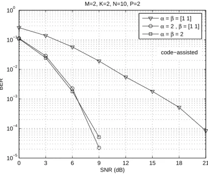
A. Performance of different schemes (M = 2 andM = 4)
First, we consider the code-assisted detection and investigate the performance of some multiple-antenna CDMA schemes for M = 2 and M = 4 transmit antennas. Figure 3 depicts the performance of the 3 different schemes forM = 2. Performance improves when going from full spatial multiplexing (α=β= [1 1]) to full spatial spreading with code reuse (α=β= 2). Note that such a performance gain comes
0 3 6 9 12 15 18 21 10−5
10−4 10−3 10−2 10−1 100
SNR (dB)
BER
M=2, K=2, N=10, P=2
α = β = [1 1]
α = 2 , β = [1 1]
α = β = 2
code−assisted
Fig. 3. Average performance of 3 different transmit schemes withM= 2.
0 5 10 15 20
10−3 10−2 10−1 100
SNR (dB)
BER
M=4, K=2, N=10
α = β = [1 1 1 1], P=4
α = β = [2 1 1], P=3
α = β = [3 1], P=2
α = β = 4, P=2
code−assisted
0 3 6 9 12 15 18 10−4
10−3 10−2 10−1 100
SNR (dB)
BER
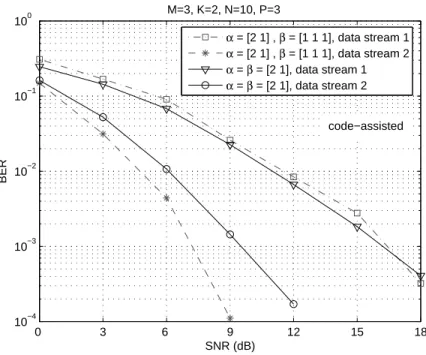
M=3, K=2, N=10, P=3
α = [2 1] , β = [1 1 1], data stream 1
α = [2 1] , β = [1 1 1], data stream 2
α = β = [2 1], data stream 1
α = β = [2 1], data stream 2
code−assisted
Fig. 5. Individual data stream performance for 2 different transmit schemes withM = 3and different choices ofβ.
B. Influence of the code reuse pattern (choice of β)
In Figure 5, we compare the performance of two different schemes combining spatial spreading and spatial multiplexing for M = 3. Both schemes have the same spatial spreading pattern, the difference being on the code reuse/multiplexing pattern. In contrast to previous figures, we plot the individual performance for each data stream in order to verify the influence of code reuse/multiplexing. It can be concluded that the two transmit schemes mainly differ in the performance of the second data stream, which is significantly better as code multiplexing is used. This result confirms that using different codes for transmitting the same data stream across different antennas allows the receiver to use both spatial and code information to distinguish the transmitted substreams, corroborating with [2] and [32].
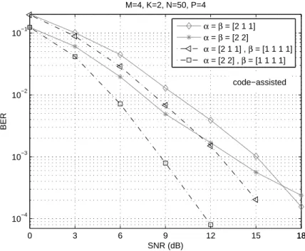
C. Performance over spatially-correlated channel
0 3 6 9 12 15 1818 10−4
10−3 10−2 10−1
SNR (dB)
BER
M=4, K=2, N=50, P=4
α = β = [2 1 1]
α = β = [2 2]
α = [2 1 1] , β = [1 1 1 1]
α = [2 2] , β = [1 1 1 1]
code−assisted
Fig. 6. Average performance of 4 different transmit schemes withM= 4 over a channel with transmit spatial correlation.
receive antennas are uncorrelated. We adopt the following channel model with transmit correlation [33]:
H=HoR1/2
t ,
whereHois a matrix of complex i.i.d. Gaussian variables of unity variance andRtthe transmit covariance
matrix. In this experiment, we assumeM = 4 andRt is given by [34]:
Rt=
1 0.57e−2.25j 0.17e0.02j 0.29e−2.94j 0.57e2.25j 1 0.57e−2.25j 0.17e0.02j 0.17e−0.02j 0.57e2.25j 1 0.57e−2.25j
0.29e2.94j 0.17e−0.02j 0.57e2.25j 1
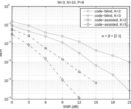
D. Code-blind versus code-assisted detection
In all the previously obtained results, we have considered code-assisted detection by assuming perfectly orthogonal spreading codes (no inter-chip interference). The next results consider the more challenging code-blind detection, where the (effective) spreading codes are unknown to the receiver due to multipath propagation. The effective spreading codes are generated by convolving an orthogonal Hadamard code of lengthP = 32chips with a two-tap multipath channel, the delay between the two taps being equal to two chip periods. At each run, these multipath components are drawn from an i.i.d. complex-valued Gaussian generator. Figure 7 compares the performance of code-blind and code-assisted detection. In this case we use α =β = [2 1]. We can observe a performance loss of the code-blind receiver with respect to the code-assisted one. The performance gap is attributed, in part, to the presence of inter-chip interference and the lack of knowledge of the code matrix which induces more parameters to be estimated by means of the ALS algorithm.
E. Comparison with the optimum ZF receiver
As a reference for comparison, we now consider the performance of the Zero Forcing (ZF) receiver with perfect knowledge of the channel and code matrices. The ZF receiver is compared with the channel-and code-blind ALS receiver. Using our notation, the ZF receiver consists in a single-step estimation of the symbol matrix given by
b
STZF =£¡(CΦ)⋄H¢ΨT¤†X˜2,
H and C being perfectly known. We consider two allocation schemes with α = β = [2 1] (M = 3)
and [2 2] (M = 4). It can be seen from Figure 8 that the gap between ALS and ZF is around 6dB in terms of SNR, for a BER equal to 2·10−2. We can observe that the same performance improvement is
obtained for both ZF and ALS when M is increased.
VIII. CONCLUSION AND PERSPECTIVES
0 3 6 9 12 15 18 21 10−5
10−4 10−3 10−2 10−1 100
SNR (dB)
BER
M=3, N=10, P=8
code−blind, K=2 code−blind, K=3 code−assisted, K=2 code−assisted, K=3
α = β = [2 1]
Fig. 7. Code-assisted versus code-blind detection withM = 3.
0 3 6 9 12 15 18 21 24
10−4 10−3 10−2 10−1 100
SNR (dB)
BER
K=2, N=10, P=4
α = β = [2 1], ALS
α = β = [2 2], ALS
α = β = [2 1], ZF
α = β = [2 2], ZF
M=3
M=4
code−blind
algorithm. Simulation results have shown that remarkable performance is obtained with only two receive antennas and short data blocks. We emphasize that the introduction of the two allocation matrices into the multiple-antenna CDMA model can be further exploited. When some form of channel state information is available at the transmitter, the design of performance-optimized allocation matrices is an interesting issue to be investigated. For a fixed numberM of transmit antennas, we could resort to limited feedback precoding [29], [30] to properly select the two allocation matrices from the finite-set of feasible choices (c.f. Table I forM = 4).
APPENDIX
We demonstrate that the design criterion (20), which results in a partitioned structure for the canonical allocation matrices according to (21)-(22), leads to the uniqueness of S up to column permutation and
scaling while the uniqueness of C exists up to multiplication by a non-singular block-diagonal matrix
and a block-diagonal permutation matrix.
Let us defineC= [. C1, . . . ,CR]∈CP×J andCr= [. Cr,1, . . . ,Cr,J
r]∈C
P×αr withC
r,jr ∈C
P×βr,jr,
jr = 1, . . . , Jr, as the partitioned spreading code matrix. Let us also define H = [H1, . . . ,HR] ∈
CK×M as the partitioned channel matrix. Based on these definitions, we can rewrite (13) in terms of this partitioning as:
X··k = S
à R
X
r=1
ΨrDk(Hr)ΦT
r
!
| {z }
Hk
CT
= SHkCT. (27)
Due to the canonical structure ofΨrandΦr defined in (21)-(22), it follows thatHk is a row-wise
block-diagonal matrix (it has only a single non-zero element per column), the blocks of which are row-vectors:
Hk =
h(1k,1) · · · h(1,J1)
k 0
. ..
0 h(R,1)
k · · · h
(R,JR) k , where
h(r,jr)
k =
βXr,jr
i=1
hk,β
r,jr−1+i ,
withβr,j =
j
P
i=1
βr,i. LetT∈CR×R,U∈CJ×J be non-singular transformation matrices. InsertingTT−1
andUU−1 in (27) yields:
First, note that T−1 acts over the rows ofHk, while U−T acts over the columns of Hk, respectively. It
can be easily checked that T−1 only preserves the row-wise diagonal structure of Hk if it is a diagonal
matrix or a row-permutation of it, which leads to the form (23) ofT. On the other hand, any non-singular
matrix U−T having a block-diagonal structure with blocks U1 ∈CJ1×J1, . . . ,U
R∈CJR×JR, preserves
the structure of Hk which implies a transformational ambiguity over the sets of J1, . . . , JR columns
of C1, . . . ,CR. Note also that the blocksU1, . . .UR can be arbitrarily permuted without changing the
pattern of zeros of Hk, which leads to the form (23) of U.
The block-diagonal transformational ambiguity matrix U=blockdiag(U1, . . . ,UR) exists whenJ >
R (more spreading codes than data streams). In the particular case J =R (one-to-one correspondence
between spreading codes and data streams) with αr = βr, r = 1, . . . , R, Hk is reduced to a diagonal
matrix and the joint uniqueness of S and Cis achieved.
REFERENCES
[1] G. J. Foschini and M. J. Gans, “On limits of wireless communications when using multiple antennas,” Wireless Pers.
Comm., vol. 6, no. 3, pp. 311–335, 1998.
[2] H. Huang, H. Viswanathan, and G. J. Foschini, “Multiple antennas in cellular CDMA systems: transmission, detection, and spectral efficiency,” IEEE Trans. Wireless Commun., vol. 1, no. 3, pp. 383–392, 2002.
[3] S. Sfar, R. D. Murch, and K. B. Letaief, “Layered spacetime multiuser detection over wireless uplink systems,” IEEE
Trans. Wireless Commun., vol. 2, no. 4, pp. 653–668, July 2003.
[4] L. Mailaender, “Linear MIMO equalization for CDMA downlink signals with code reuse,” IEEE Trans. Wireless Commun., vol. 4, no. 5, pp. 2423–2434, Sep. 2005.
[5] T. S. Dharma, A. S. Madhukumar, and A. B. Premkumar, “Layered space-time architecture for MIMO block spread CDMA systems,” IEEE Commun. Letters, vol. 10, no. 2, pp. 70–72, Feb. 2006.
[6] G. D. Golden, G. J. Foschini, R. A. Valenzuela, and P. W. Wolniansky, “Detection algorithm and initial laboratory results using the V-BLAST space-time communications architecture,” Electronics Letters, vol. 35, no. 7, pp. 14–15, Jan. 1999. [7] B. Hochwald, T. L. Marzetta, and C. B. Papadias, “A transmitter diversity scheme for wideband CDMA systems based on
space-time spreading,” IEEE J. Selec. Areas Commun., vol. 19, no. 1, pp. 48–60, Jan. 2001.
[8] R. Doostnejad, T. J. Lim, and E. Sousa, “Space-time spreading codes for a multiuser MIMO system,” in Proc. of 36th
Asilomar Conf. Signals, Syst. Comp., Pacific Grove, USA, Nov. 2002, pp. 1374–1378.
[9] ——, “Space-time multiplexing for MIMO multiuser downlink channels,” IEEE Trans. Wireless Commun., vol. 5, no. 7, pp. 1726–1734, July 2006.
[10] L.-. L. Yang, “MIMO-assisted space-code-division multiple-access: Linear detectors and performance over multipath fading channels,” IEEE J. Selec. Areas Commun., vol. 24, no. 1, pp. 121–131, Jan. 2006.
[11] N. D. Sidiropoulos, G. B. Giannakis, and R. Bro, “Blind PARAFAC receivers for DS-CDMA systems,” IEEE Trans. Sig.
Proc., vol. 48, no. 3, pp. 810–822, Mar. 2000.
[12] N. D. Sidiropoulos and G. Z. Dimic, “Blind multiuser detection in WCDMA systems with large delay spread,” IEEE Sig.
[13] A. de Baynast and L. De Lathauwer, “D´etection autodidacte pour des syst`emes `a acc`es multiple bas´ee sur l’analyse PARAFAC,” in Proc. of XIX GRETSI Symp. Sig. Image Proc., Paris, France, Sep. 2003.
[14] A. L. F. de Almeida, G. Favier, and J. C. M. Mota, “PARAFAC models for wireless communication systems,” in Proc.
Int. Conf. on Physics in Signal and Image processing (PSIP), Toulouse, France, Jan. 31 - Feb. 2 2005.
[15] ——, “PARAFAC-based unified tensor modeling for wireless communication systems with application to blind multiuser equalization,” Signal Processing, vol. 87, no. 2, pp. 337–351, Feb. 2007.
[16] D. Nion and L. De Lathauwer, “A block factor analysis based receiver for blind multi-user access in wireless communications,” in Proc. ICASSP, Toulouse, France, May 2006.
[17] N. D. Sidiropoulos and R. Budampati, “Khatri-Rao space-time codes,” IEEE Trans. Sig. Proc., vol. 50, no. 10, pp. 2377– 2388, 2002.
[18] A. de Baynast, L. De Lathauwer, and B. Aazhang, “Blind PARAFAC receivers for multiple access-multiple antenna systems,” in Proc. VTC Fall, Orlando, USA, Oct. 2003.
[19] A. L. F. de Almeida, G. Favier, and J. C. M. Mota, “Space-time multiplexing codes: A tensor modeling approach,” in
IEEE Int. Workshop on Sig. Proc. Advances in Wireless Commun. (SPAWC), Cannes, France, July 2006.
[20] ——, “Tensor-based space-time multiplexing codes for MIMO-OFDM systems with blind detection,” in IEEE Int. Symp.
Pers. Ind. Mob. Radio Commun. (PIMRC), Helsinki, Finland, September 11-14 2006.
[21] R. Bro, “Multi-way analysis in the food industry: Models, algorithms and applications,” Ph.D. dissertation, University of Amsterdam, Amsterdam, 1998.
[22] H. A. Kiers and A. K. Smilde, “Constrained three-mode factor analysis as a tool for parameter estimation with second-order instrumental data,” Journal of Chemometrics, vol. 12, no. 2, pp. 125–147, Dec. 1998.
[23] J. M. F. ten Berge, “Non-triviality and identification of a constrained Tucker3 analysis,” Journal of Chemometrics, vol. 16, pp. 609–612, 2002.
[24] L. R. Tucker, “Some mathematical notes on three-mode factor analysis,” Psychometrika, vol. 31, pp. 279–311, 1966. [25] R. Bro, R. A. Harshman, and N. D. Sidiropoulos, “Modeling multi-way data with linearly dependent loadings,” KVL
Technical report 176, 2005.
[26] Z. Xu, P. Liu, and X. Wang, “Blind multiuser detection: From MOE to subspace methods,” IEEE Trans. Sig. Proc., vol. 52, no. 2, pp. 91–103, Feb. 2004.
[27] R. A. Harshman, “Foundations of the PARAFAC procedure: Model and conditions for an “explanatory” multi-mode factor analysis,” UCLA Working Papers in Phonetics, vol. 16, pp. 1–84, Dec. 1970.
[28] G. E. Andrews, The theory of partitions. Cambridge, England: Cambridge University Press, 1984.
[29] R. W. Heath and D. J. Love, “Multimode antenna selection for spatial multiplexing systems with linear receivers,” IEEE
Trans. Sig. Proc., vol. 53, no. 8, pp. 3042–3056, Aug. 2005.
[30] D. J. Love and R. W. Heath, “Multimode precoding for MIMO wireless systems,” IEEE Trans. Sig. Proc., vol. 53, no. 10, pp. 3674–3687, Oct. 2005.
[31] N. D. Sidiropoulos and X. Liu, “Cramer-Rao bounds for low-rank decomposition of multidimensional arrays,” IEEE Trans.
Sig. Proc., vol. 49, no. 9, pp. 2074–2086, 2001.
[32] S. Mudulodu and A. J. Paulraj, “A simple multiplexing scheme for MIMO systems using multiple spreading codes,” in
Proc. 34th ASILOMAR Conf. on Signals, Systems and Computers, vol. 1, Pacific Grove, USA, 29 Oct- Nov 1 2000.
[34] D. A. Gore, R. W. Heath Jr., and A. J. Paulraj, “Transmit selection in spatial multiplexing systems,” IEEE Commun. Letters, vol. 6, no. 11, pp. 491–493, 2002.
Andr´e L. F. de Almeida (M’07) was born in Teresina, Brazil, in 1978. He received the B.Sc. and
M.Sc. degrees in electrical engineering from the Federal University of Cear´a, Brazil, in 2001 and 2003, respectively, and the double Ph.D. degree in science and teleinformatics engineering from the University of Nice, Sophia Antipolis, France, and the Federal University of Cear´a, Fortaleza, Brazil, in 2007. He is currently a postdoctoral fellow with the I3S Laboratory, in Sophia Antipolis. He is also affiliated to the Department of Teleinformatics Engineering of the Federal University of Cear´a as an associated researcher with the Wireless Telecom Research Group. His research interest lies in the area of signal processing for communications, and include array processing, blind signal separation and equalization, multiple-antenna techniques, multicarrier and multiuser communications. He has focused on the development of tensor decompositions with applications in MIMO wireless communication systems.
G´erard Favier was born in Avignon, France, in 1949. He received the engineering diplomae from
Jo˜ao Cesar M. Mota was born in Rio de Janeiro, Brazil, in 1954. He received B.Sc. degree in Physics from