January 5
th, 2016
MSc in Finance
- Universidade Católica Portuguesa -
Dissertation
________________________________________________________________
Appropriating the Value of Intellectual Capital:
The Case of U.S. Patents
________________________________________________________________
Tiago Lopes Sequeira
Student Number: 152413028
Joni Kokkonen
Advisor
Dissertation submitted in partial fulfilment of requirements for the degree Master of Science in Finance, at the Universidade Católica Portuguesa (with logo), January 5th, 2016
2
Abstract
This dissertation extends the research on patent value by estimating the value of U.S. patent rights using a new model based on the patent renewal model developed by Schankerman and Pakes (1986) and on the findings of Allison et al. (2004) regarding the endogenous characteristics of valuable patents. The research question of this work aims to find what was the compounded annual growth rate of patent value in the United States in the period between 1981 and 1997? Using patent and renewal data, firstly I estimate the distribution of values of the patents granted in the aforementioned period with the patent renewal model. Secondly I construct an equation using a linear regression, which I named Specific Patent Model, where the independent variables are the patent characteristics and its output is the value of a patent. Thirdly, using the Specific Patent Model I generate the present value of U.S. patent rights granted in the period 1981-1997. Finally, it is presented the historical performance of a portfolio of valuable patents which yields a compounded annual growth rate of 0.7% in the period 1981-1997.
Resumo
A presente dissertação contribui para a literatura existente sobre a valorização de patentes ao estimar o valor das patentes nos Estados Unidos através de um novo modelo baseado no modelo de renovação de patentes desenvolvido por Schankerman e Pakes (1986) e nas descobertas de Allison et al. (2004) relativamente às características endógenas de patentes valiosas. A questão em investigação neste trabalho procura estimar qual a taxa de crescimento anual composta do valor das patentes nos Estados Unidos no período entre 1981 e 1997. Usando informação relativa a patentes e respetivas renovações, eu estimo primeiro através do modelo de renovação de patentes a distribuição do valor de patentes concedidas no período mencionado. De seguida, desenvolvo uma equação através da aplicação de uma regressão linear, à qual chamo de Specific Patent Model, onde as variáveis independentes são as características endógenas das patentes e o resultado da mesma é o valor de uma patente. Em terceiro lugar, aplico o Specific Patent Model para estimar o valor presente das patentes dos Estados Unidos concedidas no período 1981-1997. Por fim, apresento os retornos históricos de um portfolio de patentes valiosas, o qual apresenta uma taxa de crescimento anual composta de 0.7% no período 1981-1997.
3
Contents Page
1. Introduction ... 5
2. IP Rights and Patents: Legal Background ... 7
3. Previous Literature... 10
4. Data ... 13
5. Patent Renewal Model ... 16
6. Present Value of Patent Rights ... 23
7. Patent Value and Characteristics ... 28
8. Time Series of Patents’ Historical Returns ... 37
9. Conclusion ... 41
4
Acknowledgements
The writing and completion of this dissertation would not have been possible without the support and guidance of some people to whom I would like to express my gratitude.
Firstly, I would like to express my sincere gratitude to my advisor Professor Joni Kokkonen for the continuous support, availability and, in particular, for his patience throughout the development of this dissertation. His guidance was critical and I could not have imagined having a better advisor and mentor for my Master of Science dissertation.
My sincere thanks also go to Professor Mark Schankerman of London School of Economics, Mr. Chris Barry, partner at PwC in Boston, U.S. and Dr. Darius Sankey, Managing Director at Ocean Tomo, for their attention and time to reply and answer to my questions and doubts.
I am also particularly grateful to Mr. Erich Spangenberg, not only due to the demonstrated availability and attention, but also due to the sharing of his invaluable expertise in this area. But above all, I am mostly thankful for his words of encouragement and support. They definitely made the difference.
I would also like to thank my current employer Banco de Investimento Global, in particular to the Corporate Finance area to which I report, for the flexibility and support demonstrated, which without it I would not be possible to conclude in due time this work.
I thank my fellow colleagues, and friends, that proved to be critical throughout the development of this dissertation. In particular, I would like to thank Francisco and Frederico for the stimulating discussions, companionship and friendship. I also express my gratitude to Ana, for doubting, to Joana, for motivating me, and to Karina, for her sincere friendship and constant presence even if physically distant.
Last but not the least, I would like to thank my parents for supporting me, with sacrifice, in every way possible throughout the writing of this work and in my life in general.
5
1.
Introduction
In today’s knowledge-based economy, intangible assets such as intellectual property (IP) play a critical role in business activity and economic growth. This is particularly obvious in the case of IP, as these appear to contribute significantly to the market value of firms. Studies show, for example, that tangible assets accounted for only about 25% of the market value of US firms in 2002, suggesting that intangible assets (of which IP is a part) accounted for the remaining 75%. This figure is considerably higher than the 40% of market value that was accounted for by intangibles in 1982 (Kaplan and Norton, 2004).
Furthermore, like other valuable assets, and focusing solely in a single type of IP as representative of the whole class, patents can be also recognised as investment assets because they give owners options on future revenue streams. Consequently, patents should play an important role on its owners’ funding and investment processes (Otsuyama, 2003). Considering the role it has played in terms of innovation and value creation for companies in the last three decades, one would expect to see the value of a hypothetical portfolio of patents to yield higher returns vis-à-vis other more traditional investment asset classes in the past recent years. Therefore, the research question of this dissertation is what was the compounded annual growth rate of patent value in the United States in the period between 1981 and 1997?
While a number of methods have been developed to value patents, one of the most popular and widely used valuation methods is the patent renewal model developed by Schankerman and Pakes (1986), which assumes that patentees derive revenues from their patents only so long as those patents remain in force, i.e. patent holders renew patents only when they are economically valuable. However, this model only reveals the mean and standard deviation of the value of patents granted in a certain year, giving us no information concerning the changes in value of individual patents throughout the years.
So, in order to run a time-series analysis on the value of patents, I study the evolution of a selection of patent characteristics. Following the findings of Allison et al. (2004), patent characteristics such as backward citation, examination period or claims appear to be positively correlated with patent litigation intensity, which is a proxy for patent value.
Using data from 1981 to 1997, I apply the model developed by Schankerman and Pakes (1986) to estimate the distribution of values of the patents granted in that period. Next, I construct an equation using a linear regression, where the independent variables are the patent characteristics and its output is the value of a patent. Since I have patent characteristics data for the entire period,
6
I can estimate the evolution of the changes in values of patents and, consequently, their historical returns.
My empirical findings can be summarised in 5 main results. First, the distribution of the value of patents is positively skewed. Second, the number of claims and the number of examination days is positively correlated to the value of patents. Third, the number of backward citations is negatively correlated to the value of patents. Forth, there are patents with common endogenous characteristics that are more valuable than other patents with different characteristics. Last but not least, in the period 1981-1997, a portfolio constituted by the most valuable patents had a compounded annual growth rate of 0.7%, which answers to the research question.
The rest of the dissertation is organised as follows. Section 2 provides legal background on IP rights and patents. Section 3 is an overview of the previous literature on this topic and section 4 describes the data used to develop this work. Section 5 explains the patent renewal model employed in this dissertation and Section 6 presents the econometric results of the model. Section 7 describes the equation constructed using a linear regression and Section 8 presents the time-series analysis on the value of patents for the period 1981-1997. Section 9 concludes the dissertation.
7
2.
IP Rights and Patents: Legal Background
2.1. Overview
Patent systems have been designed to foster innovation, providing temporary exclusion rights, which raise the private incentives to invest in research and development (R&D), thereby bringing private investment in R&D closer to the socially optimal level and contributing to the diffusion of ideas.
The value of the legal right derives precisely from the existence of this exclusion right and most of its value depends on the patent system that supports those rights. Last, but not least, enforcement, and the costs of enforcement, also have a bearing on the benefits of patent protection.
2.2. U.S. Patent System
In short, the patent application process in the U.S. can be summarised in three different moments. First, the inventor files an application to the U.S. Patent and Trademark Office (USPTO). The application is then examined by the USPTO (in 2010, examination period would last on average 34 months1) to verify if the invention is new, useful and non-obvious, and, if approved, the patent
is granted and the applicant pays the issue and publication fees. Finally, once the patent is granted, the owner of the patent must pay a periodic maintenance fee to keep the patent in force, otherwise the patent protection lapses and the rights provided by a patent are no longer enforceable. Maintenance fees are due three times during the life of a patent, and may be paid without surcharge at 3 to 3.5 years, 7 to 7.5 years, and 11 to 11.5 years after the date of issue. Maintenance fees may also be paid with a surcharge during the "grace periods" at 3.5 to 4 years, 7.5 to 8 years, and 11.5 to 12 years after the date of issue.
Over the past three decades the U.S. patent system went through a series of major changes, both legislative and via legal precedent. One of the most significant legislative changes was brought in by the Bayh-Dole Act in 1980, with the introduction of maintenance fees for all utility patents2
filed on or after December 12, 1980.
Another important legislative change was the establishment in 1982 of the Court of Appeals for the Federal Circuit (CAFC), an important change that fostered the filing of new patents in the
1USPTO, July 8 2010; [accessed 13-09-2015]
http://www.uspto.gov/about/advisory/ppac/Three-TracksExamination(630ext).ppt.
2 Utility patents are issued for the invention of a new and useful process, machine, manufacture, or composition of matter, or a new
8
coming years through the setting of new jurisprudence that expanded decisively the patentable subject matter, from software-related inventions to business methods.
Later, at the Uruguay round of GATT3 in 1994 the U.S. agreed to change the term of patents from
17 years from grant date to 20 years from filing date. This took effect for applications filed on or after June 8, 1995.
Finally, in 2011, the Leahy-Smith America Invents Act (AIA) introduced the most recent significant legislative change. In particular, with the introduction of AIA, the USPTO became free to set the maintenance fees according to other methodologies, while before AIA, these fees were only updated at the Consumer Price Index (CPI) rate. The new fees became active in 2013.
2.3. Patent Litigation
One of the most effective ways of capturing the value of patents is through patent litigation, or more typically, through the threat of patent litigation. Litigation allows the patentees to receive the revenues from owning a patent, which flow from three main sources: exclusion of competitors, licensing of the patent to a firm or firms outside of the patentee’s industry (very common among universities and independent patent owners) and, last but not least, strategic uses of patents, such as avoidance of litigation, cross-licensing or opportunistic patent suits4 based on weak or invalid
patents5.
Even taking into consideration that 99% of patent owners never even bother to file suit to enforce their rights (Lemley, 2001), the fact is that litigated patents are seen by some as signal of value, i.e. a rational agent will only sue someone for infringement if secure of the value and strength of its patent rights.
Particularly interesting is the fact that research shows that litigated patents differ significantly from non-litigated patents. For example, litigated patents have more claims, more backward citations or longer examination periods (Allison et al., 2004).
3 General Agreement on Tariffs and Trade.
4These actions are mainly realised by Non-Practicing Entities (NPEs), which are entities that attempt to enforce patent rights
against third-parties accused of infringing their patent rights.
5 While it is presumed that a patent is valid once it is granted, it may not be always the case. Due to the high amount of yearly patent
filings and the low resources of the patent offices, a defendant (i.e. an entity accused of infringing the patent rights of a third-party) may eventually be able to demonstrate, for example, a printed publication, that was not discovered during the examination period, and that completely describes the invention before the filing date of a certain patent.
9
The endogenous nature of patents therefore seems to have important implications, since if patent applicants are able to recognise which patents are most likely to be litigated, they will invest more effort in, for instance, drafting a patent by including more claims (to broaden the scope of the claims and to make them more resistant to invalidation challenges) and more backward citations (to immunise the patent against possible prior art). This hypothesis is backed by the fact that the number of claims, number of citations, and examination period length have all grown rapidly (Allison and Lemley, 2002), proving the point that applicant can affect effectively the odds of litigation and, as consequence, the value of patents.
10
3.
Previous Literature
What is the value of a patent? This question has attracted a generation of legal scholars, economists and policymakers because the modern patent system presents a seemingly insoluble puzzle. On the one hand, the amount of patenting activity has increased in recent years (Hall, 2004). On the other hand, all empirical evidence demonstrates that the average expected value of a patent is extremely small (Parchomovsky and Wagner, 2005). These persistent and coincident facts fundamentally challenge the traditional understanding of the patent system as generator of incentives to innovate: if patents on inventions have little or no expected economic value, why do individuals and companies patent so heavily? Where does the value of patents lie? This puzzle is referred as the patent paradox.
First, it is important to establish a clear line and clarify the difference between the value of a patent, and the legal rights that come with it, and the value of the underlying invention. In this dissertation, I aim to estimate the value of incremental revenues that patents earn. Patents can provide their owners a degree of market power that carries a stream of profits that exceeds the profits they could earn without patents. This notion of patent value corresponds to the notion of private value of patents.
A distinct notion is the value of the underlying technology. This difference occurs for two reasons. First, innovators also appropriate value from technology by other means such as trade secrecy. The value of patent revenue is incremental, i.e. it is measured relative to an alternative value appropriated by non-patent means. Second, the source of value of patents is endogenous. Patentees can realise efforts in the prosecution of patents and in their enforcement. This effort affects the strength of the patent right and hence the value of the revenues generated.
This endogeneity means that variation in the value of technologies does not necessarily correspond closely to the variation in patent revenues. Therefore, patent value, in the sense used in this dissertation, does not serve well as a measure of “inventive output”. More than analysing patents from an inventors’ perspective, I am interested in finding out the value of patents through the eyes of a financial investor, i.e. patents as an investment asset per se.
But, how to estimate the private value of patents? A number of methods have been developed to value patents but their use is neither widespread nor regular.
Pakes and Schankerman (1984) initiated the research in which maintenance fees are used to calculate the private value and the rate of decay of the revenues generated by patents. The intuition
11
behind this approach is that the patent owners renew their patents as long as the revenues derived from the patents exceed the costs of keeping those patents in force (maintenance fees)6.
The later studies in this line of research used aggregate data, i.e. annual information about the proportion of patents renewed, to infer the value of patents. Schankerman and Pakes (1986) use a model of perfect foresight and determine that the distribution of the value of patents is highly skewed. Their work is a seminal paper and a large part of the subsequent research on private value of patents has employed their model.
Schankerman and Pakes’ (1986) patent renewal model has, nevertheless, limitations because it assumes that revenues are deterministic, i.e. that the patent owner knows with certainty at the time of application for how long he will keep the patent. Pakes (1986) uses a stochastic model of the patent renewal model to estimate the value of patents. This model, in contrast to the model of perfect foresight, allows the patent owner to learn how to use the patent more effectively.
Another limitation of Schankerman and Pakes’ (1986) model is that all patents are generated from the same distribution. Bessen (2006) and Deng (2007) relax this assumption by estimating the model of Schankerman and Pakes (1986) with patent level data. Bessen (2006) uses a cross sectional U.S. patent data and finds that small patentees7 have patents of lower value than large patentees.
Deng (2007) concludes that patent value increases with the economic size of the country.
Bessen (2006) extends the research on patent value of U.S. patents by combining two strands of the literature. One strand uses data on patent renewal decisions, which is the literature already referred previously. The other strand of the literature looks at the relationship between patent value and a variety of patent characteristics. These studies look at correlations between patent and patent owners’ characteristics and variables that should be correlated with patent value such as whether a patent is litigated or not (Allison et al. 2004, Lanjouw and Schankerman 2004, Marco 2005), survey measures of subjective value (Harhoff et al. 1999, 2003), the number of countries in which the patent is filed (Putnam 1996, Lanjouw and Schankerman 2004) and firm market value (Hall et al. 2005). Based on such correlations, it is possible to infer, for example, whether the number of citations made to a given patent is associated in anyway with the value of that same patent (Trajtenberg 1990, Allison et al. 2004, Lanjouw and Schankerman 2004, Marco 2005).
6 As an alternative to this structural approach, researchers have also estimated the relationship between patents and market value of
the firm (Griliches 1981, Cockburn and Griliches 1988, Megna and Klock 1993). Results suggest that patents are valued positively by the market, but there are differences between industries.
7 Small patentees are defined as small businesses, independent inventors and nonprofit organisations. Under the U.S. Code of
Federal Regulations, small business status is granted to firms where the number of employees, including affiliates, does not exceed 500 people.
12
Using these two approaches, the model developed by Bessen (2006) presents several advantages, in particular, it makes it possible to obtain dollar estimates of the incremental effect of, both patent forward and backward citations, and other characteristics on patent value.
More recently, a higher focus on the financial properties of the market for patents has been also developed by a different strand of literature that has approached patents as a financial asset. Under this perspective, cash flows originated by patents, usually obtained through licensing, can be used as underlying flows for patent backed financial instruments, i.e. securitisations.
These financial instruments may, for example, allow companies to raise funds by leveraging on their patents’ portfolio value, which is independent of the valuation of the whole firm (Watanabe, 2004). Another important benefit of the use patents as a financial instrument is the liquidity it provides: upfront payments can be more useful to a company’s funding needs than future royalty streams or delayed sales revenues (Edwards, 2001).
However, assessing the value and risk profile of the patent portfolio is one of the most critical aspects for the development of these financial solutions because of uncertainty in cash flow forecasts and specific risk factors of IP assets like patents. Also, strategic use of patents seems to greatly impact patent value, i.e. each transaction, licensing agreement or other kind of deal involving patents is fundamentally dependent on the stakeholders involved, and their respective strategies, more than on the intrinsic value of the respective patents (Lu, 2013)8. This only further stresses
out the importance of developing a proper valuation method for the setting up of a functioning and liquid patent market.
8 This subjective and relative element that revolves around the valuation of patents was also confirmed by Dr. Darius Sankey,
managing director at Ocean Tomo (an American financial firm specialised in intellectual capital), and by Mr. Erich Spangenberg, founder and previous CEO at IPNav (an American patent-assertion company) in phone interviews and exchange of emails realised throughout November 2014 and April 2015.
13
4.
Data
To develop this work, I used two sets of different but complementary data. One the one hand, I used the database on U.S. patents described in Hall et al. (2001). The data is freely available at the National Bureau of Economic Research (NBER)9. The main data set extends from January 1, 1963
through December 30, 1999 (37 years)10, and comprises detail information of all the utility patents
granted during that period, totalling 2,923,922 patents. In addition to utility patents, there are three other minor patent categories: Design, Reissue, and Plant patents. Since, the overwhelming majority are utility patents (approximately 90% of the patents issued by the USPTO in recent years)11, the data developed in Hall et al. (2001) does not include these other categories.
On the other hand, I used the U.S. Patent Grant Maintenance Fee Events File12 published by the
USPTO, which contains recorded maintenance fee events for patents subject to the payment of maintenance fees filed on or after December 12, 1980 to present. To get the renewal fee costs, I calculated the maintenance fee payment set for the year 201213 (i.e. the last year before the
introduction of the AIA) in 1981 U.S. dollars and indexed it to the registered historical U.S. inflation rate in order to get the maintenance fees for the period between 1981 and 1997. It should be also highlighted that maintenance fees are different depending on the owner of the patent, having the USPTO defined that small patentees paid only 50% of the maintenance fee values defined for large patentees14.
Since patents can be identified through their unique patent identification number it was possible to proceed with the merge of the two datasets to create a single one, where it is possible to observe not only information regarding the endogenous characteristics of a patent (eg. number of claims or backward citations) but as well as the renewal decisions made by the owner of each patent. This is very important since it can shed some light over which endogenous characteristics of a patent make it more prone to be renewed later one. With such database, one is now capable to apply the deterministic renewal model based on the historical observed renewal proportion rates to determine the distribution of values of patents in certain year.
9National Bureau of Economic Research (NBER), May 2012; [accessed 07-02-2015] http://www.nber.org/patents/ 10 NBER has also freely-available a more recent version of this database with data up to date through December 2004. 11 U.S. Patent and Trademark Office (USPTO), October 2013; [accessed 27-09-2015]
http://www.uspto.gov/web/offices/ac/ido/oeip/taf/patdesc.htm
12 U.S. Patent and Trademark Office (USPTO), February 2014; [accessed 07-02-2015]
http://www.uspto.gov/learning-and-resources/electronic-data-products/additional-patent-data-products
13 Setting and Adjusting Patent Fees, Patent and Trademark Office, January 18, 2013, Federal Register / Vol. 78, No. 13, pp. 4225 14 U.S. Patent and Trademark Office (USPTO), November 2013; [accessed 21-10-2015]
14
This imposes other limitation to our data: in order to calculate the average patent value, the model needs to observe the whole future period during which a patent survives to infer the distribution of values. In other words, if one is observing the patents that were granted in 1983, it will be necessary to have observations of the renewal decisions for the next 17 years or, at least, 12 years (if one assumes that after paying for the last maintenance fee, i.e. after 12 years of the granting date, the patent survives until the end of the term). Also, in 1995 the Uruguay round of GATT, as already explained, the statutory term of patents was changed from 17 years from grant date to 20 years from filing date. Since this could potentially affect the final conclusions of this work, I decided to constraint the data to 1997, the year in which the last patents filed before the change in the statutory term took effect were granted.
The dataset that I therefore constructed includes two main sets of variables, those that came from the USPTO (original variables), and those that were created either in Hall et al. (2001) or by myself (constructed variables), amounting to a total of 7.
a) Original Variables: i. Patent number
ii. Application date (starting in December 12, 1980 until June 8, 1995) iii. Grant date (starting in September 1, 1981 until December 30, 1997) iv. Number of claims
v. Maintenance fee events b) Constructed Variables:
i. Number of backward citations (as defined in Hall et al. 2001)
15
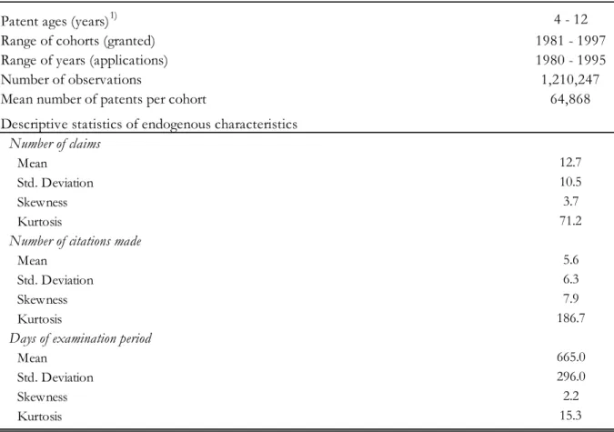
The following table summarises the characteristics of the data employed in this empirical work: Table 2 - U.S. patent data characteristics
Patent ages (years)1) 4 - 12
Range of cohorts (granted) 1981 - 1997
Range of years (applications) 1980 - 1995
Number of observations 1,210,247
Mean number of patents per cohort 64,868
Descriptive statistics of endogenous characteristics Number of claims
Mean 12.7
Std. Deviation 10.5
Skewness 3.7
Kurtosis 71.2
Number of citations made
Mean 5.6
Std. Deviation 6.3
Skewness 7.9
Kurtosis 186.7
Days of examination period
Mean 665.0
Std. Deviation 296.0
Skewness 2.2
Kurtosis 15.3
1) All patents granted survive at least 4 years as the first renewal payment occurs after 4 years of granting date. I have also assumed 12 years as the patent term since there will not be other renewal payment until the patent statutory term year.
16
5.
Patent Renewal Model
This empirical work is based on the patent renewal model developed by Schankerman and Pakes (1986). Patentees derive revenues from their patents only so long as those patents remain in force. If the expected stream of revenues is lower than the renewal fees required to keep the patent alive, patent owners will let the patent expire. The renewal fee varies with the age and with the year in which the patent was granted (from now on defined as cohort). This means that patent renewal and expiration decisions implicitly reflect the value of the patent. The estimation problem of the model is to use data on the proportion of patents renewed and the costs of renewal to estimate the sequence of revenues. The results will allow one to derive the distribution of the value of patent rights and characterise changes that have occurred in it over time.
Consider an agent who holds a patent. Let {𝐶𝑡𝑗} denote the sequence of renewal fees at different
ages, where the subscripts t and j denote the age and cohort of the patent, respectively. The annual economic revenues generated by the patent at age t is denoted by 𝑅𝑡𝑗. These revenues include, for
example, any economic benefits to the patentee that would not have accrued in the absence of the patent right, including licensing agreements, litigation settlements or any other benefit arising from the market power derived from the patent right existence. The sequence {𝑅𝑡𝑗} is assumed to be
known with certainty by the patentee at the time the patent is granted (when patent protection begins). The decision problem is to maximise the discounted value, 𝑉(𝑇), of net revenues from holding the patent by choosing an optimal age to stop paying the renewal fee. Formally, the agent chooses the lifespan of the patent, T, to
𝑚𝑎𝑥
𝑇∈[1,2,…,𝑇̅]𝑉(𝑇) = ∑𝑇𝑡=1(𝑅𝑡𝑗− 𝐶𝑡𝑗)(1 + 𝑖)−𝑡 (1)
Where i is the discount rate and 𝑇̅ is the statutory limit to patent protection. Provided the sequence {𝑅𝑡𝑗− 𝐶𝑡𝑗}𝑡=1𝑇̅ is non-increasing in age15, the optimal lifespan 𝑇∗ is the first age at which 𝑅𝑡𝑗−
𝐶𝑡𝑗 < 0, or if no such 𝑇 ∈ [1,2, … , 𝑇̅] exists, then 𝑇∗ = 𝑇̅. Equivalently, in a world of certainty
with non-increasing net returns, the condition for renewal of the patent at age t is that the annual revenues at least cover the cost of renewal, or
𝑅𝑡𝑗≥ 𝐶𝑡𝑗. (2)
15 The condition that the sequence {𝑅𝑡𝑗− 𝐶𝑡𝑗} is non-increasing in age is sufficient but not necessary. It needs only to hold in the
17
Since renewal fees are increasing in age, a sufficient condition for this renewal rule to be optimal is that the revenues of the patent decay over time.
If the sequence of revenues were the same for all patents in a given cohort, the patents would be cancelled at the same age. Since this is not consistent with the observed renewal curves, the model allows patents in a given cohort to differ in their initial revenues (representing them as random draws from some distribution), but it still assumes that the sequence of decay rates {𝛿𝑡𝑗} is the
same for all patents. The sequence of revenues may depreciate at a constant rate, {𝛿𝑡𝑗} either due
to technological obsolescence (the underlying invention becomes less valuable) or because competitors are able to “invent around” the patent.
The condition for renewal of a patent at age t becomes
𝑅𝑡𝑗≥ 𝐶𝑡𝑗∏𝑡𝜏=1𝑑𝜏𝑗−1, (3)
where 𝑑𝜏𝑗 = 1 − 𝛿𝑡𝑗.
Nevertheless, Schankerman and Pakes (1986) also suggested that the sequence of revenues may also experience some growth as the market and economy expands and/or vary over time in response to changes in economic environment. As result, the net decay rate will reflect both of these factors and, to allow for this, I follow the exact same specification used in the aforementioned paper:
𝑑𝜏𝑗 ≡ (1 − 𝛿𝑡𝑗) = (1 − 𝛿)𝑒𝑥𝑝{𝛽0𝑔𝑡+𝑗+ 𝛽1𝐷1+ 𝛽2𝐷2}, (4) where 𝑔𝑡+𝑗 is the rate of growth of the Gross Domestic Product (GDP) in year t+j, where one
expects 𝛽0 > 0, 𝐷1 = 1 if 1982≤ t+j ≤ 1989 and zero elsewhere, and 𝐷2 = 1 if t+j ≥ 1990 and
zero elsewhere. The time dummy variables 𝐷1 and 𝐷2 are included to capture broad differences in
decay rates across decades which are not reflected in annual movements in aggregate demand. Note that positive values for 𝛽1 or 𝛽2 indicate a decline in the rate of decay during the period between
1982 and 1989 and 1990 and 1997, relative to the year of 1981.
The above specification developed by Schankerman and Pakes (1986) seems, however, to leave aside an important factor that may greatly impact the value of patents and decay rate of its returns according to industry professionals16. If on the one hand, it is true that GDP growth may have a
positive impact in the sequence of revenues of patents by increasing the market size and potential
18
alternatives to the commercial “monetisation” of the patent, on the other hand the exact same GDP growth may also foster innovation. The consequence of this fact is that, if the pace of innovation increases, one would expect to see existent technologies to be replaced by new and better technologies. In other words, innovation cycles and technology replacement in an economy are expected to accelerate the decay rate of the return of current patents.
Therefore, the net decay rate should reflect both of these factors, i.e. the expected positive impact of GDP growth and the expected negative impact of innovation cycles on the sequence of returns derived from patents. Hence, I use the following alternative specification
𝑑′𝜏𝑗 ≡ (1 − 𝛿𝑡𝑗) = (1 − 𝛿)𝑒𝑥𝑝{𝛽0𝑔𝑡+𝑗+ 𝛽1𝑎𝑡+𝑗}, (5)
where 𝑔𝑡+𝑗 is the rate of growth of the GDP in year t+j and 𝑎𝑡+𝑗 represents the rate of growth of
the number of patent filings (used here as a proxy for innovation cycles, i.e. technology creation17)
in year t+j. Moreover, one would expect 𝛽0> 0 (positive effect of GDP growth) and 𝛽1 < 1
(negative effect of innovation cycles).
Regarding the differences in initial revenues among patents in a given cohort, let 𝑓(𝑅0𝑗; 𝜃𝑗) and
𝐹(𝑅0𝑗; 𝜃𝑗) be the density and associated distribution functions of initial revenues, where 𝜃𝑗
denotes a vector of parameters that may vary across cohorts. Then the proportion of patents in cohort j that renew at age t, 𝑃𝑡𝑗, is
𝑃𝑡𝑗 = ∫ 𝑓(𝑅𝑍∞𝑡𝑗 0𝑗; 𝜃𝑗)𝑑𝑅0𝑗 = 1 −𝐹(𝑍𝑡𝑗; 𝜃𝑗), (6)
where 𝑍𝑡𝑗= 𝐶𝑡𝑗∏𝑡𝜏=1𝑑𝜏𝑗−1. Given a functional form for 𝑅0, equation (6) provides the relationship
between the sequence of renewal proportions predicted by the model and the unknown parameters (the vector 𝜃𝑗 and {𝛿𝑡𝑗}).
To complete the specification of the model, it is necessary to select the functional form for 𝑓(𝑅0𝑗; 𝜃𝑗), where 𝜃𝑗 is the vector of parameters for cohort j. Following the findings of
Schankerman and Pakes (1986), I decided to apply a lognormal distribution to the initial distribution of returns, i.e. for 𝑓(𝑅0𝑗; 𝜃𝑗), since the authors found that this was the functional form
that fit the data most closely18.
17 Comanor and Scherer (1969) noted that that patent statistics can be seen as a measure of input to technology creation.
18 Schankerman and Pakes (1986) estimated the model using Pareto, Weibull and lognormal distributions for initial revenues and
the fits obtained by these approaches were compared with each other. The authors find that the lognormal fits better than the Weibull and Pareto, and this result is also corroborated by Schankerman (1998).
19
Assuming, then, that 𝑅0𝑗 distributes lognormally and letting lower case letters denote the
logarithms of upper case ones, one has 𝑟0𝑗~𝑁(𝜇𝑗; 𝜎𝑗) where N(*,*) designates the normal
distribution. In logarithmic form, the decision rule in equation (3) becomes 𝑟0𝑗 ≥ 𝑐𝑡𝑗−
∑𝑡𝜏=1𝑙𝑛(𝑑𝜏𝑗) or, equivalently,
𝑟0𝑗−𝜇𝑗
𝜎𝑗 ≥
𝑐𝑡𝑗−𝜇𝑗−∑𝑡𝜏=1𝑙𝑛(𝑑𝜏𝑗)
𝜎𝑗 (7)
Noting that (𝑟0𝑗 − 𝜇𝑗)/𝜎𝑗 has a standardised normal distribution, the equation for the proportion
of patents in cohort j which have dropped out by age t is given by 𝑦𝑡𝑗 ≡ 𝛷−1(1 − 𝑃 𝑡𝑗) = − 𝜇𝑗 𝜎𝑗+ 1 𝜎𝑗𝑐𝑡𝑗− ∑𝑡𝜏=1𝑙𝑛(𝑑𝜏𝑗) 𝜎𝑗 , (8)
where 𝛷(∙) is the standardised normal distribution function and 𝑦𝑡𝑗 is the standardised normal
distribution function of patents in cohort j which have dropped out by age t.
In writing down the model in (8) I have ignored any sampling errors in the observations on 𝑃𝑡𝑗.
For cohorts as large as those in the sample, as it will be demonstrated in the following section, this variance is essentially zero. In order to allow for discrepancies between the actual and predicted values from the model, I replicated Schankerman and Pakes (1986) that follow Amemiya (1981) by specifying an error term in the renewal rule (7), 𝜀𝑡𝑗.
Finally, given only the proportion of patents renewing in each cohort at each age, it is not possible to estimate a separate lognormal distribution for each cohort. Having assumed the lognormal specification, the mean value of initial revenues in a cohort, 𝑅0𝑗, is given by 𝑒𝜇+1 2⁄ 𝜎
2
and the coefficient of variation is 𝜎. Following Schankerman and Pakes (1986), cohort-specific values of 𝜇 will be allowed but I will maintain a common value of 𝜎 across cohorts.
Incorporating all previous specifications, including specification 𝑑𝜏𝑗, estimated in equation (4), the
model, let’s call it SP model, that is actually estimated and that explains the proportion of patents in cohort j which have dropped out by age t is
𝑦𝑡𝑗 = − 𝜇𝑗 𝜎 + 1 𝜎𝑐𝑡𝑗− 𝑙𝑛(1−𝛿) 𝜎 𝑡 − 𝛽0 𝜎 ∑ 𝑔𝜏+𝑗 𝑡 𝜏=1 −𝛽𝜎1∑𝑡𝜏=1𝐷1 −𝛽𝜎2∑𝑡𝜏=1𝐷2 + 𝜀𝑡𝑗 (9)
where (conditional on t and j) 𝜀𝑡𝑗 is assumed to have mean zero and variance 𝜎𝜀2.
Alternatively to the SP model, if I employ the specification 𝑑′𝜏𝑗, estimated in equation (5), , the
20
𝑦𝑡𝑗 = −𝜇𝜎𝑗+𝜎1𝑐𝑡𝑗−𝑙𝑛(1−𝛿)𝜎 𝑡 −𝛽𝜎0∑𝑡𝜏=1𝑔𝜏+𝑗−𝛽𝜎1∑𝑡𝜏=1𝑎𝜏+𝑗+ 𝜀𝑡𝑗 (10)
Because the error term is heteroskedastic in both models, equations (9) and (10) are estimated by generalised nonlinear least squares.
The estimation problem is now to use data on the proportion of patents renewed and the costs of renewal to estimate the sequence of decay rates, 𝛿, and the parameters characterising the density function of initial revenues, 𝜇𝑗 and 𝜎. These parameters will allow one to derive the distribution
of the value of patent rights.
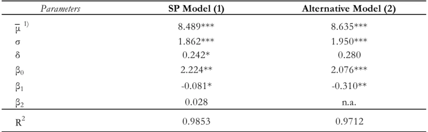
The following table presents the empirical results of both models.
Focusing first in the parameters estimated for the SP Model, the first aspect to be highlighted is the fact that all basic parameters of the model (μ, σ and δ) all have the right sign and all of them are statistically significant. Also, the estimates of σ indicate that the distribution of initial revenues present a high degree of skewness. For the lognormal, this is given by 𝑒𝜎2⁄2 and for SP Model is
5.66, indicating a sharp skewness to the right. This result is in line with previous literature. Table 2 - Parameters estimates of the patent renewal models
Parameters SP Model (1) Alternative Model (2)
μ 1) 8.489*** 8.635*** σ 1.862*** 1.950*** δ 0.242* 0.280 β0 2.224** 2.076*** β1 -0.081* -0.310** β2 0.028 n.a. R2 0.9853 0.9712
Note: a) *** Significance level 1% | b) ** Significance level 5% | c) * Significance level 10% 1) Average of the estimated cohort-specific μj's
The following table describes the parameters estimated of both SP and Alternative models - μ , σ and δ and the coefficients β0, β1 and β2. The μ represents the mean level of the density function of the initial revenues of
patents. The σ is the coefficient of variation of the density function of initial revenues of patents. The δ is the rate at which the sequence of returns generated by patents decay. For the SP Model, the value of δ is allowed to experience some deceleration as GDP of the country expands and/or vary over time in response to changes in economic environment. β0 is the coefficient of the variable g( τ+j) which represents the rate of growth of GDP in year (τ+j) . β1 is the coefficient of the dummy variable D1 which equals to 1 if 1982 ≤ τ+j ≤ 1989. β2 is the coefficient of the dummy variable D2 which equals to 1 if τ+j ≥ 1990 and zero elsewhere. For the Alternative Model, the value of δ is allowed to experience some deceleration as GDP of the country expands and/or acceleration in response to innovation cycles. β0 is the coefficient of the variable g(τ+j) which represents the rate of growth of GDP in year (τ+j) . β1 is the coefficient of a(τ+j) which represents the rate of growth of the number of patent filings in year (τ+j) .
21
One of the premises of the model is that the rate of decay depends inversely on the rate of growth of the GDP. This hypothesis is indeed confirmed by the parameters estimated, with 𝛽0, the
coefficient of the variable g(τ+j) which represents the rate of growth of GDP in year (τ+j), having a
positive sign, i.e. 𝛽0 > 0. Moreover, the null hypothesis 𝛽0 = 0 can be rejected. Consequently, one
can conclude that the implied quantitative impact of GDP growth on the decay rate is quite big, at least at the economy-wide level of aggregation.
Concerning the decade effects over the decay rate in SP Model, 𝛽1 and 𝛽2 present mixed signs,
with former having a negative sign which accelerates the decay rate of patent returns. This may result from a period of higher innovation (increasing obsolesce of existent technology) or economic downturn (decreasing market size). The latter presents a positive sign, which may be explained by the exact opposite effects. However, while 𝛽1 is statically significant, for 𝛽2 it is not possible to
reject the null hypothesis that 𝛽2 = 0. This may be interpreted as that the period after 1990 had
simply no effect over the decay rate of patent returns.
Finally, the estimates of the decay rate do indicate a rapid decline in the private returns from holding patents, at least when compared to the rate of decay generally assumed for the physical productivity of traditional capital goods: rate of decay of traditional capital are assumed to be in the range 4-10%19 which compares to the rate of decay estimated for SP Model of 24.2%. This result is not
surprising since the decay in the returns earned from holding patents is not due to any decline in the physical productivity of the knowledge embodied in them, but rather to two other related points: it is difficult to establish and maintain effective proprietary rights over the knowledge, and new inventions are developed which displace the original ones20.
Focusing now in the parameters estimated for the Alternative Model, the first aspect to be highlighted is the fact that all basic parameters of the model (μ, σ and δ) have the right sign and all, with the exception of the parameter δ, are statistically significant. The fact that the parameter δ, as opposed to the SP Model, is not significant means that under the Alternative Model the decay rate has no effect on the sequence of returns. This result is nevertheless highly unlikely in reality, since one would expect to observe any asset to be depreciated at a certain rate. This could be justified by the incapacity of the lognormal distribution to explain the sequence of returns with the evolution of innovation cycles.
19 The commonly assumed rate of decay of the knowledge produced by firms is between 4% and 7% (Mansfield 1968). Griliches
(1980), noting some of the conceptual distinctions between the rates of decay in traditional capital and in research, assumes an upper bound of 10% for the latter.
22
The estimates of σ indicate that the distribution of initial revenues present a high degree of skewness just like in the SP Model. For the Alternative Model is 6.69, indicating a sharp skewness to the right. This result is in line with both previous literature and SP Model.
Also in accordance with the estimates in SP Model, the hypothesis advanced that the rate of decay depends inversely on the rate of growth of the market (𝛽0 > 0) is supported by the data: 𝛽0 has
the expected sign and the null hypothesis 𝛽0 = 0 can be rejected. In fact, the value of 𝛽0 is even
higher than the one of SP Model, which means that under the Alternative Model, the impact of the GDP growth rate in the evolution of returns is more noticeable.
The main assumption of the Alternative Model was that innovation cycles accelerate the rate of decay of patent returns. The 𝛽1 in Alternative Model is the coefficient of a(τ+j) which represents the
rate of growth of the number of patent filing in year (τ+j). If innovation cycle do accelerate the rate of decay then the coefficient 𝛽1 should exhibit a negative sign. The hypothesis advanced seems
indeed to receive support of the data, with 𝛽1= -0.310 in Alternative Model; as the rate of filings
increases, so does the pace of technology creation and replacement, leading to an increasing pressure over the returns of the existing patents.
23
6.
Present Value of Patent Rights
The lognormal distribution on 𝑅0𝑗 induces a distribution the present value of patent rights. Having
concluded the estimation problem described in previous section, the parameter estimates in Table 2 (𝛿, 𝜇 and 𝜎) can be now used to derive the distribution of the value of patent rights.
Recalling equation (1), the present value of patent rights for a single patent, denoted by 𝑉(𝑇), is given by 𝑉(𝑇) = ∑(𝑅𝑡𝑗− 𝐶𝑡𝑗) 𝑇∗ 𝑡=1 (1 + 𝑖)−𝑡= ∑[𝑅 0𝑗(1 − 𝛿)𝑡− 𝐶𝑡𝑗](1 + 𝑖)−𝑡 𝑇∗ 𝑡=1
where 𝑅𝑡𝑗− 𝐶𝑡𝑗 is the net revenue from holding the patent belonging to cohort j during age t, i is
the discount rate21, 𝛿 is the appropriate decay rate, and 𝑇∗ is the optimal lifespan of the patent as
defined in section 5.
Next, I generate 100,000 pseudo-random variables from a lognormal distribution on 𝑅0
parameterised by the estimated μ, mean level of the density function of the initial revenues of patents, and σ, coefficient of variation of the density function of initial revenues of patents. For each draw the estimates of δ and the renewal fees22 are added to the equation to compute the
optimal expiration date according to the renewal rule and generate the associated net value of patent rights for that draw. In this way the entire distribution of the value of patent rights is constructed. I repeated the above process for the parameters estimated by both SP and Alternative Models. The following table presents the descriptive statistics of the value of the patent rights in the U.S. for a single cohort, which for the sake of simplicity I assumed to be the cohort of year 1982.
21 Following Schankerman and Pakes (1986), I assumed the discount rate to be equal to 10%.
22 Since this is a random sample, I cannot define which returns are produced by patents owned by small or large entities. For the
sake of simplicity, I assumed a weighted average fee for large and small entity as if it was a single and unique type of maintenance fee.
24
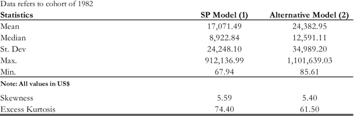
The first striking difference between the present value of the patent rights estimated with the parameters obtained from the SP Model compared to the present value estimated with the parameters obtained from the Alternative Model is that the latter has a higher mean value vis-à-vis the former. This result should not be surprising since, as it is possible to verify in Table 2, the decay rate, δ, was not statistically significant, meaning that it cannot be rejected the hypothesis that it is equal to 0. If that is the case, i.e. if the returns of the patent do not decay, it logically follows that the present value of the future returns generated by the Alternative Model will be higher than the ones generated by the SP Model.
Also, it is possible to observe in Table 3 a large gap between the median and the mean value, confirmed by both models, a direct consequence of the registered sharp skewness and high kurtosis. More importantly, the most interesting feature of these distributions is their positive skewness, meaning that the right tail of the distribution is longer and the mass of the distribution is concentrated to the left of the mean value. In other words, there is a dense concentration of patent rights with very little economic value, in line with the findings of Schankerman and Pakes (1986) for the United Kindgom, Germany and France.
While, on the one hand, the median value is slightly higher compared with the values estimated in previous studies, like Bessen (2006)23, the mean value, on the other hand, exhibits a much lower
23 Median value of $4,792, in 1982 U.S. dollars.
Table 3 - U.S. patent descriptive statistics
Data refers to cohort of 1982
Statistics SP Model (1) Alternative Model (2)
Mean 17,071.49 24,382.95
Median 8,922.84 12,591.11
St. Dev 24,248.10 34,989.20
Max. 912,136.99 1,101,639.03
Min. 67.94 85.61
Note: All values in US$
Skewness 5.59 5.40
Excess Kurtosis 74.40 61.50
The following table presents the descriptive statistics of the present value of patent rights, V(T). The present value of the patent right may differ depending from which model, SP Model or Alternative Model, were the parameters μ , σ and δ obtained from. The distribution of the present value of patent rights is induced by the log-normal distribution of R0j, which is parameterised by the estimated μ and σ. For the SP Model, the mean value
of the patent rights obtained in 1982 is $17,071 and the most valuable patent obtained in 1982 was worth $912,137. For the Alternative Model, the mean value of the patent rights obtained in 1982 is $24,071 and the most valuable patent obtained in 1982 was worth $1,101,639.
25
value when compared with the same study. Bessen (2006) estimates a mean value for patents granted to U.S. patentees of $52,201 in 1982 U.S. dollars, which compares to $17,071 and $24,383 in 1982 U.S. dollars generated by SP Model and Alternative Model respectively. These are interesting results because Bessen estimates the value of patents granted in 1991, while I’m using the cohort of 1982. Which seems to imply that patent rights have become more valuable throughout the decade that separates these two years (this conclusion is not corroborated by the SP Model, with this model estimating the value of 1991 cohort to be $15,519. The fact that Bessen (2006) estimates his model with patent level data instead of generating all patents from the same distribution may explain the differences).
A closer look to the estimates of the decay rate, δ, and of the coefficient of variation, σ, used to calculate 𝑉(𝑇) may help to understand this apparent increase in value between the patent value estimated by Bessen (2006) for the 1991 cohort and the value estimated for the 1982 cohort. While it is true that the estimations of coefficient of variation, σ, in both SP Model and Alternative Model are in line with the findings of Bessen (2006) – 1.86 compared to 1.86 and 1.95 in SP Model and Alternative Model respectively – one cannot say the same about the estimation of the decay rate,
δ. The value calculated by Bessen (2006) for δ is considerably lower (14%) than the ones estimated
in this work – 24% and 28% in SP Model and Alternative Model respectively. This result can be interpreted either in two ways:
1) Between the years of 1982 and 1991 the level of innovation decreased significantly, lowering the pace of technology waves and replacement by newer one;
2) The endogenous characteristics of patent rights and the overall legal framework have become stronger and better defined, increasing the liquidity and value of patent rights. The results mentioned above also seem to be supported by the observed evolution of the proportion of patents renewed in the period 1982-1991, presented in Table 4.
Table 4 - Proportion of patents renewed in a selection of cohorts
Data refer to 1982, 1991 and 1997 cohorts
Cohort 4th year 8th year 12th year
1982 83% 63% 37%
1991 79% 58% 41%
1997 88% 69% 52%
Renewal Proportion (%)
The following table presents the evolution of the proportion of patents in cohorts 1982, 1991 and 1997, the last cohort available, that renew at each renewal payment age.
26
From Table 4 it is possible to confirm that the decay rate of the 1991 cohort is lower compared to the 1982 cohort, resulting in higher proportion of renewals by the last renewal payment age, year 12. However, this is only clearly observable after the 8th year from the granting date, because before
that year it was, in fact, the opposite trend that was true: younger patents, i.e. more recent cohorts, had lower renewal rates. So, what was the trigger driving this change?
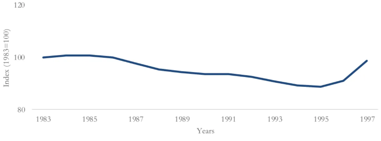
Between 1982 and 1999 (cohort of 1991 plus 8 years) the explanation that seems to fit the story is that innovation did, in fact, speed up during the 1980s, causing the development of new technologies and consequent replacement of older ones. The result was that the younger patents presented lower renewal proportions when compared with its older peers. Figure 1 shows exactly this: the number of yearly patent filings in the U.S. almost doubled between 1981 and 1997.
After 1999 the story seems to change, with the cohort of 1991 having more renewals by the 12th
year than the proportion of renewals observed by the 12th year in cohort of 1982. Also, if one looks
to the 1997 cohort, the 4th year is the year 2001, and, in this case, the renewal proportions are always
higher throughout the entire patent statutory term vis-à-vis the older patents.
A reasonable explanation might be related to the publishing of the Intellectual Property and Communications Omnibus Reform Act of 1999. Under this new legislation, patent applications filed on or after the 29th of November 2000 must be published after 18 months from the
application’s date (i.e. published even before they are actually granted). The impact of such legislation might have implications, not only on the coming patents, but also over the existent ones. For example, if I need to take a decision on whether to renew a patent or not, it would be extremely useful to know what kind of claims the coming patents have in order to maximise the utility of my
Figure 1 - Evolution of U.S. patents filings in the period 1981-1997
80 100 120 140 160 180 1981 1983 1985 1987 1989 1991 1993 1995 1997 In dex ( 19 81 =1 00 ) Years
27
patent. The endogenous characteristics of patent rights and the overall legal framework seem to have become stronger and better defined, increasing the liquidity and value of patent rights. Should be noted nevertheless that these are aggregate results; i.e. the above models only return the average value of patent rights granted in a given year. In particular, one limitation about estimating the value of patents based on renewal data is that patentee renewal decisions do not reveal, at least directly, the value of the most valuable patents. Most valuable patents in the upper tail of the distribution are renewed to full term, meaning that although the estimates of median values are based on an observed distribution, estimates of mean patent value are based on an extrapolation. In other words, it is assumed that the distribution observed among expiring patents (in this case, a lognormal distribution) is the same for all patents, including the most highly valued patents. Consequently, if the true distribution is not log normal, these estimates may be off. Also, this model is not suited to give information regarding any individual and specific patent, nor any information about the evolution of the patent characteristics over time. Which means that to answer to the research question of the dissertation, what was the compounded annual growth rate of patent value in the United States in the period between 1981 and 1997, another strategy needs to constructed.
28
7.
Patent Value and Characteristics
In the previous section I calculated the present value of patent rights. However, the value obtained is based on aggregated results which does not allow me to observe the changes in value of individual patents throughout the years.
As seen in section 3, many researchers have related value to patent characteristic and from this fact results that a patentee, aware that some patents are more valuable than others, may take efforts to make sure that the patent is more successfully applied. These efforts include making more backward citations and claims in the patent application, for example.
In an attempt to estimate the changes in value of individual patents throughout the years, I developed a new model to estimate the value of single and specific patents dependent on their characteristics.
In order to develop this new model, let’s call it Specific Patent Model, I followed the findings of Allison et al. (2004) and, taking into consideration data constraints, I ended up selecting three characteristics: backward citations, number of claims and examination period.
The idea that supports this new model is quite simple: if certain endogenous characteristics are correlated to value and if only valuable patents are renewed, then one should expect to observe a higher concentration of valuable endogenous characteristics amongst the most renewed patents. To test this hypothesis, I generated Q-Q (quantile-to-quantile) plots24, presented below in Figure
2, in order to compare the distributions of each characteristic against the distribution of the patent values estimated with the patent renewal model25. If the distributions of each characteristic match
the distribution of the patent values then the Q-Q plot would closely follow a 45º line.
24 A Q–Q plot is a plot of the quantiles of two distributions against each other.
29 Figure 2 - Q-Q Plots
a) R0 and Citations
b) R0 and Claims
c) R0 and Examination Days
0 30,000 60,000 90,000 120,000 150,000 0 2 4 6 8 R0 Citations 0 30,000 60,000 90,000 120,000 150,000 0 10 20 30 40 R0 Claims 0 30,000 60,000 90,000 120,000 150,000 300 400 500 600 700 R0 Examination Days
30
All the previous three graphs plotted in Figure 2 are flatter than the 45º line, meaning that the distributions of the theoretical quantiles (patent values) are more dispersed than the distribution of the sample quantiles (patent characteristics). In other words, this is a clear signal of positive skewness of the sample quantiles, in line with the findings described in Table 3 in section 6. Having confirmed the skewed nature of the distribution of the endogenous characteristics, I move to the development of the Specific Patent Model.
Let’s recall equation (9) derived from the SP Model:
𝑦𝑡𝑗 = −𝜇𝑗 𝜎 + 1 𝜎𝑐𝑡𝑗− 𝑙𝑛(1 − 𝛿) 𝜎 𝑡 − 𝛽0 𝜎 ∑ 𝑔𝜏+𝑗 𝑡 𝜏=1 −𝛽1 𝜎 ∑ 𝐷1 𝑡 𝜏=1 −𝛽2 𝜎 ∑ 𝐷2 𝑡 𝜏=1 + 𝜀𝑡𝑗
By re-arranging equation (9) and, once again, letting lower case letters denote the logarithms of upper case ones, one can derive
𝜇𝑡𝑗 = (−𝑦𝑡𝑗+𝜎1× 𝑐𝑡𝑗−𝑙𝑛(1−𝛿)𝜎 𝑡 −𝛽0
𝜎 ∑ 𝑔𝜏+𝑗
𝑡
𝜏=1 −𝛽𝜎1∑𝑡𝜏=1𝐷1−𝛽𝜎2∑𝑡𝜏=1𝐷2) × 𝜎, (11)
where 𝜇𝑡𝑗 is the represents the mean level of the density function of the initial revenues of patents
of cohort j at age t.
Having previously found the variables estimated by the SP Model (see Table 2 in section 5), I plug the correspondent variables into equation (11) in order to get the mean value, 𝜇𝑡𝑗, for each t for
every cohort between 1981 and 1997. Once this process is complete, I end up with 51 observations of 𝜇𝑡𝑗.
After having obtained the values of 𝜇𝑡𝑗, I sorted the average values of the three selected
endogenous characteristics, backward citations, claims and examination days, correspondent to each age t for every cohort j. According to the hypothesis that the distributions of the characteristics and patent value match, one should expect to observe characteristics with higher average values concentrated in later renewal decision stages. As t increases, one would expect to see an increase in the average value of the characteristics as well, independent of the selected cohort. Indeed, it is exactly this pattern that is verifiable across all cohort with the exception of patents granted in 1981 and 1982, where values in t = 2 are higher than in t = 3.
Values estimated for the mean level of the density function of the initial revenues of patents of cohort j at age t, 𝜇𝑡𝑗, when sorted, decrease as t increases, and this pattern is common to the
31
of patent rights supported in the idea that higher proportion of patent renewals signals higher value of patent rights. If renewal proportions decrease in t, and since only few patents survive until the term, then, according to the model, 𝜇𝑡𝑗 should also be lower as t increases. Yet, the fact that there
are fewer patents, and as result lower aggregate value, as t moves forward, does not imply that the average value of the surviving patents is also lower.
The fact that 𝜇𝑡𝑗 decreases in t while endogenous characteristics increase in t can be problematic
since it puts in jeopardy the positive correlation between patent characteristics and value. To solve this issue, it is necessary to apply an adjustment factor to the average values of the characteristics to replicate the pattern found in 𝜇𝑡𝑗. To do it, I calculate the average value across all cohorts of the
proportion of patents renewed at each t. Once this process is done, I estimate the difference between the average value of the proportion of renewals and the estimated cohort j-specific renewal proportion at each age t. In the end, the adjustment factor is given by
𝐴𝑑𝑗𝑢𝑠𝑡𝑚𝑒𝑛𝑡 𝐹𝑎𝑐𝑡𝑜𝑟 = 1 − (𝑃̅ − 𝑃𝑡 𝑡𝑗) (12)
where P represents the proportion of renewals of the surviving patents. By multiplying the adjustment factor to the endogenous characteristics in each t and for evert cohort, I forced the value of the characteristics to adjust in t for every cohort, matching the same pattern as the one observed in 𝜇𝑡𝑗.
Having applied the adjustment factor to the average values of the characteristics and having assumed the lognormal specification, I sorted the mean value of initial revenues for each t across every cohort, 𝜔𝑡𝑗.
Once this process is completed, I end up with the average endogenous characteristics of backward citations, claims and examination days and the mean value of initial revenues, 𝜔𝑡𝑗, sorted by age t
and cohort j. To establish now a relation between 𝜔𝑡𝑗 and the selected endogenous characteristics,
I ran a linear regression26.
Before employing the linear regression, and in order to normalise the data, I first define 𝑙𝑛(𝜔𝑡𝑗),
the natural logarithms of 𝜔𝑡𝑗, as the dependent variable and cl, ct and experiod, the natural logarithms
of the endogenous characteristics Claims, Backward Citations, and Examination Period, as the independent variables.
26 I have also replicated this process, namely equation (11), with data generated by the Alternative Model in order to get the
32
Linear regressions, in particular, are effective in quantifying the strength of the relationship between variables with the advantage of being easier to fit than models which are non-linearly related to their parameters.
The mean value of the initial revenues for a single patent under the Specific Patent Model, denoted by 𝑟0′, is given by
𝑟0′ = 𝑏 + 𝛾0𝑐𝑙 + 𝛾1𝑐𝑡 + 𝛾2𝑒𝑥𝑑𝑎𝑦𝑠 + 𝜀 (13),
where 𝜀 is assumed to have mean zero and variance 𝜎𝜀2.
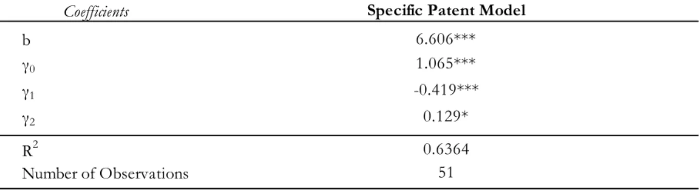
The following table presents the empirical results of the Specific Patent Model.
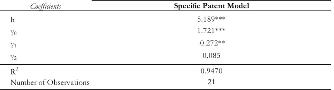
The first aspect to be highlighted in Table 5 is the statistical significance of all parameters that compose equation (13), with the Specific Patent Model presenting a high explanatory power (R2=0.6364).
The coefficients 𝛾0 and 𝛾2 have positive values as expected and in accordance with previous
literature (see section 3), meaning that the higher number of claims and the number of examination days, the higher the mean value of the initial revenues of a patent. In particular, a 10% increase in the number of claims results in an 11% increase in the initial revenues (calculated as 1.1𝛾0 − 1 =
11%), and a 10% increase in the number of examination days results in an almost insignificant 1% increase in the initial revenues (calculated as 1.1𝛾2 − 1 = 1%).
Table 5 - Parameters estimates of the Specific Patent Model Data refers to the period 1981-1997
Coefficients b γ0 γ1 γ2 R2 Number of Observations
Note: a) *** Significance level 1% | b) ** Significance level 5% | c) * Significance level 10%
0.6364 51
Specific Patent Model
6.606*** 1.065*** -0.419***
0.129*
The following table describes the parameters estimated by the Specific Patent Model - b and the coefficients γ0,
γ1 and γ2. The b represents the intercept of the linear regression. γ0 is the coefficient of the variable cl , which
represents the number of claims. The γ1 is the coefficient of the variable ct , which represents the number of backward citations. γ2 is the coefficient of the variable exdays, which represents the examination days.