Adaptive Kalman based forecasting for electric load and distributed generation

(1)

UNIVERSIDADE DE BRAS´ILIA FACULDADE DE TECNOLOGIA

DEPARTAMENTO DE ENGENHARIA EL´ETRICA

ADAPTIVE KALMAN BASED FORECASTING FOR

ELECTRIC LOAD AND DISTRIBUTED GENERATION

LUCAS DANTAS XAVIER RIBEIRO

ORIENTADOR: JO ˜AO PAULO CARVALHO LUSTOSA DA COSTA

DISSERTAÇ ÃO DE MESTRADO EM ENGENHARIA ELÉTRICA

PUBLICAC¸ ˜AO: 659/2017 DM PPGEE

(2)

(3)

UNIVERSIDADE DE BRAS´ILIA FACULDADE DE TECNOLOGIA

DEPARTAMENTO DE ENGENHARIA EL´ETRICA

ADAPTIVE KALMAN BASED FORECASTING FOR

ELECTRIC LOAD AND DISTRIBUTED GENERATION

LUCAS DANTAS XAVIER RIBEIRO

DISSERTAC¸ ˜AO DE MESTRADO SUBMETIDA AO DEPARTAMENTO

DE ENGENHARIA EL´ETRICA DA FACULDADE DE TECNOLOGIA

DA UNIVERSIDADE DE BRASÍLIA, COMO PARTE DOS REQUISITOS NECESS ÁRIOS PARA A OBTENÇ ÃO DO GRAU DE MESTRE EM EN-GENHARIA ELÉTRICA.

APROVADA POR:

Prof. Jo˜ao Paulo Carvalho Lustosa da Costa, Dr.-Ing. (ENE-UnB, Frau-nhofer IIS e TU Ilmenau)

(Orientador)

Prof. Rafael Tim´oteo de Sousa J´unior, Dr. (ENE-UnB) (Examinador Interno)

Wesley Fernando Usida, Dr. (ANEEL) (Examinador Externo)

(4)

FICHA CATALOGR ´AFICA

RIBEIRO, LUCAS DANTAS XAVIER

Adaptive Kalman based Forecasting for electric load

and distributed generation. [Distrito Federal] 2017.

xvii, 290p., 297 mm (ENE/FT/UnB, Mestre, Engenharia El´etrica, 2017) Disserta¸c˜ao de Mestrado - Universidade de Bras´ılia.

Faculdade de Tecnologia. Departamento de Engenharia El´etrica.

1. Kalman Filter 2. Principal Component Analysis 3. Load Forecasting 4. Distributed Energy Resources I. ENC/FT/UnB II. T´ıtulo (s´erie)

REFERˆENCIA BIBLIOGR ´AFICA

RIBEIRO., L. D. X. (2017). Adaptive Kalman based Forecasting for electric load and distributed generation. Disserta¸cão de Mestrado em Engenharia Elétrica, Pu-blica¸cão 659/2017 DM PPGEE, Departamento de Engenharia Elétrica, Universidade de Bras´ılia, Bras´ılia, DF, 290p.

CESS ˜AO DE DIREITOS

NOME DO AUTOR: Lucas Dantas Xavier Ribeiro.

TÍTULO DA DISSERTAÇ ÃO DE MESTRADO:Adaptive Kalman based Forecasting for electric load and distributed generation.

GRAU / ANO: Mestre / 2017 ´

E concedida à Universidade de Bras´ılia permissão para reproduzir cópias desta dis-serta¸cão de mestrado e para emprestar ou vender tais cópias somente para propósitos acadêmicos e cient´ıficos. O autor reserva outros direitos de publica¸cão e nenhuma parte desta disserta¸cão de mestrado pode ser reproduzida sem a autoriza¸cão por escrito do autor.

Lucas Dantas Xavier Ribeiro

SGAN 911 M´odulo F, Bloco H, Apartamento 12, Asa Norte 70790-110 Bras´ılia - DF - Brasil.

(5)

DEDICAT ´

ORIA

Alis volat propriis. Per aspera, ad astra.

(6)

AGRADECIMENTOS

Primeiramente `a Deus `

A minha fam´ılia por todo o cuidado, carinho e pela educa¸cão que me foi dada. Sem vocês jamais teria chegado neste ponto. Agrade¸co à minha mãe por toda a dedica¸cão e por ser meu maior exemplo de vida. Ao meu pai por ter me ensinado muitos dos valores que me definem como homem. À minha irmã pela amizade e carinho por todos estes anos. À minha querida tia Jailma por ser a melhor tia do mundo. À minha avó Nina por ser uma segunda mãe para mim.

Agrade¸co ao meu orientador, Prof. Jo˜ao Paulo, por todo o aux´ılio dis-pensado na orienta¸c˜ao deste trabalho, em particular pela ajuda e est´ımulo `

as publica¸cões. Agrade¸co ao meu amigo Jayme Milanezi Júnior por ser a pessoa que mais me auxiliou nesta atividade de pesquisa. Também agrade¸co a meus amigos Márcio Ven´ıcio Pilar de Alcântara e Elton Mário de Lima por terem me auxiliado com opiniões, artigos e com o empréstimo de livros didáticos. Todos vocês contribu´ıram para a realiza¸cão desta disserta¸cão.

Aos meus amigos da Agência Nacional de Energia Elétrica (ANEEL), em particular á equipe da Superintendência de Pesquisa e Desenvolvimento e Eficiência Energética (SPE). Agrade¸co à agência por ter me concedido li-cen¸ca para cursar disciplinas no horário da manhã. Ao Superintendente, Máximo Luiz Pompermayer agrade¸co a confian¸ca em mim depositada. Igual-mente, agrade¸co a Aurélio Calheiros de Melo Júnior, a Fábio Stacke Silva, a Carmen Silvia Sanches e a Sheyla Maria das Neves Damasceno. Amigos que sempre me ajudaram a conciliar o trabalho com este curso de p´ os-gradua¸cão. Aos demais amigos da SPE e da ANEEL, o meu agradecimento pela amizade e companheirismo, gra¸cas a vocês dou muito valor ao nosso ambiente de trabalho.

Agrade¸co ao Prof. José Luiz Cerda-Arias e ao colega de pós-gradua¸cão Marcos Vin´ıcius Vieira, que foram responsáveis pela obten¸cão dos dados de demanda elétrica de Leipzig e de Bras´ılia, respectivamente. Ao Prof. Edison Pignaton pelas sugestões e pela aten¸cão dispensada em uma fase crucial deste trabalho. Ao colega Ricardo Kehrle Miranda pela ajuda e parceria dispensada.

(7)

(8)

RESUMO

PREVIS ÃO ADAPTATIVA DE CARGA E DE GERAÇ ÃO DISTRIBUÍDA BASEADA EM FILTROS DE KALMAN

Autor: Lucas Dantas Xavier Ribeiro

Orientador: João Paulo Carvalho Lustosa da Costa Programa de Pós-gradua¸cão em Engenharia Elétrica Bras´ılia, abril de 2017

O desenvolvimento econômico está relacionado à disponibilidade de energia elétrica, especialmente em virtude da dependência quase total que a maioria das indústrias e dos servi¸cos essenciais têm de seu uso. A disponibilidade de energia perene, barata e confiável é de primordial importância econômica.

Dado que o conjunto de requerimentos encontrados pelas companhias de distribui¸cão constitui um cenário complexo, ferramentas robustas de previsão de demanda são ne-cessárias para implementar planos de expansão e opera¸cões eficientes e razoáveis. A inser¸cão de gera¸cão distribu´ıda adiciona um novo n´ıvel de complexidade a esta ta-refa, pois não somente a gera¸cão descentralizada diminui a carga de modo aleatório e intermitente, como também inevitavelmente produz altera¸cões nas séries históricas de carga usadas para fazer as previsões. Ambos os efeitos agem no sentido de aumentar os erros de predi¸cão no curto e no longo prazo, amea¸cando a eficiência operacional e, no pior caso, a estabilidade do sistema.

Este trabalho apresenta a previsão de carga e gera¸cão como um problema de estima¸cão dinâmica de estado via filtros adaptativos de Kalman. As variáveis a serem estima-das são das demandas de base, média e de pico, assim como a gera¸cão fotovoltaica. Como medi¸cões e observa¸cões, são utilizadas previsões de tempo, datas e eventos de calendário, tarifas de eletricidade, ´ındices e estimativas econômicas e demográficas. Combina¸cões preprocessadas destas medi¸cões são usadas como as variáveis de entrada para a previsão.

A metodologia proposta foi comparada com outras técnicas do estado da arte, sendo os desempenhos avaliados com base nos critérios de Erro Médio Quadrático (MSE), Raiz do Erro Médio Quadrático (RMSE), Coeficiente de correla¸cão, Erro Médio Per-centual (MAPE), Erro Médio Absoluto (MAE), Erro Médio de Tendência (MBE), Erro Máximo Absoluto (MXE) e Erro Máximo Percentual (MPE). Na maioria dos cenários

(9)

analisados, o sistema de predi¸cão adaptativo proposto superou as técnicas de referência baseadas em redes neurais e espa¸co de estados.

(10)

ABSTRACT

ADAPTIVE KALMAN BASED FORECASTING FOR ELECTRIC LOAD AND DISTRIBUTED GENERATION

Author: Lucas Dantas Xavier Ribeiro

Supervisor: João Paulo Carvalho Lustosa da Costa Programa de Pós-gradua¸cão em Engenharia Elétrica Bras´ılia, abril de 2017

Economic development is related to the availability of electricity, especially because most industries and basic services depend almost entirely on its use. The availability of a source of continuous, cheap, and reliable energy is of foremost economic importance. Since the set of requirements faced by power distribution utilities assemble a complex scenario, robust load forecasting tools are needed to implement efficient and reasonable expansion and operation plans.

The introduction of distributed generation adds a new level of complexity to this task, as not only the decentralized generation reduces load in a random and intermittent way, but also inevitably embeds in the historic loads used to forecast. Both effects act to increase prediction errors in short and long term, jeopardizing operational efficiency and, in worst case, system reliability.

This work presents the load and generation forecasting as a dynamic state estimation problem by means of Kalman adaptive filters. The variables to be estimated are daily base, average and peak electric load, as well as PV generation. As measurements and observations, this work uses weather forecasts, calendar dates and events, energy tariffs, economical and demographic indexes and estimatives. Preprocessed combinations of these measurements are the input variables employed for forecasting.

The proposed methodology is compared with other state-of-art techniques, the perfor-mances evaluated with base in error performance criteria such as Mean Squared Error (MSE), Root Mean Squared Error (RMSE), Correlation coefficient, Mean Average Percentual Error (MAPE), Mean Absolute Error (MAE), Mean Bias Error (MAE), Maximum Absolute Error (MXE) and Maximum Percentual Error (MPE). In most evaluated scenarios, the proposed adaptive prediction system outperforms the bench-mark techniques, based on state space and neural networks.

(11)

LIST OF TABLES

1.1 Suprimento de Eletricidade Dom´estico, PIB e popula¸c˜ao de 2000 a 2015

- Mundo e Alemanha . . . 2

2.1 Worldwide and Domestic German Energy Supply (DES), German Gross Domestic Product (GDP) and Population from 2000 to 2015 . . . 2

3.1 Common link functions of the Exponential family . . . 17

3.2 List of METAR’s measurements and observations . . . 26

3.3 Approximate calculation of the heating degree-days . . . 31

3.4 Approximate calculation of the cooling degree-days . . . 32

3.5 Approximate calculation of the heating degree-days . . . 37

3.6 Photometric and corresponding radiometric units . . . 44

3.7 List of Socioeconomic variables obtained per Case study . . . 48

3.8 List of event variables . . . 52

3.9 Inputs and outputs per PV forecasting step . . . 62

4.1 Listing of the candidate input variables . . . 77

4.2 Inputs and outputs per predicting phase . . . 84

5.1 Error metrics for Base load, Substation S1 . . . 101

5.2 Error metrics for Average load, Substation S1 . . . 102

5.3 Error metrics for Average load, Substation S1 (continuation) . . . 103

5.4 Error metrics for Peak load, Substation S1 . . . 104

5.8 Error metrics for Peak load, Substation S2 (continuation) . . . 109

(15)

5.37 Error metrics for Base load, Brasilia first period . . . 141

5.38 Error metrics for Average load, Brasilia first period . . . 142

5.39 Error metrics for Peak load, Brasilia first period . . . 143

5.40 Error metrics for Base load, Brasilia second period . . . 146

5.41 Error metrics for Average load, Brasilia second period . . . 147

5.42 Error metrics for Peak load, Brasilia second period . . . 148

5.43 Error metrics for Peak load, Brasilia second period (continuation) . . . 149

5.44 PV Systems in site A1 . . . 153

5.45 Results for Systems A1a and A1b, single station . . . 155

5.46 Results for Systems A1c and A1d, single station . . . 155

5.47 Results for Systems A1a and A1b, multiple stations . . . 157

5.48 Results for Systems A1c and A1d, multiple stations . . . 157

(16)

5.53 Results for Systems A3a, A3b and A3c, single station . . . 166

5.55 Results for System A4a, single station . . . 170

5.56 Results for System A4a, multiple stations . . . 171

5.58 Results for System A5a, single station . . . 173

5.59 Results for System A5a, multiple stations . . . 174

5.61 Results for Systems A6a and A6b,single station . . . 177

5.64 Results for Systems A7a and A7b, single station . . . 181

6.1 ANN and Kalman filter processing time ratio. . . 185

6.2 Summary of results - Leipzig scenario. Best methods per substation and load type. . . 186

6.3 Summary of results - Leipzig scenario. Best input sets per substation and load type. . . 186

6.4 Summary of results - Brasilia scenarios. Best methods per substation and load type. . . 187

6.5 Summary of results - Brasilia scenarios. Best input sets per substation and load type. . . 187

6.6 Summary of results - PV forecasting scenarios. Best methods per system.188 B.1 Coefficients for the Equation of Time and for the Sun declination . . . 227

B.2 Typical sample values of Albedo for different surfaces/enviroments . . . 234

B.3 SEDES2 Coefficients by wavelenght (1st part) . . . 237

B.4 SEDES2 Coefficients by wavelenght (2nd part) . . . 238

(17)

LIST OF FIGURES

1.1 Oferta de eletricidade e gera¸cão renovável alemã em TWh, entre 2001 e 2015. Fonte: [110], licen¸ca Creative Commons by SA 4.0. . . 4 1.2 Esquema simplificado de um sistema elétrico com gera¸cão distribu´ıda . 5 1.3 Percentual de energia renovável no consumo l´ıquido de eletricidade na

Alemanha, de 2005 a 2015. Em 2015 as fontes renováveis supriram 38 % do consumo. Fonte: [105] . . . 6 1.4 Evolu¸cão trimestral do número de unidades de gera¸cão distribu´ıda

co-nectadas às redes de distribui¸cão brasileiras. Fonte: ANEEL . . . 7 1.5 Capacidade instalada (esquerda) e número de unidades conectadas

(di-reita) no Brasil, divididas por fonte prim´aria de energia. Fonte: ANEEL 7 1.6 Custo m´edio l´ıquido do sistema FV para o consumidor, considerando

sistemas para instala¸c˜ao em telhados com potˆencia nominal entre 10 kWp e 100 kWp. Fonte: [105] . . . 8 2.1 German and European photovoltaic (PV) generated power in MW, between

2001 and 2015. Source: [110], Creative Commons license by SA 4.0. . . 3 2.2 Simplified schematic of a electric power system with Distributed Energy

Resources . . . 5 2.3 Percentage of renewable energy in Germany’s net electricity

consump-tion, from 2005 to 2015. In 2015 the renewable sources accounted for 38 % of the consumption. Source: [105] . . . 6 2.4 Quarterly evolution of the number of DG units connected to the

Brazi-lian grid. Source: ANEEL. . . 6 2.5 Installed capacity (left) and number of connections (right) of DG units

in Brazil, by energy source. Source: ANEEL. . . 7 2.6 Average net system price to customer, for rooftop systems with nominal

(18)

3.1 From top left to bottom left: Load as an electric device, a building, a distribution feeder, a distribution substation, a citywide distribution grid and as national load centers. In specific contexts, load can refer to any of this six levels of aggregation. . . 13 3.2 Comparison of the forecasting error among five scenarios. The intrisic

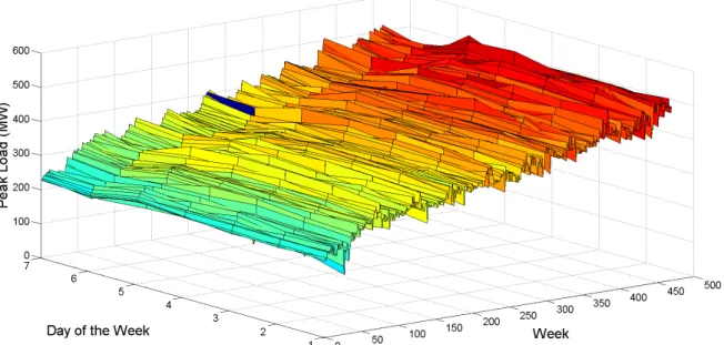
noise, which is oftenly related to measurement errors, is independent of the forecasting algorithm and is constant among all cases. . . 20 3.3 Peak load in Brasilia from 2001 to 2010. Weakly variation is visible in

y axis (Day of the week), while the demand growth trend superposed to the seasonal variation is visible in the x axis (Week). . . 21 3.4 Factors and their main effects over the electricity demand. . . 24 3.5 This chart is a summary of the human comfort zone as a function of

ambient conditions (weather and climate). Modified from the original in

Wikimedia Commons, license CC BY-SA 3.0

(http://creativecommons.org/licenses/by-sa/3.0), acessible at https://commons.wikimedia.org/wiki/File%3APsychrometricChart.SeaLevel.SI.svg. 28 3.6 Scatter plot of mean temperature and mean demand in Megawatts (MW).

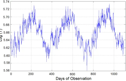
Five polynomial best fitting showcases the large residuals and diverse possibilities from nonlinear behavior. . . 29 3.7 Logarithm of the absolute temperature, as measured in Leipzig from

2001 to 2003 . . . 30 3.8 Heating Degree Days at 18 Celsius reference, as measured in Leipzig

from the 2001 to 2003. The heating peaks are measured in the winter season. . . 31 3.9 Scatter plot of HDD and mean demand in MW, as measured in Leipzig

from the 2001 to 2003. Five polynomial best fitting curves showcase the more straightforward dependence, yet nonlinear. . . 32 3.10 Scatter plot of CDD and peak demand in MW, as measured in Bras´ılia

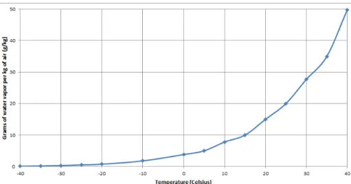
from 2001 to 2003. Because the large number of noncorrelated points stays at zero degree-days, they do not affect the determination of the CDD coefficient. . . 33 3.11 Maximum water vapor content of air as a function of temperature. This

is the reference to calculation of Relative Humidity. . . 35 3.12 Natural illumination model. The five “window” surfaces are used to

ap-proximate the sunlight incident into buildings and open spaces. Modified

from original provided by By TWCarlson [CC BY-SA 3.0

(http://creativecommons.org/licenses/by-sa/3.0)], via Wikimedia Commons. Accessible at https://upload.wikimedia.org/wikipedia/commons/f/f7/Azimuth-Altitude schematic.svg . . . 41

(19)

3.13 (a) Cross section through a human eye. (b) Schematic view of the retina and its photoreceptors (adapted from Encyclopedia Brittannica, 1994 edition) . . . 42 3.14 Normalized spectral sensivity of rod and cone cells. By Maxim Razin

[CC BY-SA 3.0 (http://creativecommons.org/licenses/by-sa/3.0)], via

Wikimedia Commons. Accessible at https://commons.wikimedia.org/wiki/File:Cone-response.svg . . . 43

3.15 Eye sensivity function. The values of CIE 1978 V (λ) are shown in the left-hand ordenate, while the correspondent luminous efficacy (conver-sion factor for Watts to lumens) are shown in the right-hand orde-nate. Both are maximum in 555 nm wavelenght. By Jordanwesthoff (Own work) [CC BY-SA 3.0

(http://creativecommons.org/licenses/by-sa/3.0)], via Wikimedia Commons. Accessible at https://commons.wikimedia.org/wiki/File%3AHuman photopic response.jpg 45

3.16 Natural solar irradiation. The roof and four wall surfaces are used to approximate the heat absorption by irradiation into buildings. Modified

from original provided by By TWCarlson [CC BY-SA 3.0

(http://creativecommons.org/licenses/by-sa/3.0)], via Wikimedia Commons. Accessible at https://upload.wikimedia.org/wikipedia/commons/f/f7/Azimuth-Altitude schematic.svg . . . 46

3.17 60 day moving average of electricity tariffs in Bras´ılia, in Brazilian Reais (BRL) per MWh, by consumer class . . . 51 3.18 Global cumulative growth of PV capacity. Source: reproduced from IEA

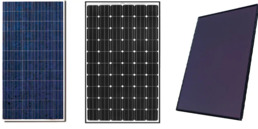
Solar photovoltaic roadmap 2014 [51] . . . 58 3.19 Apparent difference between module types. From left to right.

Poly-crystaline Silicon module, MonoPoly-crystaline Silicon and Thin Film module. 59 3.20 Box diagram of the solar photovoltaic simulational framework . . . 61 3.21 Sun azimuth angle and elevation angle. Azimuth reference is the

geo-graphical north pole. Modified from original provided by By TWCarlson [CC BY-SA 3.0 (http://creativecommons.org/licenses/by-sa/3.0)], via

Wikimedia Commons. Accessible at https://upload.wikimedia.org/wikipedia/commons/f/f7/Azimuth-Altitude schematic.svg . . . 63

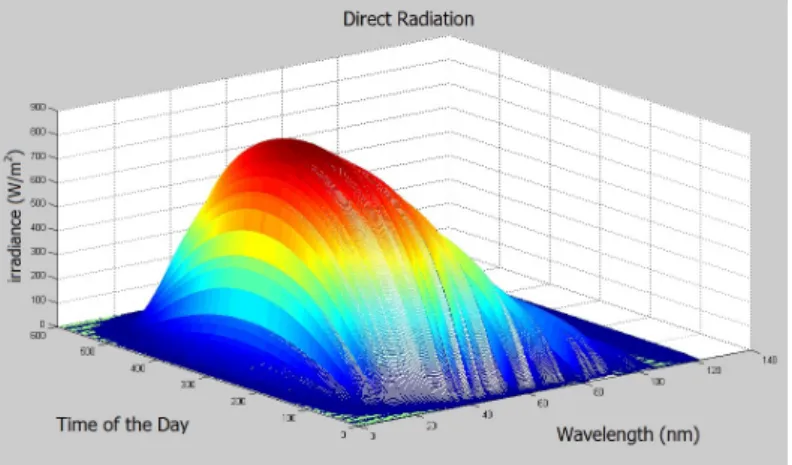
3.22 Direct Normal Irradiation as a function of time and wavelength . . . . 64 3.23 Schematic of a crystalline silicon solar panel . . . 68 3.24 Typical spectral response of the polycrystalline silicon cell (blue) and

(20)

3.25 Example of Extraterrestrial Solar irradiation (AM0), ASTM Standard Spectrum (AM1,5) in cloudless sky and Absorbed Spectrum by a typical poly-Si cell (AM1,5) . . . 70 4.1 Proposed data model for Load forecasting . . . 76 4.2 Correlation between several candidate variables and peak demand, which

corresponds to the projection in the planes x = 0 or y = 0 . . . 79 4.3 Correlation between the 126 selected variables and peak demand, which

corresponds to the projection in the planes x = 0 or y = 0 . . . 80 4.4 Box Diagram of the proposed Kalman based predicting scheme . . . . 84 4.5 Proposed data model for Load forecasting . . . 93 5.1 Leipzig population and population growth rate from 1990 to 2015. The

1999 growth peak is due to the incorporation of surrounding towns. Credits: EUROSTATs . . . 98 5.2 Locations of the eight substations in Leipzig. Credits: Jayme Milanezi

Jr. [73] . . . 98 5.3 Evolution of electric load in Substation S1, from 2001 to 2004. Base

load is plotted in black, Average load in blue and Peak load in red. . . 99 5.4 Sum of the Total Squared Error for the 8 substations as a function of

Model Order. The minimum is achieved when the Order is set to 7. . . 100 5.5 Prediction (red line) plotted against the measured base load in

Substa-tion S1 (blue line) over 360 days of observaSubsta-tion. . . 102 5.6 Prediction (red line) plotted against the measured average load in

Subs-tation S1 (blue line) over 360 days of observation. . . 103 5.7 Prediction (red line) plotted against the measured peak load in

Substa-tion S1 (blue line) over 360 days of observaSubsta-tion. . . 105 5.8 Prediction (red line) plotted against the measured base load in

(21)

5.13 Prediction (red line) plotted against the measured peak load in Substa-tion S3 (blue line) over 360 days of observaSubsta-tion. . . 113 5.14 Prediction (red line) plotted against the measured base load in

(22)

5.31 Prediction (red line) plotted against the measured peak load in Substa-tion S9 (blue line) over 360 days of observaSubsta-tion. . . 137 5.32 Evolution of Brasilia’s population and GDP between 1999 and 2014.

Credits: CODEPLAN . . . 138 5.33 Location of Juscelino Kubistchek International Airport relative to

Bra-silia and the Federal District. Credits: Google Maps . . . 139 5.34 Evolution of electric load in Brasilia, from July 2001 to December 2003.

Base load is plotted in black, Average load in blue and Peak load in red. 139 5.35 Total Squared Error for the second scenario, as a function of Model

Order. The minimum is achieved when the Order is set to 8. . . 140 5.36 Prediction (red line) plotted against the measured base load in Brasilia

(2001-2003 period) over 360 days of observation. . . 141 5.37 Prediction (red line) plotted against the measured average load (blue

line) in Brasilia (2001-2003 period) over 360 days of observation. . . . 143 5.38 Prediction (red line) plotted against the measured peak load (blue line)

in Brasilia (2001-2003 period) over 360 days of observation. . . 144 5.39 Evolution of electric load in Brasilia, from February 2004 to June 2010.

Base load is plotted in black, Average load in blue and Peak load in red. Two outliers in the Peak load are not visible in this graph. . . 145 5.40 Total Squared Error for the second scenario, as a function of Model

Order. The minimum is achieved when the Order is set to 8. . . 145 5.41 Prediction (red line) plotted against the measured base load (blue line)

in Brasilia (2004-2010 period) over 360 days of observation. . . 147 5.42 Prediction (red line) plotted against the measured average load (blue

line) in Brasilia (2004-2010 period) over 360 days of observation. . . . 148 5.43 Prediction (red line) plotted against the measured peak load (blue line)

in Brasilia (2004-2010 period) over 360 days of observation. . . 149 5.44 The European sites selected for the forecast. Credits: Google Earth. . . 150 5.45 Location of the Australian sites selected for the forecast. Credits: Google

Earth . . . 152 5.46 Location of the North American generation site selected for the forecast.

Credits: Google Earth . . . 153 5.47 Site A1 and the six airport weather stations used for the forecast.

Cre-dits: Google Earth . . . 154 5.48 Error graphs for forecasts in Systems A1a and A1b, from left to right.

(23)

5.49 Error graphs for forecasts in Systems A1c and A1d, from left to right. Single station . . . 156 5.50 Error graphs for forecasts in Systems A1a and A1b, from left to right.

Multiple stations. . . 158 5.51 Error graphs for forecasts in Systems A1c and A1d, from left to right.

Multiple stations. . . 158 5.52 Prediction (red line) plotted against the measured PV Generation (blue

line) in site A1a over 360 days of observation. . . 159 5.53 Prediction (red line) plotted against the measured PV Generation (blue

line) in site A1b over 360 days of observation. . . 159 5.54 Prediction (red line) plotted against the measured PV Generation (blue

line) in site A1c over 360 days of observation. . . 160 5.55 Prediction (red line) plotted against the measured PV Generation (blue

line) in site A1d over 360 days of observation. . . 160 5.56 Site A2 and the two airport weather stations used for the forecast.

Single station. . . 162 5.58 Error graphs for forecasts in Systems A2a and A2b, from left to right.

line) in site A2b over 360 days of observation. . . 164 5.61 Site A3 and the airport weather station used for the forecast. Credits:

Google Earth . . . 165 5.62 Error graphs for forecasts in Systems A3a (top left), A3b (top right) and

A3c (bottom). Single station. . . 167 5.63 Prediction (red line) plotted against the measured PV Generation (blue

line) in site A3b over 360 days of observation. . . 168 5.65 Prediction (red line) plotted against the measured PV Generation (blue

line) in site A3c over 360 days of observation. . . 169 5.66 Site A4 and the six airport weather stations used for the forecast.

Cre-dits: Google Earth . . . 170 5.67 Error graphs for forecasts in System A4a. Single station. . . 171

(24)

5.68 Error graphs for forecasts in System A4a. Multiple stations. . . 171 5.69 Prediction (red line) plotted against the measured PV Generation (blue

line) in site A4a over 360 days of observation. . . 172 5.70 Site A5 and the six airport weather stations used for the forecast.

Cre-dits: Google Earth . . . 173 5.71 Error graphs for forecasts in System A5a. Single station. . . 174 5.72 Error graphs for forecasts in System A5a. Multiple stations. . . 174 5.73 Prediction (red line) plotted against the measured PV Generation (blue

line) in site A5a over 360 days of observation. . . 175 5.74 Site A6 and the six airport weather stations used for the forecast.

Single station. . . 177 5.76 Error graphs for forecasts in Systems A6a and A6b, from left to right.

line) in site A6b over 360 days of observation. . . 179 5.79 Site A7 and the two airport weather stations used for the forecast.

Single stations. . . 181 5.81 Error graphs for forecasts in Systems A6a and A6b, from left to right.

line) in site A7b over 360 days of observation. . . 183 6.1 Scatter plot of the ANN to Kalman filter processing time ratio, as a

function of the input size. . . 185 6.2 Principal components horizontally sorted in decreasing order of singular

value. There are noticeable discontinuities around the first, the seventh and eighth component. Model order in this case has been selected as 7. 190 6.3 Principal components horizontally sorted in decreasing order of singular

value. There are noticeable discontinuities around the first and the tenth component. Model order in this case has been selected as 10. . . 190

(25)

B.1 Electromagnetic wave propagating from left to right. The electric field is in a vertical plane and the magnetic field in a horizontal plane. The electric and magnetic fields are always in phase and at 90 degrees to each other. . . 216 B.2 Electromagnetic spectrum expressed in terms of energy and wavelength.

In detail, the visible spectrum perceived by the human eyes as colors. . 216 B.3 Atmospheric Opacity as a function of the EM radiation wavelength.

Note that the atmosphere is highly transparent to the visible spectrum. 217 B.4 Solar irradiance at space (yellow) and at sea level (red). For comparison,

the gray line corresponds to the blackbody spectrum at 5778 K. . . 218 B.5 Dates for seasons, apoapsis and periapsis of Earth’s orbit. The elliptical

form is exagerated. . . 219 B.6 Analemma plotted as seen at noon GMT from the Royal Observatory,

Greenwich (latitude 51.48◦ north, longitude 0.0015◦ west). . . 220 B.7 CERES-Aqua 2003-2004 mean annual clear sky and total sky albedo.

Clear sky albedo is the fraction of the incoming solar radiation that is re-flected back into space by regions of the Earth on cloud-free days. Total

sky albedo include cloudy days. Data source: http://daac.gsfc.nasa.gov/giovanni/ 221

B.8 Solar Azimuth and Elevation (complement of Zenith Angle) angles. Pa-nel Azimuth and tilt angles. Azimuth reference is the geographical south pole. . . 223 B.9 Burning a dry leaf with a magnifier lens. The bright spot over the

smo-king leaf is concentrated Direct irradiation of the Sun. The daylit ground is illuminated by the Global irradiance. The shadowed areas are dimly il-luminated by the Diffuse irradiation component. Photography credits go

to Dave Gough, available at https://www.flickr.com/photos/spacepleb/1505372433 (CC BY 2.0 license) . . . 224 B.10 SPCTRL2 Extraterrestial Solar Radiation. . . 228 D.1 Perceptron with 3 inputs and bias. From left to right: inputs, weights,

summation block, activation function and output. . . 246 D.2 Schematic of Multilayer Perceptron. From left to right, the input layer

(26)

LIST OF SYMBOLS, NOMENCLATURES AND ACRONYMS

ANEEL: Acronym for Agˆencia Nacional de Energia El´etrica, the Brazilian electricity regulatory agency.

AM: Air Mass.

ANN: Artificial Neural Network. AR: Auto-Regressive model.

ARMA: Auto-Regressive Moving Average model.

ARMAX: Auto-Regressive Moving Average with eXogenous inputs model. ARX: Auto-Regressive with eXogenous inputs model.

BP: Back-Propagation, an ANN training method. CDD: Cooling Degree-Days.

CIE: Commission Internationale de l’´Eclairage (International Commission on Illumi-nation).

cov(X, Y ): Covariance of X and Y.

DER: Distributed Energy Resources. Refers to energy supplies, storage and power sources positioned closer to demand centers, frequently installed in customer sites. DG: Distributed Generation. Refers to power sources positioned closer to demand centers, frequently installed in customer sites. Unlike DER, does not refers to storage technologies.

ELD: Enthalpy Latent Days.

GMT: Greenwich Mean Time, the mean solar time at the Royal Observatory in Gre-enwich, London.

HDD: Heating Degree-Days.

Iλ: Irradiance at wavelength λ, the power irradiated over a surface by a light source in the λ wavelength per unity of area.

(27)

KF: Kalman Filter.

λ: Wavelength of electromagnetic irradiation. MAE: Mean Absolute Error metric.

MAPE: Mean Average Percentual Error metric. MBE: Mean Bias Error metric.

METAR: METeorological Aerodrome Report. Acronym to a format for reporting we-ather information used by airports and pilots worldwide.

MLP: MultiLayer Perceptron, an ANN architecture. MPE: Maximum Percentual Error metric.

MSE: Mean Squared Error metric. MXE: MaXimum absolute Error metric. PCA: Principal Component Analysis.

PV: PhotoVoltaic. Physical property that enables direct conversion of light into elec-tricity using semiconducting materials.

φλ: Illuminance at wavelength λ, the luminous flux over a surface by a light source in the λ wavelength per unity of area.

E(f ), f , µf: Expected value of the stochastic function f [k]. RMSE: Acronym for the Root Mean Squared Error metric. σf: Standard deviation of stochastic function f [k].

SVD: Singular Value Decomposition.

V ar(f ): Variance of stochastic function f [k]. z: Notation for a scalar z.

z[k]: Value of the scalar function z at discrete time step k. ˆ

(28)

Z: Notation for a vector Z.

Z[k]: Value of the vectorial function Z at discrete time step k. ˆ

Z[k]: Prediction for the value of vectorial function Z at discrete time step k. Z: Notation for a matrix Z.

Z[k]: Value of the matricial function Z at discrete time step k. ˆ

(29)

1 INTRODUC

¸ ˜

AO

Mundialmente, o desenvolvimento econômico depende diretamente da disponibilidade de energia elétrica, especialmente em virtude da dependência quase total que a maioria das industrias e dos servi¸cos essenciais têm de seu uso. A disponibilidade de uma fonte de energia perene, barata e confiável é de primordial importância econômica.

Grandes montantes do suprimento energético são mundialmente destinados a setores energeticamente intensivos, como o tratamento de água, irriga¸cão, industria de trans-forma¸cão e transportes. Em particular, os pa´ıses mais ricos tem as maiores demandas energéticas por habitante, uma vez que o Produto Interno Bruto (PIB) é altamente correlacionado com a utiliza¸cão de energia.

Esta dependência pode ser linearmente modelada ao se considerar dados de 2003 a 2007 [2]. A rela¸cão causal entre crescimento econômico, caracterizado em diversos indicado-res, e o consumo de eletricidade é investigado em inúmeros artigos. O estudo apresen-tado em [22] conclui que a causalidade é mais forte em paises desenvolvidos da OECD. Várias variáveis são utilizadas para indicar as dependências entre consumo de energia e atividades econômicas: Produto Interno Bruto (PIB), popula¸cão e ´ındices de pre¸cos [7]. Em [11], testes de Granger indicam rela¸cão de causalidade do consumo energético para a renda na Índia e na Indonésia, ao passo que o mesmo teste aponta para uma rela¸cão bidirecional para a Tailândia e as Filipinas. Esta dependência bidirecional aponta para um sistema retroalimentado, no qual a disponibilidade de um suprimento barato de energia promove o crescimento econômico, e então a atividade econômica aquecida de-manda um consumo maior de eletricidade e/ou melhoria da eficiência energética. Deste ponto de vista, as demandas energéticas devem ser analisadas não somente como um servi¸co essencial, mas também como um indicador econômico.

(30)

Tabela 1.1: Suprimento de Eletricidade Dom´estico, PIB e popula¸c˜ao de 2000 a 2015 - Mundo e Alemanha

DES DES PIB Pop. DES / Capita

Ano Mundo Alemanha Alemanha Alemanha Mundo — Alemanha (TWh) (TWh) 109 _US$ ₁₀6_Hab. _{TWh /10}6_Hab.

2000 15406,03 579,6 1949,95 82,21 2,52 — 7,05 2001 15638,45 585,1 1950,65 82,35 2,52 — 7,11 2002 16190,43 587,4 2079,14 82,49 2,58 — 7,12 2003 16793,16 600,7 2505,73 82,53 2,64 — 7,28 2004 17572,76 610,2 2819,25 82,52 2,73 — 7,39 2005 18333,46 614,1 2861,41 82,47 2,81 — 7,45 2006 19030,16 619,8 3002,45 82,38 2,89 — 7,52 2007 19922,93 621,5 3439,95 82,27 2,98 — 7,55 2008 20283,94 618,2 3752,37 82,11 3,00 — 7,53 2009 20123,69 581,4 3418,01 81,90 2,94 — 7,10 2010 21404,5 615,0 3417,30 81,78 3,09 — 7,52 2011 22050,91 606,1 3757,46 81,80 3,15 — 7,41 2012 22504,33 605,7 3543,98 80,43 3,17 — 7,53 2013 23092,66 603,8 3752,51 82,13 3,22 — 7,35 2014 24240,89 591,1 3879,28 80,98 3,34 — 7,30 2015 25893,62 595,1 3363,45 81,41 3,52 — 7,31

Os dados na Tabela 1.1 extra´ıdos de [4, 3] mostram a evolu¸cão de três indicadores relacionados às economias mundial e alemã no per´ıodo de 2000 a 2012. As primeiras duas colunas na Tabela 1.1 correspondem ao Suprimento de Eletricidade Doméstico no mundo e na Alemanha (DES), do inglês Domestic Energy Supply. A terceira e quarta coluna apresentam o PIB e a popula¸cão em milhões de habitantes. A última coluna na Tabela 1.1 apresenta o suprimento de eletricidade per capita (DES/capita) para o mundo e para a Alemanha. É importante observar que a popula¸cão alemã manteve-se praticamente constante, embora o montante de energia suprida tenha crescido.

O consumo por habitante na Tabela 1.1 segue uma curva ascendente no per´ıodo entre 2000-2015, e isto indica a necessidade de cont´ınuos investimentos na rede elétrica. A previsão de carga mostra-se, portanto, como uma ferramenta essencial para as compa-nhias de distribui¸cão de eletricidade. Devido às regulamenta¸cões de monopólio natural

(31)

aprovadas na maioria dos pa´ıses, estas empresas são obrigadas a cumprir variados padrões contratuais relacionados à confiabilidade, eficiência, seguran¸ca e outros aspec-tos da qualidade de energia. Além disto, as companhias devem igualmente levar em considera¸cão a escassez e a flutua¸cão de pre¸cos dos recursos energéticos, e também a¸cões de responsabilidade ambiental como controles de emissão de CO2 [5]. Por fim, as companhias devem também monitorar o crescimento da Gera¸cão Distribu´ıda (GD) no lado da demanda, principalmente no que diz respeito à gera¸cão fotovoltaica, que está em rápida expansão no mundo [73].

Essa gera¸cão distribu´ıda é tipicamente composta de unidades de gera¸cão com capa-cidade nominal variando de fra¸cões de kW a até 5 MW, interconectadas ao sistema de distribui¸cão e instaladas juntamente com a carga do consumidor ou diretamente conectadas ao sistema elétrico, utilizando a rede para prover energia a uma unidade consumidora remota. Sistemas solares fotovoltaicos (FV) transformam a energia do Sol em eletricidade. Semicondutores que exibem o efeito fotovoltaico, por exemplo as células solares de sil´ıcio tipo N ou tipo P, convertem a radia¸cão solar em corrente elétrica cont´ınua (DC). Inversores de frequência então são usados para converter a gera¸cão DC em corrente alternada (AC), a qual é injetada no sistema de potência.

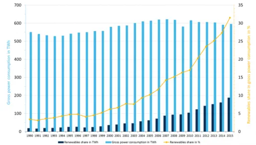
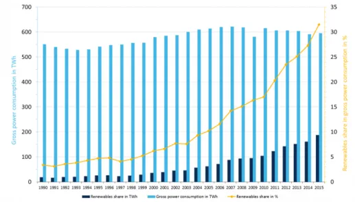
Conforme exposto na Figura 1.1, ocorreu um crescimento exponencial na capacidade de renov´aveis na Alemanha, em particular de paineis fotovoltaicos [3]. At´e 2010, cerca de metade de toda a energia FV gerada na Europa foi produzida na Alemanha, mas em virtude dos crescentes aumentos nos pre¸cos da energia e de pol´ıticas de incentivo `

a gera¸cão fotovoltaica adotadas por outros estados da União Européia, este percentual foi ligeiramente diminuido nos anos seguintes. Em 2015, as fontes renováveis supriram mais de 30 % do consumo de eletricidade na Alemanha.

(32)

Figura 1.1: Oferta de eletricidade e gera¸cão renovável alemã em TWh, entre 2001 e 2015. Fonte: [110], licen¸ca Creative Commons by SA 4.0.

De acordo com [52], no ano de 2014, a gera¸cão de eletricidade foi responsável por 23.815 TWh ou 18 % do consumo mundial de energia, partindo de 6.287 TWh ou 9.4 % em 1974. Combust´ıveis fósseis permanecem como a principal fonte primária da eletricidade, uma vez que óleo, carvão e gás natural são responsáveis por 66,7 % da gera¸cão, menor que os 75,2 % em 1974. Hidroelétrica é a maior fonte primária renovável, suprindo 16,4 % da gera¸cão em 2013, decaindo de 20,9 % em 1974. A participa¸cão da fissão nuclear triplicou entre 1974 e 2014, indo de 3,3 % para 10,6 % da gera¸cão. Todas as outras fontes combinadas, incluido solar e eólicas, foram em 2013 responsáveis por 6,3 % da gera¸cão.

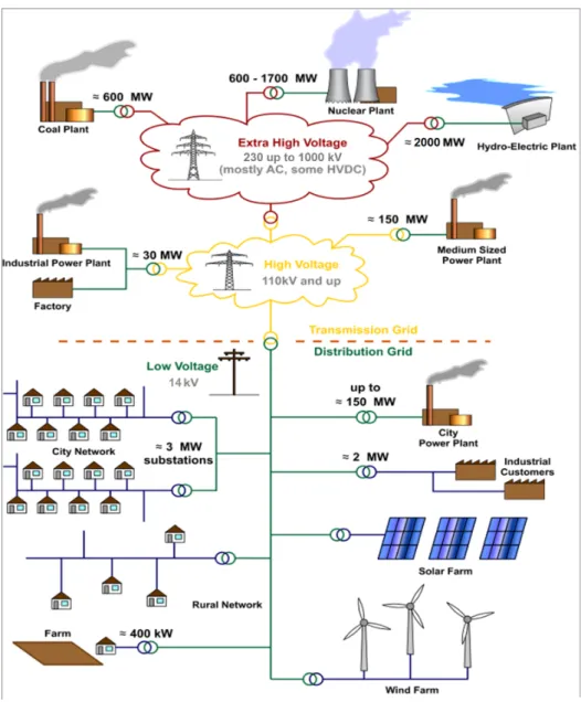
Um sistema elétrico é usualmente composto de três subsistemas: gera¸cão, transmissão e distribui¸cão. Gera¸cão representa a etapa de conversão da fonte primária de energia em eletricidade, usualmente realizada em grandes usinas localizadas a uma distância f´ısica considerável até os centros de carga. A transmissão é composta por linhas de alta tensão, projetadas para transportar eficientemente grandes blocos de eletricidade da gera¸cão até os sistemas de distribui¸cão. As redes de distribui¸cão são o último elo com os consumidores no setor elétrico, sendo este subsistema responsável por reduzir a tensão para os n´ıveis padronizados de consumo para fins industriais e residenciais, distribuindo eletricidade para um grande número de consumidores e garantindo que os padrões de qualidade de energia são atendidos.

(33)

Figura 1.2: Esquema simplificado de um sistema el´etrico com gera¸c˜ao distribu´ıda

Dado que o conjunto de requerimentos encontrados pelas companhias de distribui¸cão remontam a um cenário complexo, ferramentas robustas de previsão de demanda são necessárias para implementar planos de expansão e opera¸cões eficientes e razoáveis. Os sistemas elétricos atuais requerem um permanente equilibrio entre gera¸cão e carga, pois sistemas de armazenamento de energia em larga escala ainda não atingiram viabilidade econômica para a maioria das redes elétricas. Na ocorrência de um desequilibrio entre gera¸cão e demanda de energia, a frequência do sistema passa a oscilar e as unidades geradoras devem rapidamente aumentar ou diminuir a gera¸cão para se restabelecer o equilibrio e restaurar a estabilidade de frequência do sistema. A reserva girante de gera¸cão empregada para manter a estabilidade no presente é resultado do planejamento e da previsão de carga realizados no passado. Os planos de opera¸cão que determinam quando cada gerador permanece em modo de espera ou em gera¸cão nominal são também

(34)

oriundos de estudos de previs˜ao de demanda.

A inser¸cão de gera¸cão distribu´ıda adiciona um novo n´ıvel de complexidade a esta ta-refa, pois não somente a gera¸cão descentralizada reduz a carga de modo aleatório e intermitente, como também inevitavelmente produz altera¸cões nas séries históricas de carga usadas para fazer as previsões. Ambos efeitos agem no sentido de aumentar os erros de predi¸cão no curto e no longo prazo, amea¸cando a eficiência operacional e, no pior caso, a estabilidade do sistema [26].

Ao passo que todas as fontes de gera¸cão distribu´ıda tem visto crescimento na sua ca-pacidade instalada, a fonte solar fotovoltaica tem visto a maior taxa de implanta¸cão nos últimos anos. Nos Estados Unidos, Fotovoltaicas constituem de 80 a 90% da capa-cidade instalada dentre as instala¸cões de GD com até 2 MW. Na Alemanha, de acordo com [105], a energia fotovoltaica gerada somou 38,5 TWh e supriu aproximadamente 7,5 % do consumo l´ıquido de eletricidade da Alemanha em 2015, conforme ilustrado na figura 1.3. Em dias úteis ensolarados, a energia fotovoltaica pode atender 35 % da demanda instantânea, valor que sobe a 50 % em feriados e fins de semana. Ao fim de 2015, a capacidade nominal FV instalada na Alemanha foi de cerca de 40 GW distri-buidos em 1,5 milhão de unidades geradoras. Com este n´ıvel de grandeza, a capacidade instalada em FV excede a de todas as demais fontes na Alemanha.

Figura 1.3: Percentual de energia renov´avel no consumo l´ıquido de eletricidade na Alemanha, de 2005 a 2015. Em 2015 as fontes renov´aveis supriram 38 % do consumo. Fonte: [105]

Pa´ıses em desenvolvimento e emergentes tem também experimentado tendências se-melhantes. De acordo com a Agência Nacional de Energia Elétrica (ANEEL), desde a publica¸cão da Resolu¸cão Normativa 482/2012, tem havido um constante crescimento

(35)

no número de novas unidades de gera¸cão distribu´ıda conectadas à rede de distri-bui¸cão, conforme exposto na Figura 2.4. Esta Resolu¸cão Normativa regulamenta a conexão de gera¸cão distribu´ıda às redes de distribui¸cão, estabelecendo procedimentos e as obriga¸cões das empresas de distribui¸cão e dos consumidores.

Figura 1.4: Evolu¸cão trimestral do número de unidades de gera¸cão distribu´ıda conectadas às redes de distribui¸cão brasileiras. Fonte: ANEEL

Semelhantemente ao observado na Alemanha e nos Estados Unidos, a gera¸cão solar fotovoltaica é a maior fonte de gera¸cão distribu´ıda no Brasil, não somente em ca-pacidade instalada como particularmente no número de unidades conectadas. Esta predominância é mostrada na figura 1.5.

Figura 1.5: Capacidade instalada (esquerda) e n´umero de unidades conectadas (direita) no Brasil, divididas por fonte prim´aria de energia. Fonte: ANEEL

Este crescimento mundial da gera¸cão fotovoltaica é uma consequência da curva de aprendizado tecnológica e dos custos decrescentes, ilustrados na figura 2.6, que apre-senta os pre¸cos de mercado na Alemanha. A fonte fotovoltaica tem experimentado

(36)

r´apido desenvolvimento tanto em custo quanto em performance. Nos Estados Unidos, foi observado que os custos diminuiram 31 % de 2010 para 2014 [26], enquanto que na Alemanha os custos ca´ıram em quase 75 % desde 2006.

Figura 1.6: Custo médio l´ıquido do sistema FV para o consumidor, considerando sistemas para instala¸cão em telhados com potência nominal entre 10 kWp e 100 kWp. Fonte: [105]

Portanto, os operadores de sistemas de potência devem empregar ferramentas adaptati-vas que não somente são efetivas para prever a demanda, mas que também estão aptas a rastrear a mudan¸ca no comportamento da demanda ocasionado pela crescente pre-sen¸ca de GD. Por outro lado, os fatores relevantes que governam a gera¸cão fotovoltaica, como a irradia¸cão solar e a temperatura ambiente, são também correlacionados com o consumo de energia, embora de modo não linear. Aprimorando as metodologias de previsão para modelar e adaptar à presen¸ca de GD pode também melhorar ainda mais o desempenho destes métodos quando efetuando previsões em sistemas convencionais.

1.1 Formula¸c˜ao do problema

A previsão de carga é uma importante ferramenta empregada para assegurar que a energia suprida pelas distribuidoras está em equil´ıbrio com as cargas e com as perdas de energia inerentes ao sistema elétrico. A previsão de carga é sempre definida como a ciência ou arte de prever a carga futura em um dado sistema, por um per´ıodo de tempo determinado. Estas predi¸cões podem prever a carga para as horas e minutos seguintes, com o objetivo de auxiliar a opera¸cão, ou predizer a demanda a 20 anos

(37)

para fins de planejamento da expansão. A crescente capacidade instalada de recursos energéticos distribu´ıdos levanta novas questões para este campo de pesquisa, pois é necessário prever não apenas o crescimento da capacidade como também a gera¸cão intermitente associada à GD.

Com rela¸cão às escalas de tempo e ao alcance das predi¸cões, previsão de demanda pode ser categorizada em três áreas [90]:

1. Previsão de longo prazo, que é utilizada para predizer as cargas para até 50 anos no futuro, de modo que a suportar o planejamento para a expansão;

2. Previsão de médio prazo, que é utilizada para prever cargas semanais, mensais e anuais a até 10 anos no futuro, permitindo o planejamento eficiente das opera¸cões do sistema;

3. Previsão de curto prazo, que é empregada para prever cargas até uma semana no futuro, de modo a minimizar custos das opera¸cões diárias e despachos de gera¸cão.

Nas três categorias precedentes, um modelo acurado é necessário para representar ma-tematicamente a rela¸cão entre a carga e variáveis influentes, como datas, clima, fatores econômicos, entre outros. A rela¸cão precisa entre a carga e estas variáveis é usualmente determinada pelo seu papel no modelo de carga. Uma vez que este é constru´ıdo, os parâmetros do modelo são determinados por meio de técnicas de estima¸cão. Existem cinco componentes fundamentais em um problema de estima¸cão [90]:

1. As vari´aveis a serem estimadas

2. As medi¸c˜oes ou observa¸c˜oes dispon´ıveis

3. O modelo matemático que descreve como as medi¸cões estão relacionadas com a variável de interesse

4. O modelo matemático das incertezas de medi¸cão e estima¸cão

5. O critério de avalia¸cão de desempenho que irá julgar qual algoritmo é o “melhor”.

Nos últimos 50 anos, os algoritmos de estima¸cão de parâmetros usados na previsão de demanda limitaram-se à múltipla regressão baseada no critério de minimiza¸cão de

(38)

erro dos m´ınimos quadrados [47]. Estes métodos evoluiram para os de séries temporais estocásticas, a exemplo dos modelos Autorregressivos (AR) e de Médias Móveis (MA). Atualmente, o estado da arte reside em modelos de espa¸co de estados finamente ajus-tados e em sistemas especialistas, baseados em técnicas de aprendizado de máquina. Além disso, as Redes Neurais Artificiais (RNA) têm mostrado sucesso como a base de sistemas especialistas para a previsão de curto prazo. Contudo, o sistema especialista utilizado por uma empresa não necessariamente é adequado para o uso em um sistema elétrico diferente, no m´ınimo requerendo novo treinamento e algumas vezes a troca de variáveis ou do próprio modelo matemático para tornar-se útil para uma empresa diferente.

Este trabalho apresenta a previsão de carga e gera¸cão como um problema de estima¸cão dinâmica de estado. As variáveis a serem estimadas são as demandas base, média e de pico, assim como a gera¸cão fotovoltaica. Como medi¸cões e observa¸cões, este trabalho utiliza previsões de tempo, datas e eventos de calendário, tarifas de energia, ´ındices e estimativas econômicas e demográficas. Combina¸cões preprocessadas destas medi¸cões são usadas como as variáveis de entrada para a previsão. O modelo matemático é a representa¸cão em espa¸co de estados, e as matrizes de covariância do filtro de Kalman modelam as incertezas. Os critérios de performance incluem Erro Médio Quadrático (MSE), Erro Médio Percentual (MAPE) e Erro Máximo Percentual (MPE). Além des-tes, diferentes abordagens empregadas para solucionar este problema de estima¸cão dinâmica de estados são também discutidas, assim como são realizadas compara¸cões entre a solu¸cão propostas e outras solu¸cões do estado da arte.

A presente disserta¸cão contribui para este tópico de pesquisa ao propor e validar ferramentas de análise para produzir, aprimorar e selecionar conjuntos relevantes de variáveis de entrada, o que melhora a capacidade dos algoritmos de predi¸cão para pre-ver carga e gera¸cão fotovoltaica. Um esquema de predi¸cão h´ıbrido baseado em filtros de Kalman e modelos Grey é apresentado para com confiabilidade e precisão realizar a predi¸cão de carga e gera¸cão distribu´ıda. Como um resultado secundário, a modelagem de carga adotada neste trabalho pode ser empregada para sintetizar cargas estocásticas e geradores distribu´ıdos em sistemas elétricos simulados.

(39)

1.2 Organiza¸c˜ao da disserta¸c˜ao

Esta disserta¸cão está dividida em seis cap´ıtulos, bibliografia e quatro apêndices. Os cap´ıtulos apresentam os tópicos principais e as conclusões obtidas nesta pesquisa, en-quanto que a base matemática e os conceitos úteis que suportam as proposi¸cões deste trabalho estão organizados em apêndices.

O Cap´ıtulo 2 contém uma versão desta introdu¸cão em inglês, ao passo que este Cap´ıtulo 1 apresenta o mesmo conteúdo em lingua portuguesa.

O Cap´ıtulo 3 trata da modelagem da carga elétrica e da gera¸cão fotovoltaica que é desenvolvida neste trabalho. Premissas, suposi¸cões e conceitos aplicados ao longo deste trabalho para construir modelos razoáveis para cada tipo de carga e de gerador fotovoltaico podem ser encontrados neste cap´ıtulo. Também existe, para cada tipo de carga e gerador, uma discussão e os passos de preprocessamento necessários para produzir os fatores relevantes que devem ser inclu´ıdos como variáveis de entrada no algoritmo de predi¸cão.

O Cap´ıtulo 4 propõe um esquema adaptativo de predi¸cão para planejamento e opera¸cão de redes elétricas baseado em filtros de Kalman. Além do algor´ıtmo de predi¸cão, o cap´ıtulo também destaca o modelo de dados empregado, explicando a natureza e o preprocessamento das variáveis exógenas que são selecionadas como dados de entrada, assim como aborda o estado da arte em técnicas de predi¸cão de carga e de gera¸cão fotovoltaica.

O Cap´ıtulo 5 apresenta os resultados das previsões em diversos cenários. O algor´ıtmo de previsão de demanda é utilizado para predizer as cargas de base, média e de pico em dois sistemas elétricos distintos, um na Alemanha e outro no Brasil. A previsão de gera¸cão fotovoltaica é realizada em dois locais, na Holanda e na Nova Zelândia. Um comparativo é feito entre os algoritmos propostos e métodos do atual estado da arte.

O Cap´ıtulo 6 sumariza as realiza¸cões e constata¸cões obtidas por esta pesquisa, reali-zando uma conclusão objetiva a respeito dos algor´ıtmos de predi¸cão, os comparativos e as dire¸cões a serem tomadas em trabalhos subsequentes.

A bibliografia contém a listagem das referências bibliográficas que são citadas neste trabalho, organizadas em ordem alfabética.

(40)

O Apêndice A apresenta uma introdu¸cão para representa¸cões em espa¸co de estados e filtros de Kalman, também demonstrando o modelo espec´ıfico e a estrutura de filtro empregadas no método de previsão proposto. Apêndice B trata da modelagem da irradia¸cão solar e simula¸cão empregada tanto para prever a gera¸cão fotovoltaica quanto para aprimorar as previsões de demanda. Apêndice C fornece um sucinto fundamento a respeito de Análise de Componentes Principais, a principal ferramenta empregada para selecionar as variáveis de entrada para o algor´ıtmo proposto. O Apêndice D apresenta um resumo das técnicas de redes neurais artificiais usadas nesta pesquisa.

(41)

2 INTRODUCTION

Economic development, throughout the world, depends directly on the availability of electric energy, especially because most industries and basic services depend almost entirely on its use. The availability of a source of continuous, cheap, and reliable energy is of foremost economic importance.

Large amounts of energy supply are set apart worldwide to energetically intensive sectors such as water treatment, irrigation, transformation industry and transport. In particular, the richest countries have the highest energetic demands per inhabitant since Gross Domestic Product (GDP) is highly correlated with the energy demands.

This dependence can be linearly modeled considering data from 2003 to 2007 [2]. The causal relationship between economic growth, characterized in diverse indicators, and the electricity consumption is investigated in numerous of papers. The study presen-ted in [22] conclude that causality is stronger in developed OECD countries than in developing countries. Several variables are used to assert the dependencies between energy consumption and economic activities: Gross Domestic Product (GDP), popu-lation and price indexes [7]. In [11], Granger tests indicate short-run causality from energy consumption to income for India and Indonesia, while the test points to bidi-rectional relationship for Thailand and the Philippines. This bidibidi-rectional dependence points towards a feedback loop, where the availability of cheap energy supply promotes economic growth, and then the increased economic activity demands a even greater energy consumption and/or improved energy efficiency. From this standpoint, energy demands should be approached not only as a essential service, but also as an economic issue.

(42)

Table 2.1: Worldwide and Domestic German Energy Supply (DES), German Gross Domestic Product (GDP) and Population from 2000 to 2015

DES DES GDP Pop. DES / Capita

Year World Germany Germany Germany World — Germany (TWh) (TWh) 109_US$ ₁₀6_Inhab. _{TWh /10}6_Inhab.

2000 15406,03 579,6 1949,95 82,21 2,52 — 7,05 2001 15638,45 585,1 1950,65 82,35 2,52 — 7,11 2002 16190,43 587,4 2079,14 82,49 2,58 — 7,12 2003 16793,16 600,7 2505,73 82,53 2,64 — 7,28 2004 17572,76 610,2 2819,25 82,52 2,73 — 7,39 2005 18333,46 614,1 2861,41 82,47 2,81 — 7,45 2006 19030,16 619,8 3002,45 82,38 2,89 — 7,52 2007 19922,93 621,5 3439,95 82,27 2,98 — 7,55 2008 20283,94 618,2 3752,37 82,11 3,00 — 7,53 2009 20123,69 581,4 3418,01 81,90 2,94 — 7,10 2010 21404,5 615,0 3417,30 81,78 3,09 — 7,52 2011 22050,91 606,1 3757,46 81,80 3,15 — 7,41 2012 22504,33 605,7 3543,98 80,43 3,17 — 7,53 2013 23092,66 603,8 3752,51 82,13 3,22 — 7,35 2014 24240,89 591,1 3879,28 80,98 3,34 — 7,30 2015 25893,62 595,1 3363,45 81,41 3,52 — 7,31

The data in Table 2.1 extracted from [4, 3] shows the evolution of three indicators related to the world and the German economies over the period from 2000 to 2012. The first two columns in Table 2.1 correspond to the Domestic Energy Supply (DES) in the world and in Germany, respectively, while the third and fourth columns are the GDP and the population in millions of inhabitants in Germay. Finally, the last column in Table I presents DES/Capita for the World and Germany. Note that Ger-man population is practically constant although the amount of energy supplied has increased.

The energy consumption per inhabitant (DES/Capita) in Table 2.1follows an ascen-dant curve within 2000-2015, and that indicates the need for continuous investments in the electric grid. Load forecasting comes up, therefore, as an essential tool for the electricity distribution companies. Due to natural monopoly regulations enacted on

(43)

most countries, these companies must comply with several contractual standards re-lated to reliability, efficiency, safety and other power quality aspects. Moreover, the companies should equally take into account the scarcity and fluctuation of energy re-sources as much as environmental care such as CO2 emissions control [5]. Furthermore, the companies should also take heed of the increase on distributed generation on the demand side, mainly concerning photovoltaic generation, which is in rapid expansion throughout the world.

These are typically comprised of generation units rated from fractional kW and up to 5 MW in nameplate capacity, interconnected to the distribution system and installed either behind the consumer’s load or directly connected to the system, using the grid to provide power to a remote consumer unit. Solar photovoltaic systems transform solar energy into electric power. Semiconductors that exhibit the photovoltaic effect, such as silicon-N or silicon-P solar cells, convert solar radiation into Direct Current (DC) electricity. Solid state inverters then converts the DC generation into Alternate Current (AC), which is injected into the power grid.

As depicted in Fig. 2.1, there has been an exponential growth in the installed capacity of renewable sources in Germany, photovoltaic panels in particular [3]. Until 2010, over half of the entire PV generated power in Europe came out from Germany, but due to growing energy prices and PV friendly policies adopted by other EU states, this percentange has slightly decreased in the following years. In 2015, the renewable sources supplied more than 30 % of Germany’s electricity consumption.

Figure 2.1: German and European photovoltaic (PV) generated power in MW, between 2001 and 2015. Source: [110], Creative Commons license by SA 4.0.

(44)

According to the [52], in year 2014, the electricity generation accounted for 23,815 TWh or 18 % of the World total energy consumption, up from 6,287 TWh or 9.4 % in 1974. Fossil fuels are still the main primary source for electricity, as oil, coal and natural gas accounts for 66.7 % of the generation, down from 75.2 %. Hydropower is the main renewable source, supplying 16,4 % of the electricity generation in 2014, down from 20.9 %. Nuclear fission share has increased threefold between 1974 and 2014, from 3.3% to 10.6 % of the generation. The other sources combined, including solar and wind power, account for 6.3 % of the electricity production.

An electric system is usually composed of three subsystems: generation, transmission and distribution. Generation represents the conversion of a primary energy source into electricity, usually performed in large scale facilities at a considerable physical distance from the consumption centers. Transmission is comprised of high voltage power lines, designed to efficiently transport large blocks of electricity from generation to distri-bution facilities. Distridistri-bution grids are the last link to the consumers in the electric system, responsible to decreasing voltage for industrial and residential consumption and distributing the electricity to several consumers while ensuring that power quality standards are met.

Since the set of requirements faced by electricity distribution companies assemble a complex scenario, robust load forecasting tools are needed to implement efficient and reasonable expansion and operation plans. Current electric power systems require a permanent balance between generation and load, since large scale energy storage has not achieved economical feasibility in most power grids. At the onset of an unbalance between load and generation, the system frequency starts to oscillate and generation units must be quickly stepped up or down in order to reobtain balace and to restore the system’s frequency stability. The generation spinning reserve used to keep stability today is the result of planning and forecast performed several years prior. The opera-tional plans that determine when each generator stays at stand by or at full power is also a product of load forecasts.

The introduction of distributed generation adds a new level of complexity to this task, as not only the decentralized generation reduces load in a random and intermittent way, but also inevitably embeds in the historic loads used to forecast. Both effects act

(45)

Figure 2.2: Simplified schematic of a electric power system with Distributed Energy Resources

to increase prediction errors in short and long term, jeopardizing operational efficiency and, in worst case, system reliability [26].

While all DERs have seen growth in installed capacity, photovoltaic solar has seen the largest adoption in recent years. In the US, photovoltaic constitutes 80 to 90 % of the total installed capacity among DER installations two megawatts or less. In Germany, according to [105], photovoltaic generated power amounted to 38.5 TWh and covered approximately 7.5 % of Germany’s net electricity consumption in 2015, as depicted in Figure 2.3. On sunny weekdays, PV power can cover 35 percent of the momentary electricity demand, while on weekends and holidays the coverage rate of PV can reach 50 percent. At the end of 2015, the total nominal PV power installed in Germany was circa 40 GW, distributed over 1.5 million power plants. With this figure, the installed