Published online 17 December 2008 in Wiley InterScience (www.interscience.wiley.com) DOI: 10.1002/joc.1834
Trends in extreme precipitation indices derived from a daily
rainfall database for the South of Portugal
Ana Cristina Costa
a* and Am´ılcar Soares
baISEGI, Instituto Superior de Estat´ıstica e Gest˜ao de Informa¸c˜ao, Universidade Nova de Lisboa, Portugal bCERENA, Centro de Recursos Naturais e Ambiente, Instituto Superior T´ecnico, Portugal
ABSTRACT: The rainfall regime of the South of Portugal is Mediterranean with Atlantic influence. Long-term series of
reliable precipitation records are essential for land and water resources management, climate-change monitoring, modelling
of erosion and run-off, among other applications for ecosystem and hydrological impact modelling. This study provides a qualitative classification of 106 daily rainfall series from stations located in the South of Portugal and evaluates temporal patterns in extreme precipitation by calculating a number of indicators at stations with homogeneous data within the 1955/1999 period. The methodology includes both absolute and relative approaches and a new homogeneity testing procedure, besides the application of other statistical tests. The proposed technique is an extension of the Ellipse test that takes into account the contemporaneous relationship between several candidate series from the same climatic area (SUR+Ellipse test). The results indicate that this technique is a valuable tool for the detection of non-climatic irregularities in climate time series if the station network is dense enough. The existence of trends and other temporal patterns in extreme precipitation indices was investigated and uncertainty about rainfall patterns evolution was assessed. Three indices describing wet events and another three indicators characterizing dry conditions were analysed through regression models and smoothing techniques. The simple aridity intensity index (AII) reflects increases in the magnitude of dryness. Especially pronounced trends are found over most of southern Portugal in the 1955/1999 period, highlighting the fact that large areas are threatened by drought and desertification. The trend signals of the wetness indices are not significant at the majority of stations, but there is evidence of increasing short-term precipitation intensity over the region during the last three decades of the twentieth century. Finally, the results also indicate that extreme precipitation variability and climate uncertainty are greater in recent times. Copyright 2008 Royal Meteorological Society
KEY WORDS aridity; climate variability; extreme precipitation; homogeneity testing; Portugal; rainfall intensity; trend analysis Received 5 January 2008; Revised 6 November 2008; Accepted 11 November 2008
1. Introduction
Portugal is geographically located in the southwesterly extreme of the Iberian Peninsula (between 37° and 42°N and 6.5° and 9.5°W). Global circulation and regional climatic factors (e.g. latitude, orography, oceanic and continental influences) explain the spatial distribution of rainfall, as well as its intra-annual variability, i.e. seasonal variability (Trigo and DaCamara, 2000; Goodess and Jones, 2002). The precipitation regimes are of a different nature in northern and southern regions of Portugal: in the North the precipitation regime has an orographic origin, whereas in the South it is associated to cyclogenetic activity (Trigo and DaCamara, 2000). The inter-annual variability is of a different nature, since the circulation variability is insufficient to explain the observed inter-annual variability of rainfall (Trigo and DaCamara, 2000; Goodess and Jones, 2002; Haylock and Goodess, 2004). In southern Portugal, summer precipitation, almost close to zero during this season, is sometimes associated with * Correspondence to: Ana Cristina Costa, ISEGI, Universidade Nova de Lisboa, Campus de Campolide, 1070-312 Lisbon, Portugal. E-mail: ccosta@isegi.unl.pt
local convective activity. These storms can occur with a large degree of independence from the circulation weather type, which characterizes the Iberian circulation for that specific day (Trigo and DaCamara, 2000).
Recent studies, based on climate models and past observed records, predict a future increase in droughts in the South of Europe as a result of increased evapotranspi-ration and a relatively slow decrease of rainfall amounts and precipitation frequency (e.g. Kostopoulou and Jones, 2005; Vicente-Serrano and Cuadrat-Prats, 2007). The results obtained by Goodess and Jones (2002) for the Portuguese stations show general agreement with those from Trigo and DaCamara (2000) who considered ten classes of weather circulation types for Portugal. Their results suggest that the cyclonic class is associated with a fairly homogeneous distribution of precipitation over most of the country. Moreover, the ‘rainy’ classes with an Atlantic origin (mainly W and SW; NW to a lesser degree) are to be associated with the observed strong decrease in precipitation from North to South.
In arid and semi-arid regions such as the South of con-tinental Portugal, research on the extent of dryness and temporal trends in heavy rainfall events is an important
contribution to evaluate desertification dynamics and to identify areas potentially at risk from land degradation. However, studies focussing on the role of regional cli-mate change on erosivity and aridity factors are lacking for this region, especially at the local scale. This study attempts to compile a daily rainfall database for the South of Portugal and subsequently to evaluate temporal trends in extreme precipitation by calculating a number of cli-mate indices.
Besides the description of the study domain and pre-cipitation data, the first part of the article focuses on the detection of temporal discontinuities in the precipitation time series. This issue is of major importance, because non-climatic factors make data unrepresentative of the actual climate variation and might bias the studies’ con-clusions. A break could result from a recalibration of an instrument or a station relocation; a linear trend could result from a gradual but constant degradation of a sen-sor; and a non-linear trend could result from vegetative growth around the instruments. Several techniques have been developed for detecting inhomogeneities in time series of weather elements. The approaches underlying the homogenization techniques are quite different and typically depend on the type of element (temperature, precipitation, pressure, evaporation, etc.), the temporal resolution of the observations (annual, seasonal, monthly or sub-monthly), the availability of metadata (station’s history information) and the monitoring station network density (spatial resolution). A review of different meth-ods for the homogenization of climate series is presented by Peterson et al. (1998), and comparisons between pro-cedures are provided by Ducr´e-Robitaille et al. (2003) and Reeves et al. (2007). Following the hybrid approach proposed by Wijngaard et al. (2003) for the European Climate Assessment & Dataset (ECA&D) project, we did not attempt to remove non-climatic inhomogeneities from the 107 daily precipitation series compiled, but rather pro-vide a qualitative classification of each station’s records. Therefore, the results of the homogenization analysis were used to develop an overall classification of the daily series.
The second part of the article investigates the existence of trends and other temporal patterns in extreme precipi-tation indices, within the period 1955–1999, at 15 moni-toring stations located in southern Portugal. This 45-year period was chosen to optimize data availability across the region, taking into consideration the homogenization analysis performed. In all, three of the indices (SDII, R5D and R30) provide information on the ‘wetness’, whereas the other three [CDD, AII and frequency of dry spells (FDD)] characterize the ‘dryness’. The selected indices are appropriate for the purposes of this research, because they might contribute to assess climate dynamics that must be accounted for in impact studies related with water resources management, environmental policies, land use and desertification-related studies for the South of Por-tugal. The six daily precipitations indices were analysed through regression models and smoothing techniques.
This article is organized in two major parts. The first one (Section 2) addresses the homogenization assess-ment of the daily precipitation series, and the second part (Section 3) aims to characterize the dynamic tem-poral evolution of extreme precipitation indices in the 1955–1999 period. Finally, Section 4 states the major conclusions.
2. Daily rainfall database and quality control
2.1. Study domain and precipitation data
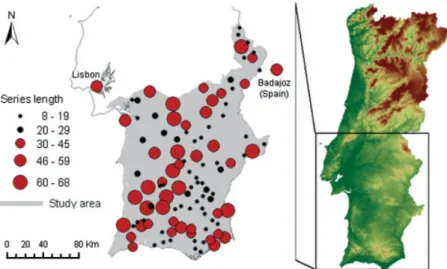
The study domain refers to the South of continental Portugal, and is defined by the Arade, Guadiana, Mira, Ribeiras do Algarve and Sado basins. The daily precipi-tation series analysed were compiled from the European climate assessment (ECA) dataset and the National Sys-tem of Water Resources Information (SisSys-tema Nacional de Informa¸c˜ao de Recursos H´ıdricos (SNIRH), man-aged by the Portuguese Institute for Water) database, and are available through free downloads from the ECA&D project website (http://eca.knmi.nl) and the SNIRH website (http://snirh.inag.pt), respectively. The analysed precipitation series were downloaded during the first semester of 2004. Despite being outside the study domain, data from Lisbon and Badajoz (Spain) stations were also compiled from the ECA dataset. All stations with at least 30 years with less than 5% of observa-tions missing were selected. Shorter series with at least 10 years lacking a maximum of 5% of data were also chosen, and hence the series with too many gaps were dis-carded. Using those criteria, 45 long-term and 62 short-term series of daily precipitation were accepted for the homogenization analysis. Even though the beginning and ending of series from the SNIRH database are highly variable, 44 long-term series have a common period of observation of 20 years, located in the 1964/1983 inter-val. Most of the long-term series (more than 90%) cover the standard normal period 1961/1990, and 33% of them extend back to 1931. Figure 1 shows the study domain and the geographical distribution of stations for which daily time series have been selected. The data are spa-tially representative of the study domain that covers approximately 25 200 km2.
Before being collected for this study, the daily series of the ECA dataset had already been subject to several basic quality-control procedures and statistical homogeneity testing. Because of the sparse density of the ECA station network, absolute tests were applied rather than rela-tive tests, i.e. testing candidate station’s series relarela-tive to neighbouring stations’ series, which are presumed homo-geneous. The ECA&D project used historic metadata information to find supporting evidence of changes in observational routines that may have triggered the irreg-ularities detected. The ECA daily series were not adjusted for the inhomogeneities identified. Instead, the results of the different tests were grouped in an overall classifica-tion (‘useful’, ‘doubtful’ and ‘suspect’). The four long-term precipitation series [Beja (666), Lisboa Geof´ısica
Figure 1. Study area and stations with daily precipitation series. Station dots are scaled with the length of the time series. Red dots: long-term series. Black dots: short-term series. This figure is available in colour online at www.interscience.wiley.com/ijoc
(675), Tavira (681) and Badajoz Talavera (709)] com-piled from the ECA dataset for this study were all marked as ‘useful’, as the four homogeneity tests did not reject the homogeneity hypothesis, at the 1% level (ECA&D project, http://eca.knmi.nl; Klein Tank et al., 2002; Wijn-gaard et al., 2003).
Some homogeneity testing of the annual precipitation totals of the stations from the SNIRH database has been carried out by Nicolau (1999), for the period 1959/1960–1990/1991. This author performed a double-mass analysis and three absolute homogeneity tests. Nicolau (1999) found no inhomogeneities in the annual precipitation series of the monitoring stations considered here. In summary, the full length of the series from the SNIRH database was not analysed and objective relative methods were not performed. Therefore, we assumed that the selected 107 daily precipitation series could contain potential breaks, as recommended by Auer et al. (2005), and thus several homogeneity testing procedures were applied to all of them.
2.2. Homogeneity assessment methodology
There are a number of tests available for the homoge-nization of climate series with low temporal resolution (e.g. Peterson et al., 1998). However, well-established statistical methods for the homogeneity testing of sub-monthly precipitation data are lacking (Wijngaard et al., 2003; Auer et al., 2005). Furthermore, adjusting daily and hourly data is not straightforward, thus the World Mete-orological Organization (WMO) makes no recommen-dations regarding adjusting sub-monthly data (Aguilar
et al., 2003). In order to overcome those limitations and
taking into consideration the previous quality control-analysis of the selected ECA series, the homogeneity assessment followed the hybrid approach proposed by Wijngaard et al. (2003) for the ECA dataset. Hence, the homogeneity procedures used as the testing variable, the annual wet day count with 1-mm threshold, which is expected to be representative of important characteristics of variation at the daily scale. The results of the different
procedures implemented were then used to develop an overall classification of the daily series.
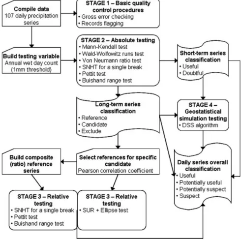
The homogeneity assessment of the precipitation time series was developed through four major stages (Figure 2). The first one comprises several basic qual-ity control-procedures that aim at the identification of errors and suspicious daily precipitation records, which were flagged using several criteria. The second stage is dedicated to absolute homogeneity testing and com-prises the application of six statistical tests to the test-ing variable, at all locations: the Mann–Kendall test (Mann, 1945; Kendall, 1975), the Wald–Wolfowitz runs test (Wald and Wolfowitz, 1943), the Von Neumann ratio test (Von Neumann, 1941), the Standard normal homo-geneity test (SNHT) for a single break (Alexandersson, 1986), the Pettit test (Pettit, 1979) and the Buishand range test (Buishand, 1982). In order to select a sub-set of series with quality data, the outcomes from the six tests were then grouped together, and a classification was established relying on the number of tests rejecting the homogeneity hypothesis at the 5% significance level. For the long-term series, the criteria were the follow-ing: (1) series considered homogeneous by all tests were classified as ‘reference’; (2) series for which only one of the six tests rejected the null hypothesis were clas-sified as ‘candidate’; (3) series for which two or more absolute tests rejected the homogeneity hypothesis were not analysed further. In the relative testing stage, the selected reference series were also tested through an iter-ative procedure in which they were seen consecutively as candidates and references. For the short-term series, two criteria were considered: (1) series considered homoge-neous by all tests were classified as ‘useful’; (2) series for which at least one of the absolute tests rejected the homogeneity hypothesis were classified as ‘doubtful’.
The relative testing stage comprises the application of those last three homogeneity tests to long-term compos-ite ratio series (Alexandersson and Moberg, 1997), and the application of a new procedure to the testing vari-able. This technique is an extension of the Ellipse test,
Figure 2. Schematic representation of the methodology for the homogeneity assessment of the precipitation time series. described by Allen et al. (1998), that takes into account
the contemporaneous relationship between several can-didate series from the same climatic area by using the residuals from a seemingly unrelated regression equations (SUR) model (Zellner, 1962), thus named SUR+ Ellipse test (Appendix).
Finally, in the fourth stage, a geostatistical stochastic simulation approach was applied to the testing variable of four candidate stations (Costa et al., 2008). This procedure uses the direct sequential simulation algorithm (Soares, 2001) to determine local probability density functions at candidate stations’ locations, by using spatial and temporal neighbouring observations. The results suggest that this procedure allows for the identification of breakpoints near the start and end of a series, and allows for the detection of multiple breaks simultaneously (Costa
et al., 2008). All other testing techniques considered were
used iteratively by systematically dividing the tested series into smaller segments when a break was detected, and then performing the test on those segments.
2.3. Homogeneity assessment results
All statistical tests results used the 5% significance level, and the data analysis was generated through specific programs developed using SAS software macros, SAS/STAT, SAS/ETS and SAS/GRAPH software of the SAS System (registered trademarks of SAS Institute Inc.) for Windows, Version 8.
2.3.1. Basic quality control analysis
Routine quality-control procedures revealed that all pre-cipitation records were non-negative but many series had non-existent dates, which were properly corrected and missing values were assigned to the variable for those days. Several robust location and scale estimates were computed for outlier detection by using all records from the daily time series, and by computing estimates for each year. The upper asymmetric pseudo-standard deviation (Lanzante, 1996) was computed for all 107 daily precip-itation series, but it was inconclusive since the median is equal to zero for all series and the third quartile is dif-ferent from zero for 11 series only, thus the interquartile range is always equal to zero except for those 11 series. The biweight estimates of the mean and standard devi-ation (Lanzante, 1996) could not be computed because the median-absolute-deviation (MAD) is equal to zero for all daily precipitation series and it appears in the weights denominator of those estimates. Similarly, Feng
et al. (2004) applied this procedure for temperature data
only. Robust alternatives to MAD are the Sn-and Qn
-standard deviations (Rousseeuw and Croux, 1993). The Sn-standard deviation is equal to zero for all daily
precip-itation series, and the Qn-standard deviation is
approxi-mately equal to 0.22 mm for all series, indicating that the centres of the distributions have low variability.
The next set of procedures aimed to identify ques-tionable data by flagging the daily precipitation records
with the following classification scheme: (1) ‘useful’, (2) ‘doubtful’, (3) ‘suspect’ and (4) ‘erroneous’. The first criterion relied on data outlying pre-fixed thresholds: records greater than the 99th percentile were flagged as (2); records greater than 100 mm were flagged as (3) and all others as (1). Using this criterion, 44% from the whole 107 series under analysis had records flagged as (3), in which 25 of them were long-term series and the other 22 were short-term series. Not surprisingly, the long-term series had an average number of records flagged as (3) approximately equal to 5, and for the short-term ones that average was approximately 3. The total number of records flagged as (3) was equal to 188. The second cri-terion used was a subjective evaluation of data previously flagged as (3), ‘suspect’. If at least two monitoring sta-tions had daily precipitation records greater than 100 mm on the same day, or within a 1-day range, their flag was set to (2), ‘doubtful’. As a result, the number of records flagged as (3) dropped to 52 and the number of series to 22 (16 long-term and 6 short-term).
The third criterion relied on graphical analysis. All 107 series were plotted against time, and when a peak in the graph seemed suspicious, even if that value was previously classified as (1) or (2), a closer look was taken by plotting the data against time together with highly correlated stations (Pearson’s correlation coeffi-cient greater than 0.70 or highly significant Spearman rank-order correlation coefficient) for the 3-month period centred in the suspicious day. After a subjective analysis of all the graphs (over 500), several records were reclas-sified. Afterwards, the Portuguese Institute for Water (INAG – Instituto da ´Agua) was contacted in order to clarify if data flagged as (4), ‘erroneous’ were outliers or a result of extreme weather phenomena. The erroneous values identified were then set to missing. Among the series with records flagged, the most problematic ones are Alcoutim (29M.01) and Picota (30K.02), both from the SNIRH database. It might be advisable to set to missing, the daily records of the years 1954–1959 of Alcoutim, as they were found highly suspicious. The daily precip-itation records of December 1972 and December 1973 are precisely the same in Picota, thus it might also be advisable to set them to missing.
The last quality-control procedure was a ‘flat line’ check (Feng et al., 2004), which identifies data of the same value for at least 3 consecutive days (not applied to zero precipitation data). For those detected records, the first occurrence was flagged as (0) ‘useful’, and the following records as (1) ‘suspect’. All other records were flagged as (0) ‘useful’. Almost half (49%) of the long-term series and 19% of the short-term ones were flagged with ‘suspect’ records using this methodology. The average number of runs (blocks of 3 or 4 consecutive days having the same value) per station was equal to two. The flagged precipitation values range from 0.1 to 5 mm and the most common values were 0.1 and 0.2 mm. This seems to indicate that if those flagged values are erroneous they might have been originated by measurement errors (i.e. how precisely very low amounts
of precipitation are measured) rather than by editing errors.
2.3.2. Absolute testing
The absolute testing stage comprises the application of six statistical tests to the testing variable at the 107 monitoring stations. Two of the homogeneity tests applied are not distribution free, namely the SNHT and the Buishand range test, and assume that data are independent, identically normally distributed random quantities. Moreover, the remaining non-parametric tests applied also require serially independent data. For those reasons, generalized Durbin–Watson autocorrelation tests and four normality tests were applied to the testing variable series at all stations.
The Durbin–Watson test is a widely used method of testing for autocorrelation. The generalized Durbin– Watson statistics for 1st, 2nd and 3rd order autocorrela-tion were computed, and conclusions were drawn at the 5% level. The generalized Durbin–Watson tests revealed 1st-order autocorrelation for almost 19% of the series (16 long-term and 4 short-term), and 2nd-order for four series only. None of the testing series had significant 3rd-order autocorrelation. The four normality tests applied were the Shapiro–Wilk, the Kolmogorov–Smirnov, the Cram´er–von Mises and the Anderson–Darling tests. For details on the statistical computation of the normality tests refer to SAS Institute (1999, pp. 1397–1401). In view of the results from those four normality tests, over 80% of the testing series (36 long-term and 50 short-term) were considered as Gaussian by all of them. On the other hand, the four tests rejected the normality hypothesis for 7.5% of the series (2 long-term and 6 short-term). Taking into consideration these results, we decided to proceed with the homogeneity tests. Moreover, it is a standard procedure to relax those assumptions for annual data.
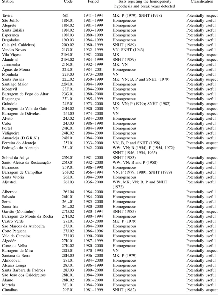
Regarding the homogeneity testing results (Table I), approximately 38% of the long-term series were consid-ered appropriate to be selected as reference, and 24% as candidate. Thus, the remaining 38% were excluded from the relative testing analysis. Not surprisingly, approx-imately 76% of the short-term series were considered homogeneous by the six statistical tests, and thus globally evaluated as ‘useful’.
2.3.3. Relative testing
The results from the relative testing stage are detailed in Table II. The series from Viana do Alentejo (24I.01) were not tested using the SUR+ Ellipse test because it was not possible to determine a common period, without too many gaps, for all the series that would be appropriate to model simultaneously (candidates and their respective references). All the regressors (reference series) parame-ters of the SUR models are statistically significant. Each SUR model includes at least two candidate stations’ data, and some series were tested more than once through dif-ferent models, depending on the common period of the
Table I. Results from the absolute testing stage and overall classification of the daily series. The Mann – Kendall (MK), Wald – Wolfowitz (WW), Von Neumann (VN), SNHT, Pettit (P) and Buishand (B) tests were applied to the annual number
of wet days (threshold 1 mm), and used the 5% significance level.
Station Code Period Tests rejecting the homogeneity
hypothesis and break years detected
Classification
Tavira 681 1941 – 1994 MK; P (1979); SNHT (1978) Potentially suspect
S˜ao Juli˜ao 18N.01 1981 – 1999 Homogeneous Potentially useful
Alegrete 18N.02 1981 – 1999 Homogeneous Potentially useful
Santa Eul´alia 19N.02 1983 – 1999 Homogeneous Potentially useful
Esperan¸ca 19N.03 1980 – 1999 Homogeneous Potentially useful
Degolados 19O.03 1984 – 1999 Homogeneous Potentially useful
Caia (M. Caldeiras) 20O.02 1980 – 1999 SNHT (1989) Potentially useful
Vendas Novas 21G.01 1932 – 1999 VN; SNHT (1943) Potentially useful
Vila Vi¸cosa 21M.01 1981 – 2000 MK Potentially suspect
Alandroal 21M.02 1984 – 1999 SNHT (1989) Potentially suspect
Juromenha 21N.01 1932 – 1999 MK; VN Potentially useful
´
Aguas de Moura 22E.01 1984 – 2001 Homogeneous Potentially useful
Moinhola 22F.03 1973 – 2000 VN Potentially useful
Santa Susana 22L.02 1950 – 1999 MK; VN; B, P and SNHT (1979) Potentially suspect
Santiago Maior 22M.01 1984 – 1999 Homogeneous Potentially useful
Montevil 23F.01 1984 – 2000 Homogeneous Potentially useful
Barragem de Pego do Altar 23G.01 1980 – 2000 Homogeneous Potentially useful
Reguengos 23L.01 1985 – 1999 Homogeneous Potentially useful
Grˆandola 24F.01 1973 – 2000 MK; VN; P (1979); SNHT (1982) Potentially suspect
Barragem do Vale do Gaio 24H.02 1980 – 2000 VN Potentially suspect
Barragem de Odivelas 24I.03 1974 – 2000 VN Potentially suspect
Alvito 24J.02 1984 – 2000 Homogeneous Potentially useful
Cuba 24J.03 1986 – 1998 Homogeneous Potentially useful
Portel 24K.01 1984 – 1999 Homogeneous Potentially useful
Vidigueira 24K.02 1984 – 2000 Homogeneous Potentially useful
Amareleja (D.G.R.N.) 24N.01 1984 –2000 Homogeneous Potentially useful
Ferreira do Alentejo 25I.01 1933 – 2000 VN; B, P and SNHT (1958) Potentially suspect Pedrog˜ao do Alentejo 25L.01 1942 – 2000 WW; VN; B (1954); P (1954, 1972);
SNHT (1946, 1954, 1965)
Potentially suspect
Sobral da Adi¸ca 25N.01 1981 – 2000 SNHT (1983) Potentially suspect
Santo Aleixo da Restaura¸c˜ao 25O.01 1932 – 2000 WW; VN; B and P (1958) Potentially useful
Barrancos 25P.01 1986 – 1998 Homogeneous Potentially useful
Barragem de Campilhas 26F.02 1956 – 1994 VN; P (1979, 1989); SNHT (1979) Potentially useful
Santa Vit´oria 26I.01 1984 – 2000 Homogeneous Potentially useful
Aljustrel 26I.03 1936 – 2000 WW; MK; VN; B, P and SNHT
(1972)
Potentially useful
Albernoa 26J.04 1984 – 2000 Homogeneous Potentially useful
Salvada 26K.01 1984 – 2000 Homogeneous Potentially useful
Serpa 26L.01 1985 – 2000 Homogeneous Potentially useful
Santa Iria 26L.02 1980 – 2000 Homogeneous Potentially useful
Garv˜ao (Montinho) 27G.02 1980 – 1994 SNHT (1983) Potentially suspect
Barragem do Monte da Rocha 27H.02 1980 – 1994 Homogeneous Potentially useful
Castro Verde 27I.01 1932 – 2000 MK; P (1979) Potentially useful
S˜ao Marcos da Ataboeira 27J.01 1984 – 2000 Homogeneous Potentially useful
Corte Pequena 27J.02 1986 – 1996 Homogeneous Potentially useful
Vale de Camelos 27J.03 1990 – 2000 Homogeneous Potentially useful
Algodˆor 27K.01 1987 – 1999 Homogeneous Potentially useful
Corte da Velha 27K.02 1980 – 2000 Homogeneous Potentially useful
Barragem de Mira 28G.01 1970 – 1993 VN Potentially suspect
Santana da Serra 28H.03 1936 – 2000 MK; P (1979) Potentially useful
Almodˆovar 28I.01 1984 – 2000 Homogeneous Potentially useful
Alcaria Longa 28J.01 1986 – 1999 Homogeneous Potentially useful
Santa Barbara de Padr˜oes 28J.03 1980 – 2000 Homogeneous Potentially useful S˜ao Jo˜ao dos Caldeireiros 28K.01 1984 – 2000 Homogeneous Potentially useful
´
Alamo 28K.02 1981 – 2000 Homogeneous Potentially useful
M´ertola 28L.01 1984 – 2000 Homogeneous Potentially useful
Table I. (Continued ).
Station Code Period Tests rejecting the homogeneity
hypothesis and break years detected
Classification
Foz do Farelo 29F.02 1981 – 1999 SNHT (1983) Potentially suspect
S˜ao Barnab´e 29I.01 1965 – 2000 VN; P (1972) Potentially suspect
Santa Clara-a-Nova 29I.02 1981 – 1999 Homogeneous Potentially useful
Guedelhas 29J.05 1980 – 1999 Homogeneous Potentially useful
Martim Longo 29K.01 1985 – 2000 Homogeneous Potentially useful
Malfrades 29K.03 1981 – 1999 Homogeneous Potentially useful
Penedos 29K.04 1981 – 2000 MK; SNHT (1995) Potentially useful
Pereiro 29L.01 1958 – 1999 VN; B (1983); SNHT (1995) Potentially suspect
Monte dos Fortes 29L.03 1984 – 1999 Homogeneous Potentially useful
Alcoutim 29M.01 1939 – 1999 WW; VN; B, P and SNHT (1959) Potentially suspect
Marmelete 30E.02 1984 – 1999 Homogeneous Potentially useful
Monchique 30F.01 1933 – 1998 WW; VN Potentially useful
S˜ao Bartolomeu de Messines 30H.03 1991 – 1998 Homogeneous Potentially useful
Paderne 30H.05 1984 – 1999 MK Potentially suspect
Sobreira 30I.02 1943 – 1999 WW; VN; B (1954); SNHT (1949) Potentially useful
Mercador 30K.01 1984 – 1999 Homogeneous Potentially useful
Faz-Fato 30L.03 1956 – 1999 VN; B and P (1986) Potentially suspect
Lagos 31E.01 1956 – 1999 MK; B and SNHT (1972); P (1979) Potentially suspect
Porches 31G.02 1980 – 1998 Homogeneous Potentially useful
Algoz 31H.02 1981 – 1996 Homogeneous Potentially useful
S˜ao Br´as de Alportel 31J.01 1985 – 2000 Homogeneous Potentially useful
Estoi 31J.04 1984 – 1999 Homogeneous Potentially useful
Santa Catarina (Tavira) 31K.01 1984 – 1999 Homogeneous Potentially useful
Quelfes 31K.02 1982 – 1998 Homogeneous Potentially useful
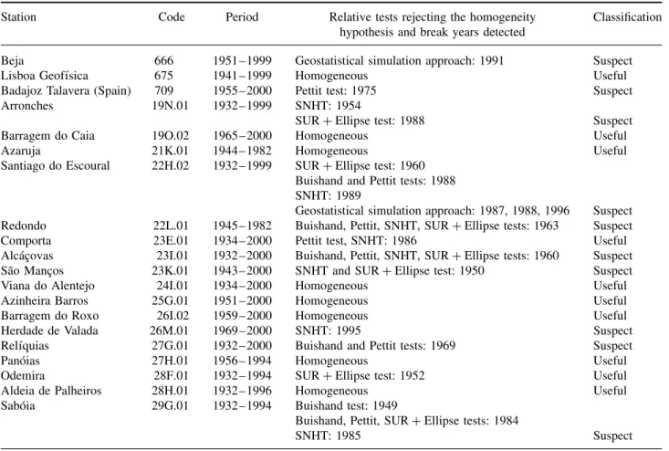
Table II. Results from the relative testing stage and overall classification of the daily series. The Buishand, Pettit, and SNHT tests were applied to composite (ratio) reference series. The SUR+ Ellipse test and the geostatistical simulation approach (Costa
et al., 2008) were applied to the annual number of wet days (threshold 1 mm). All tests used the 5% significance level.
Station Code Period Relative tests rejecting the homogeneity
hypothesis and break years detected
Classification
Beja 666 1951 – 1999 Geostatistical simulation approach: 1991 Suspect
Lisboa Geof´ısica 675 1941 – 1999 Homogeneous Useful
Badajoz Talavera (Spain) 709 1955 – 2000 Pettit test: 1975 Suspect
Arronches 19N.01 1932 – 1999 SNHT: 1954
SUR+ Ellipse test: 1988 Suspect
Barragem do Caia 19O.02 1965 – 2000 Homogeneous Useful
Azaruja 21K.01 1944 – 1982 Homogeneous Useful
Santiago do Escoural 22H.02 1932 – 1999 SUR+ Ellipse test: 1960 Buishand and Pettit tests: 1988 SNHT: 1989
Geostatistical simulation approach: 1987, 1988, 1996 Suspect Redondo 22L.01 1945 – 1982 Buishand, Pettit, SNHT, SUR+ Ellipse tests: 1963 Suspect
Comporta 23E.01 1934 – 2000 Pettit test, SNHT: 1986 Useful
Alc´a¸covas 23I.01 1932 – 2000 Buishand, Pettit, SNHT, SUR+ Ellipse tests: 1960 Suspect S˜ao Man¸cos 23K.01 1943 – 2000 SNHT and SUR+ Ellipse test: 1950 Suspect
Viana do Alentejo 24I.01 1934 – 2000 Homogeneous Useful
Azinheira Barros 25G.01 1951 – 2000 Homogeneous Useful
Barragem do Roxo 26I.02 1959 – 2000 Homogeneous Useful
Herdade de Valada 26M.01 1969 – 2000 SNHT: 1995 Suspect
Rel´ıquias 27G.01 1932 – 2000 Buishand and Pettit tests: 1969 Suspect
Pan´oias 27H.01 1956 – 1994 Homogeneous Useful
Odemira 28F.01 1932 – 1994 SUR+ Ellipse test: 1952 Useful
Aldeia de Palheiros 28H.01 1932 – 1996 Homogeneous Useful
Sab´oia 29G.01 1932 – 1994 Buishand test: 1949
Buishand, Pettit, SUR+ Ellipse tests: 1984
Table II. (Continued ).
Station Code Period Relative tests rejecting the homogeneity
hypothesis and break years detected
Classification
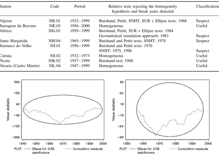
Aljezur 30E.01 1932 – 1999 Buishand, Pettit, SNHT, SUR+ Ellipse tests: 1968 Suspect
Barragem da Bravura 30E.03 1956 – 2000 Homogeneous Useful
Alferce 30G.01 1959 – 1999 Buishand, Pettit, SUR+ Ellipse tests: 1984
Geostatistical simulation approach: 1983 Suspect Santa Margarida 30H.04 1965 – 1999 Buishand and Pettit tests, SNHT: 1978 Suspect Barranco do Velho 30J.01 1956 – 1999 Buishand and Pettit tests: 1976
SNHT: 1975, 1996 Suspect
Catraia 30J.02 1932 – 1973 Homogeneous Useful
Picota 30K.02 1957 – 1999 Buishand test: 1988 Useful
Alcaria (Castro Marim) 30L.04 1947 – 1999 Homogeneous Useful
Figure 3. SUR+ Ellipse test results for the annual number of wet days (threshold 1 mm) at Aljezur (30E.01) station (left graph: testing period is 1941/99; right graph: testing period is 1956/97).
series included in each model. Consequently, depend-ing on the testdepend-ing period, different models sometimes provided different results for a specific candidate series. This problem can be minimized by testing the candidate series through a different model whenever a peak in the graph from the Ellipse test seems suspicious (Figure 3, left graph), or by using a combination of statistical tests. In fact, Wijngaard et al. (2003) state that, generally, a combination of statistical methods and methods relying on metadata information is considered to be most effec-tive to track down inhomogeneities. Nevertheless, that problem might also happen with other testing methods, although it is harder to detect because the tests are usu-ally applied only once. For example, applying the SNHT to the testing variable of Vendas Novas (21G.01) station for the period 1932/1992 concludes the series as homoge-neous, but testing the period 1938/1999 identifies a break in 1943.
The relative magnitudes of the breaks detected are given by the ratio between the average annual wet day count before and after two consecutive breaks. The magnitudes of the breaks detected by the SUR+ Ellipse test, but not identified by the other methods, range from −7.6% to 6.88%. Conversely, the magnitudes of the breaks detected by at least one of the other three
tests, but not identified by the SUR+ Ellipse test range from −14.09 to 10.78%. Hence, there is no apparent connection between the potential breaks magnitudes and the ability of the SUR+ Ellipse test to identify them.
Only 4 of the 11 series previously classified as candi-dates were considered as homogeneous by all the relative tests. Considering the 17 series previously classified as references, 8 of them were considered as homogeneous by all the relative tests. The breaks detected are mainly located between 1949 and 1954, and around 1986. There-fore, there is an apparent trend towards less breaks in recent times, in contrast to that reported by other homog-enization studies (Tuomenvirta, 2001; Wijngaard et al., 2003; Auer et al., 2005). The station selection was on the basis of the absolute testing results, thus that appar-ent trend may not be true if all the 107 stations’ series were tested through the relative approach.
2.3.4. Overall classification and discussion
An overall classification of the daily precipitation series was established using four classes (Table III): ‘use-ful’, ‘potentially use‘use-ful’, ‘potentially suspect’ and ‘sus-pect’. A series was classified as ‘useful’ when all rel-ative approaches (the four relrel-ative statistical tests and the stochastic approach) considered it as homogeneous.
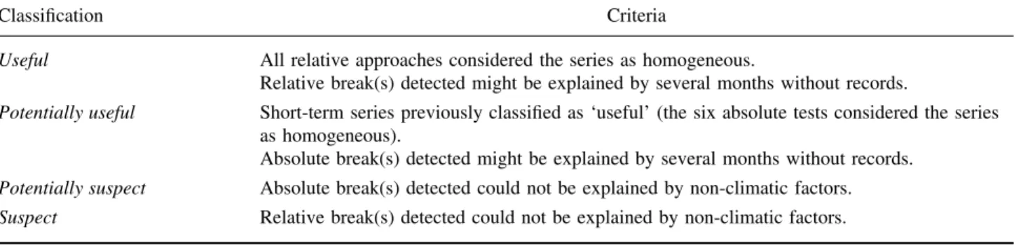
Table III. Criteria used to establish the overall classification of the daily series.
Classification Criteria
Useful All relative approaches considered the series as homogeneous.
Relative break(s) detected might be explained by several months without records.
Potentially useful Short-term series previously classified as ‘useful’ (the six absolute tests considered the series as homogeneous).
Absolute break(s) detected might be explained by several months without records.
Potentially suspect Absolute break(s) detected could not be explained by non-climatic factors.
Suspect Relative break(s) detected could not be explained by non-climatic factors.
Whenever the daily series had several months without records near a break year, identified by some relative test-ing procedure, the series was also classified as ‘useful’, because it is conceivable that the inhomogeneous records were set to missing in the SNIRH database, and the tests rejections were due to them. A series was classified as ‘suspect’ when at least one of the relative approaches considered it as inhomogeneous and the break(s) detected could not be explained by non-climatic factors.
Considering the series analysed through absolute test-ing only (both short and long-term), it is difficult to determine if changes or lack of changes result from non-climatic or non-climatic influences (Peterson et al., 1998), since it was not possible to find historic metadata support. Therefore, the intermediate classes, ‘potentially useful’ and ‘potentially suspect’, were established. Furthermore, as the short-term series were only analysed through abso-lute testing, those series were classified as ‘potentially useful’ if the six absolute tests considered the series as homogeneous. Relative approaches that use data from ref-erence stations are usually preferred because they aim to isolate the effects of station irregularities and to account for regional climate changes. In fact, the results show that the relative tests identified inhomogeneities in a number of stations that were previously considered as homoge-neous by the six absolute tests, and vice-versa. Although desirable, a relative approach for the homogeneity assess-ment of all series could not be used since it was out of the scope of this research.
Following those criteria, approximately 13% of the 107 series were classified as ‘useful’, 55% were classified as ‘potentially useful’, 19% were classified as ‘potentially suspect’ and 13% as ‘suspect’ (Tables I and II). Although defined with different criteria, the qualitative interpreta-tion of the overall classes is similar to the one given for the categories defined for the ECA series (Wijngaard
et al., 2003). However, it is important to point out that
we used the 5% significance level in all statistical tests, whereas those authors used the 1% level. Therefore, our classification is more conservative in the sense that we allowed for the rejection of the homogeneity hypothesis at stations that are considered homogeneous at the 1% significance level. The series classified as ‘useful’ seem to be sufficiently homogeneous for trend analysis and variability analysis. The series classified as ‘potentially
useful’ and ‘potentially suspect’ should be used cau-tiously, from the perspective of the existence of possible inhomogeneities, as the homogeneity analysis performed might be considered inconclusive – even though all series were considered homogeneous by previous studies. The series classified as ‘suspect’ should be excluded from trend analysis and variability analysis, as there is strong evidence of inhomogeneities present.
3. Trends in indices of daily extreme precipitation
Numerous extreme precipitation indices are described and analysed in the literature (Peterson et al., 2001; Frich
et al., 2002; Kiktev et al., 2003; Klein Tank and K¨onnen,
2003; Haylock and Goodess, 2004; Kostopoulou and Jones, 2005; Moberg and Jones, 2005). There are two main categories of extremes indices: those based on either absolute thresholds or percentiles. The first category refers to counts of days crossing a specified absolute value (e.g. the number of days per year with daily precipitation exceeding 30 mm). The second category of indices is on the basis of statistical quantities such as percentiles, so the tails of the statistical distribution are examined and days exceeding (not exceeding) a given high (low) percentile are counted. Indices based on percentile thresholds have a clear advantage for climate-change detection studies as they compare the climate-changes in the same parts of the precipitation distributions and thus can be used in studies of wide regions (Haylock and Nicholls, 2000; Klein Tank and K¨onnen, 2003). On the other hand, indices based on the count of days crossing certain fixed thresholds are beneficial for impact studies as they can be related with extreme events that affect human society and the natural environment (Klein Tank and K¨onnen, 2003).
The later set of indices, and indices describing events with short return periods (moderate climate extremes), are suitable for the purposes of this research since they might contribute to assess climate dynamics at the local scale that contribute for land degradation and desertifica-tion prone areas of the South of Portugal. Accordingly, we selected four extreme precipitation indices recom-mended by the joint CCI/CLIVAR/JCOMM Expert Team on Climate Change-Detection and Indices (ETCCDI, http://www.clivar.org/organization/etccdi/etccdi.php; Peterson et al., 2001; Frich et al., 2002), and developed
two other indices describing dry conditions. The follow-ing sections explain the criteria for station selection from the developed daily rainfall database, the indices ratio-nale and definitions, the trend analysis methodology and, in the last section, the results are summarized and dis-cussed.
3.1. Analysis period and data selection
From the set of 107 stations compiled for homogeneity assessment, one station’s data (29G.01 Sab´oia) were excluded from the analysis because multiple breakpoints were identified and the homogeneous periods were too short and unreliable; the Badajoz Talavera (709) station, in Spain, was also excluded. The daily rainfall database for the South of Portugal comprises records in the period 1931/2000, but the beginning and ending of each series are highly variable. The selection of stations with quality data for a long common period was developed through several stages.
First, the extreme precipitation indices were computed for the set of 105 stations, regardless of their overall homogeneity classification. Nevertheless, only the longest homogeneous period was used to build the indices for the series classified as ‘suspect’. The extreme precipitation indices are sensitive to the number of missing days, thus the daily records of the selected stations should be as complete as possible. Consequently, for each station, the indices for a specific year were set to missing if there were more than 16% of the days missing for that year (Haylock and Goodess, 2004).
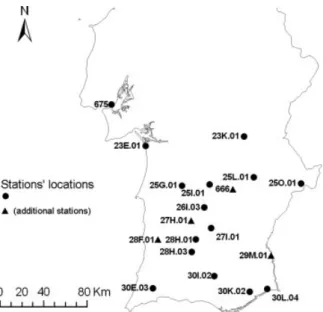
Next, a first set of stations was selected for trend anal-ysis by including all the series classified as ‘potentially useful’, ‘useful’ and the longest homogeneous period of the series classified as ‘suspect’. In this set, the number of stations with at least 30 years of overlapping observations was very small. Hence, the next stage aimed to select sta-tions classified as ‘potentially suspect’ with break years near the beginning of the series (identified through abso-lute testing), so that their longest homogeneous period could also be considered. This allowed us to determine the analysis period 1955/1999, which is the longest com-mon period for the final set of 15 series. The regional analysis of anomalies used four additional series with homogeneous records within 1940/2000 (Figure 4). All stations selected have less than 12% of the days missing in each year, and the data for most stations do not have any missing records.
3.2. Precipitation indices
In the present study only annually specified indices are considered. Their definitions are listed in Table IV. The SDII is a simple daily intensity index defined as the average precipitation per wet day and a wet day is defined as a day with at least 1 mm of precipitation. The R5D index is defined as the highest consecutive 5-day precipitation total and can be considered a flood indicator, since it provides a measure of short-term precipitation intensity. The R30 index characterizes the frequency
Figure 4. Stations selected for trend analysis. Dots: stations with nearly complete records in 1955–1999. Triangles: additional stations with data within 1940–2000 used to build the regional-average anomaly time
series.
of extremely heavy precipitation events and is defined as the number of days with daily precipitation totals above or equal to 30 mm. This threshold fits the extreme events regime of the study area as the 30-mm value approximately corresponds to the 95% regional-average percentile of the 1961/90 climate normal. The CDD index corresponds to the maximum number of consecutive dry days, and therefore characterizes the length of the greatest dry spell.
Not only drought but also moderate dry conditions have significant impacts in terms of crop losses, water supply shortages, land degradation and desertification in the South of Portugal. To better understand the pluviometric regime of this region, and the frequency and magnitude of dryness in particular, we developed two indices describing dry events (FDD and AII).
The FDD index is defined as the number of dry spells. For return periods of 2 years, expected dry-lengths vary from 60 to 80 days in the study region (Lana
et al., 2008). The selected indices refer to precipitation
events with return periods typically of less than 1 year, providing relevant information to impact studies. In the FDD definition, a dry spell is a consecutive period with at least 8 dry days. The average length of dry spells in a year ranges from 8 to 12 days in the study region (Lana
et al., 2008). Therefore, increasing (decreasing) trends of
FDD are indicators of a change in the mean frequency of dry events, rather than in the frequency of extremely dry situations,although a change in the extreme values of the distribution obviously implies a change in the mean.
Regarding the SDII, CDD and FDD indices, a wet day is defined as a day with at least 1 mm of precipitation (R ≥1 mm), thus a dry day has less than 1 mm of precipitation (R <1 mm). Ceballos et al. (2004) state that rainfall amounts below this threshold are not absorbed by soils and are evaporated off directly. In fact, Moberg and
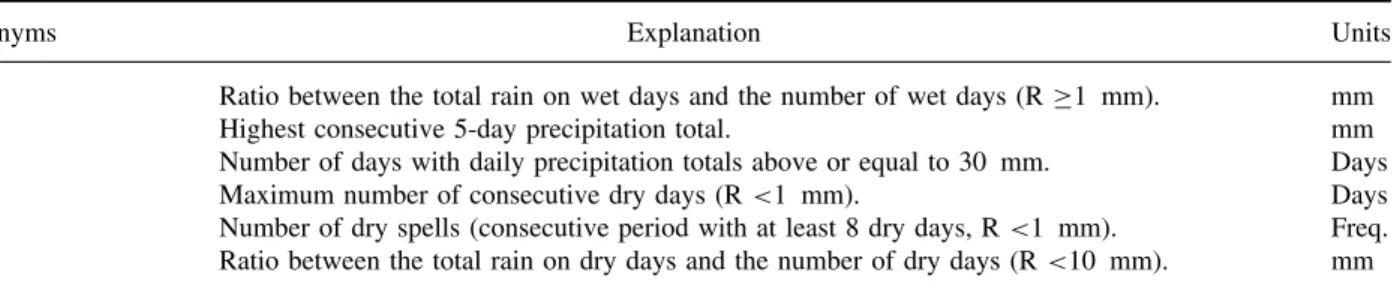
Table IV. Acronyms and definitions of the six indices for moderate precipitation extremes.
Acronyms Explanation Units
SDII Ratio between the total rain on wet days and the number of wet days (R≥1 mm). mm
R5D Highest consecutive 5-day precipitation total. mm
R30 Number of days with daily precipitation totals above or equal to 30 mm. Days
CDD Maximum number of consecutive dry days (R <1 mm). Days
FDD Number of dry spells (consecutive period with at least 8 dry days, R <1 mm). Freq. AII Ratio between the total rain on dry days and the number of dry days (R <10 mm). mm
Jones (2005) agree that, with this definition, a dry day is allowed to have a small amount of precipitation, but generally small enough as the ground will not recover after a long period of dryness. Moreover, thresholds lower than 1 mm can introduce trends in the number of wet days, associated with measurement errors introduced by the observers (Haylock and Nicholls, 2000; Haylock and Goodess, 2004) or by instrument inaccuracies. In fact, taking into consideration the ‘flat line’ check results, it is prudent to adopt such a threshold for dry days (R
<1 mm) because it allows for minimizing any inaccuracy associated with measurement errors.
In the definition of the AII index, we used the 10-mm threshold to indicate a dry day (Ceballos et al., 2004; Lana et al., 2008). Let RL10t be the total rain on days with precipitation amount below 10 mm (R
<10 mm), and let RL10 be the number of days with R <10 mm. Similar to the SDII, the AII index is defined by RL10t/RL10 and can be interpreted as a simple aridity index, because it is a numerical indicator of the degree of dryness of the climate at a given location. Below the 10-mm threshold, the rainfall has a small effect on the soil water-content, since the rainfall evaporates very quickly and hardly drains into the upper soil layer (Ceballos et al., 2004). Increasing (decreasing) trends of AII are indicators of change in the normal moisture availability, which is a sensitive issue for desertification susceptible regions. 3.3. Trend estimation and diagnosis methods
The six daily precipitations indices were subject to a number of diagnosis tests, at each station’s location, in order to verify the existence of autocorrelation and het-eroscedasticity of the regression errors. Depending on the tests’ results, the trend estimation was performed using three different regression models. The indices are expressed as annual values Yt, t = 1 , . . . , T with the sub-script t referring to the year (also denoted by Xt), and
T is the length of the period covered by the station’s series. Engle’s Lagrange multiplier test for heteroscedas-ticity (Engle, 1982) allows to test if the regression errors variance has the form V (εt)= σt2= α1+ α2Xt, where
εt is the disturbance term (error) of the ordinary least squares (OLS) regression; α1 and α2are constant
param-eters. Whenever the null hypothesis of homoscedasticity was rejected, the following heteroscedastic linear model was fitted:
Yt = β1+ β2Xt+ εt, εt ∼ N(0, σt2)
σt2 = σ2(α1+ α2Xt)+ ηt, ηt ∼ N(0, ση2) (1) where each error term ηt is normally and independently distributed with mean 0 and constant variance ση2. The presence of autocorrelation was investigated using the Durbin–Watson test. Whenever autocorrelation correc-tion was needed, the autoregressive error model was fitted:
Yt = β1+ β2Xt+ εt,
εt = ρεt−1+ ηt, ηt ∼ N(0, σ2) (2) where ρ is the autoregressive error model parameter. Whenever the homoscedasticity hypothesis and the inde-pendent errors assumption were not rejected, the slope of the trend was estimated by OLS. Many stations’ wet-ness indices had significant non-gaussian residuals (tested through the Shapiro–Wilk test), and other forms of OLS assumptions violations were not investigated (e.g. other forms of heteroscedasticity). Therefore, for all models fitted, the trend significance was assessed through the Mann–Kendall test.
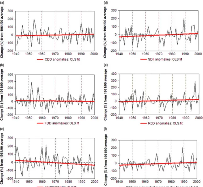
The existence of significant trends in anomaly time series was also investigated using the described method-ology. In each year, the anomalies of the indices time series were calculated from the base period of 1961–1990 by standardizing the individual station’s series using the climatological average and standard deviation of the base period. The regional-average anomaly series were com-puted using the full set of 19 stations’ series (Figure 4) and the analysis period was set to 1940–2000. As all stations do not contain complete data in this period, the regional anomaly of a year was obtained by weighting the anomalies according to the number of stations available for that year (Frich et al., 2002).
Any cyclical components in the variation of time series make it difficult to see the underlying trend. Aiming to improve our understanding of the indices time series, smoothing techniques were used to reduce random fluctuations and provide a clearer view of their underlying behaviour. Moving windows with a time span of 5 and 10 years were used to compute moving average series of the extreme precipitation indices. For the sake of simplicity, these series are denominated the temporal average of extremes (TAE) series. Moving 5 and 10 years, standard deviation statistics of the indices were also computed in order to analyse the temporal evolution
of their variability. These series are denominated the temporal variability of extremes (TVE) series. The TAE and TVE series were calculated for each station and were then averaged over the 15 stations to obtain the regional-average TAE and TVE series for the period 1955/1999. 3.4. Results and discussion
A regional correlation analysis, averaging the Spearman rank-order correlation coefficients of the six indices over the 15 stations, revealed that the dryness indices (CDD, FDD, AII) might provide information that is essentially different from the three wetness indices (SDII, R5D, R30), because they are uncorrelated with any of them. Nevertheless, the correlations between AII and the three wetness indices have positive signs, whereas the other two dryness indices show negative signs when correlated with the wetness indices. Interestingly, the correlation between AII and SDII is extremely weak. The correlation between CDD and FDD is negative but weak, which might indicate that an increase (decrease) in the length of the greatest dry spell will not necessarily entail a significant decrease (increase) in the mean frequency of dry events. The three wetness indices are moderately positively correlated with each other.
The results of the Shapiro–Wilk test indicate that most series of the R5D and R30 indices (87% and 93% of the stations, respectively), and 33% of the SDII series, cannot be considered as Gaussian in the period 1955/1999, at the 5% significance level. On the other hand, the normality hypothesis was not rejected for most series of the dryness indices (80% of the CDD series, and 93% of the FDD and AII series).
3.4.1. Trends in extreme indices
Trend estimation results are presented at the 5% and 10% significance levels (Tables V and VI). According to the correlation analysis results, the CDD and FDD indices have oppositely signed trends for most of the stations, although not statistically significant. Hence, these indices do not reflect significant changes neither in the length of dry spells, nor the frequency of dry events. On the other hand, the AII index reflects increases in the magnitude of dryness. A negative station trend in the AII index dominates in the 1955/1999 period, which implies a significant increase of aridity over most of the study region.
The SDII monitors precipitation intensity on wet days and presents significant increasing trends in several stations, but without spatial consistency. A few of them also have significant increasing trends in the maximum 5-day precipitation totals (R5D), but this tendency is not significant for the majority of stations in the R30 index which characterizes the frequency of extremely heavy precipitation events. Accordingly, the extreme indices characterizing wet conditions do not show a clear pattern of significant trends, but rather exhibit different trend signals at the local scale.
These results agree, in general, with those of other studies on regional changes of precipitation for Iberia and Europe (e.g. Klein Tank and K¨onnen, 2003; Haylock and Goodess, 2004; Rodrigo and Trigo, 2007), even though the adopted indices and study period do not always coin-cide and the network of Portuguese stations used in previ-ous studies is coarser. The results from Kostopoulou and Jones (2005), for the period 1958/2000, show regional contrasts over the Eastern Mediterranean in precipitation indices, and significant positive trends were revealed for CDD in many southern stations. Klein Tank and K¨onnen (2003) found no significant trends (5% level) in the annual precipitation indices calculated for the southern region of Portugal within the 1946/1999 period. Simi-larly, the annual indices of precipitation extremes avail-able at the ECA&D project website (http://eca.knmi.nl, retrieved 17 March 2008) do not reveal significant trends within the 1946/2006 period, but the scarce number of stations available in southern European regions, espe-cially in Portugal, makes it difficult to assess local con-trasts. Nevertheless, the seasonal analysis reveals a few significant (5% level) contrasting trends in the South of Portugal within the 1946/2006 period (http://eca.knmi.nl, retrieved 17 March 2008). For example, the frequency of very wet days (R95p) has negative trends at Beja and Tavira in spring; the frequency of extremely wet days (R99p) has a negative trend in Tavira in spring, whereas it has a positive trend in summer (June–August) at Beja. Haylock and Goodess (2004) analysed trends in several extreme precipitation indices over Europe for the winter months (December–February) of the period 1958/2000. In the northwest of the Iberian Peninsula, the results showed a small decrease in CDD, while the rest of the peninsula has seen large increases in this index, except in southern Portugal where the CDD trend magnitudes are small. In contrast, the frequency of very heavy precipi-tation days (R90p index) showed a decrease over most of the peninsula (including the northwest), but a slight increase in the southeast and southern Portugal. Rodrigo and Trigo (2007) investigated annual and seasonal trends in five precipitation variables using data from 22 stations scattered across the Iberian Peninsula, aiming to analyse the behaviour of daily rainfall in the period 1951–2002. Among those stations, five of them are located in southern Portugal (Lisboa, Grˆandola, Serpa, Rel´ıquias and Mon-forte). Only a few significant trends (5% level) were found for these five stations, most of them at Rel´ıquias, and the variables characterizing extreme events do not show a clear pattern at the local scale. For example, Rodrigo and Trigo (2007) showed that the 95th per-centile and the percentage of rain falling on days with rainfall above the 95th percentile have negative trends at Rel´ıquias in all seasons and for yearly values, but Serpa has increasing trends for yearly values. Moreover, these variables have significant decreasing trends at Grˆandola in spring and summer.
The trend results of the anomaly time series (Table VI) are exactly the same as the precipitation indices results (Table V) as far as the trend signals are concerned, but
T able V . T rends in precipitation indices estim ated with the OLS m odel (O), the Autor egr essive err o r m odel (A) and with the Heter o scedastic linear m odel (H), for the period 1955/99. Significance of trends assessed u sing the M ann – K endall test: v alues in bold face are significant at < 5% level (m arked with ∗∗)a n d < 10% level (marked with ∗). Station C ode CDD F DD AII S DII R 5D R30 Comporta 23E.01 − 0.0094 (O) 0 .0066 (O) − 0 .0007 (O) 0 .0394 ∗∗ (A) 0 .8518 ∗∗ (O) 0 .0566 ∗ (H) S ˜ao Man ¸cos 23K.01 0 .0558 (A) − 0.0086 (O) − 0 .0029 ∗∗ (O) 0 .0156 (O) 0 .5813 ∗ (A) 0 .0040 (O) Azinheira B arros 25G.01 − 0.1734 (O) 0 .0154 (O) − 0 .0011 (O) 0 .0066 (H) 0.1577 (O) 0 .0194 (O) Ferreira d o A lentejo 25I.01 0 .1489 (O) − 0.0067 (O) − 0 .0032 ∗ (H) 0 .0250 ∗∗ (A) 0 .3814 ∗ (H) − 0 .0130 (O) Pedrog ˜ao do Alentejo 25L.01 0 .2258 (O) − 0.0061 (O) − 0 .0039 ∗∗ (A) − 0.0117 (A) 0 .1358 (H) − 0 .0093 (A) Santo A leixo d a R estaura ¸c ˜ao 25O.01 − 0.0232 (O) 0 .0202 (O) − 0 .0040 ∗∗ (O) − 0.0106 (H) 0 .0076 (H) − 0 .0144 (A) Aljustrel 26I.03 0 .5369 ∗∗ (H) − 0.0121 (O) − 0 .0032 ∗∗ (H) − 0.0252 (A) − 0.4006 (O) − 0 .0066 (A) Castro V erde 27I.01 − 0.2645 (H) 0 .0497 ∗∗ (A) − 0 .0026 (O) 0 .0056 (O) 0 .1728 (H) − 0 .0030 (O) Aldeia de Palheiros 28H.01 − 0 .0944 ∗∗ (O) 0 .0130 (O) − 0 .0034 ∗∗ (O) 0 .0022 ∗∗ (H) 0 .1886 (O) − 0 .0099 ∗∗ (H) Santana d a S erra 28H.03 0 .6785 ∗∗ (O) − 0.0228 (O) − 0 .0039 ∗ (O) 0 .0636 ∗∗ (H) 0 .7582 ∗ (H) 0 .0304 (H) Barragem d a B ravura 30E.03 − 0.1025 (H) − 0.0048 (A) − 0 .0021 (O) 0 .0306 ∗ (H) 0 .5972 ∗∗ (O) 0 .0617 ∗∗ (H) Sobreira 30I.02 − 0.1640 (O) 0 .0168 (A) − 0 .0034 ∗∗ (O) 0 .0588 ∗∗ (H) 0 .7732 ∗ (A) 0 .0377 (H) Picota 30K.02 − 0.3487 (A) 0 .0141 (H) − 0 .0023 ∗ (O) − 0.0238 (O) − 0.0183 (H) − 0 .0102 (O) Alcaria (Castro M arim) 30L.04 0 .0925 (O) − 0.0194 (O) − 0 .0005 (O) − 0.0124 (O) 0 .6295 (O) − 0 .0014 (O) Lisboa Geof ´ısica 675 − 0.0939 (H) − 0.0080 (O) − 0 .0022 (O) − 0.0038 (O) 0 .1533 (H) 0 .0022 (H) T able V I. T rends in anom aly tim e series o f p recipitation indices estim ated with the OLS m odel (O), the Autor egr essive err o r m odel (A) and with the Heter o scedastic linear m odel (H), for the period 1955/99. Significance of trends assessed u sing th e M ann – K endall test: v alues in bold face are significant at < 5% level (m arked with ∗∗ )a n d < 10% level (marked with ∗). Station C ode CDD F DD AII S DII R 5D R30 Comporta 23E.01 − 0.0003 (O) 0 .0034 (O) − 0 .0064 (O) 0 .0267 ∗∗ (A) 0 .0263 ∗∗ (O) 0 .0301 ∗ (H) S ˜ao Man ¸cos 23K.01 0 .0021 (A) − 0.0049 (O) − 0 .0213 ∗∗ (O) 0 .0116 (O) 0 .0278 ∗ (A) 0 .0026 (O) Azinheira B arros 25G.01 − 0.0083 (O) 0 .0078 (O) − 0 .0081 (O) 0 .0067 (H) 0.0072 (O) 0 .0113 (O) Ferreira d o A lentejo 25I.01 0 .0067 (O) − 0.0033 (O) − 0 .0234 ∗ (H) 0 .0208 ∗∗ (A) 0 .0243 ∗ (H) − 0 .0113 (O) Pedrog ˜ao do Alentejo 25L.01 0 .0083 (O) − 0.0031 (O) − 0 .0283 ∗∗ (A) − 0.0053 (A) 0 .0057 (H) − 0 .0045 (A) Santo A leixo d a R estaura ¸c˜ao 25O.01 − 0.0009 (O) 0 .0095 (O) − 0 .0299 ∗∗ (O) − 0.0086 (H) 0 .0003 (H) − 0 .0081 (A) Aljustrel 26I.03 0 .0235 ∗∗ (H) − 0.0044 (O) − 0 .0250 ∗∗ (H) − 0.0117 (A) − 0.0196 (O) − 0 .0041 ∗∗ (A) Castro V erde 27I.01 − 0.0126 (H) 0 .0273 ∗∗ (A) − 0 .0181 (O) 0 .0045 (O) 0 .0090 (H) − 0 .0016 ∗∗ (O) Aldeia de Palheiros 28H.01 − 0.0038 (O) 0 .0060 (O) − 0 .0234 ∗∗ (O) 0 .0018 (H) 0 .0083 (O) − 0 .0051 ∗∗ (H) Santana d a S erra 28H.03 0 .0259 ∗∗ (O) − 0.0123 (O) − 0 .0244 ∗ (O) 0 .0377 ∗∗ (H) 0 .0254 ∗ (H) 0 .0136 (H) Barragem d a B ravura 30E.03 − 0.0037 (H) − 0.0024 (A) − 0 .0175 ∗ (O) 0 .0144 (H) 0 .0198 (O) 0 .0182 (H) Sobreira 30I.02 − 0.0059 (O) 0 .0075 ∗ (A) − 0 .0225 ∗∗ (O) 0 .0254 ∗∗ (H) 0 .0224 ∗ (A) 0 .0104 (H) Picota 30K.02 − 0 .0164 ∗ (A) 0 .0103 (H) − 0 .0198 ∗∗ (O) − 0 .0085 ∗ (O) − 0.0005 (H) − 0 .0030 (O) Alcaria (Castro M arim) 30L.04 0 .0034 (O) − 0.0098 (O) − 0 .0039 (O) − 0.0041 (O) 0 .0140 (O) − 0 .0006 (O) Lisboa Geof ´ıs ica 675 − 0.0010 (H) − 0.0035 (O) − 0 .0166 (O) − 0.0027 (O) 0 .0055 (H) 0 .0009 ∗ (H)
Figure 5. Differences in the average extreme indices’ values between 1940 and 2000 from the average 1961/90 value of weighted regional stations. The trend of the AII annual anomalies series (c) is significant at the 6% level. This figure is available in colour online at
www.interscience.wiley.com/ijoc the trends significance is different for a few stations and
indices. Coherent spatial patterns of statistically signifi-cant changes emerge in the magnitude of dryness (AII), while the remaining anomaly time series show a lack of spatial consistency. The remaining indicators show mixed patterns of change but significant increases have occurred in the extreme amount derived from short-term precipita-tion intensity (R5D) in five staprecipita-tions, while for other three stations significant decreases in the number of heavy rain-fall events (R30) have occurred. The existence of signif-icant trends in the regional-average anomaly time series was also investigated (Figure 5) using 19 stations’ data for the period 1940–2000. As discussed before, absence of spatial consistency and/or significant trends character-izes the majority of the precipitation indices calculated, except for the AII index. Therefore, not surprisingly, this was the only index with a significant decreasing trend (the p-value of the Mann–Kendall test is equal to 0.06) in the regional-average anomaly time series (Figure 5(c)), indicating an increase of dryness over the study region.
The low spatial coherence of the trends found in the anomaly time series is consistent with the mixed pattern of positive and negative changes shown in the maps of the globe and it is especially noticeable in southern European regions (Frich et al., 2002). For example, the SDII has increased over many parts of Europe, southern Africa, USA and parts of Australia, although the patterns of change are also variable in these parts of the world showing some relatively nearby stations with opposite signs of change (Frich et al., 2002). Absence of spatial consistency also characterizes the majority of the anomaly time series of the precipitation indices for the Eastern Mediterranean (Kostopoulou and Jones, 2005).
3.4.2. Dynamic temporal evolution of extremes
Moving window statistics (mean and standard deviation) with a time span of 5 and 10 years were computed for each station, and then averaged over the 15 stations to obtain a regional-average. This is a very useful approach because non-linear trends in precipitation extremes can
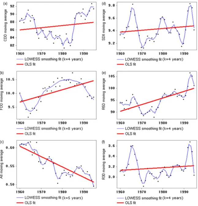
Figure 6. Ordinary least squares fitting (OLS, thick line) and weighted local polynomial fitting (LOWESS smoothing, thin line) for each regional-average TAE series (moving average of the extreme index using a time span of 10 years), for the period 1955/99. This figure is
available in colour online at www.interscience.wiley.com/ijoc be revealed, and periods with distinct climatic variability
can be identified. The results obtained using windows with a time span of 5 years are identical to the ones obtained with a time span of 10 years, but a little noisier. For this reason, and for the sake of simplicity, only the latter are presented. The moving average series of the extreme precipitation indices was named TAE series. The temporal dynamics underlying these series were captured through weighted local polynomial models (LOWESS smoother proposed by Cleveland, 1979) fitted with a time span of k years determined by generalized cross-validation. In order to point out any non-linear trends underlying the TAE series, simple linear regression models, estimated by OLS, were also fitted.
For all of the precipitation indices considered, the results show non-linear trends in the TAE series within the 1955/1999 period at the large majority of stations.
These results might explain why the regression models fitted to the indices time series could not significantly capture the trend signal for the majority of the stations’ indices. Figure 6 shows the results of the regional-average TAE series of the six indices. The non-linear trends and cyclic patterns of the individual stations’ TAE series (not shown) are identical to the ones illustrated in Figure 6 (any exceptions are referred in the text), but much more sharpen.
As expected from the previous results, the TAE series of AII clearly reflect a strong increase in the magnitude of dryness during the period 1955/1999. The maximum length of dry spells, characterized by the TAE series of CDD, has a decreasing trend until the middle of the 1980s and then suddenly increases, keeping a positive trend through the last decade of the twentieth century. One exception occurs at Pedrog˜ao do Alentejo (25L.01) where