URBAN LAND USE CHANGE ANALYSIS AND
MODELING: A CASE STUDY OF SETÚBAL AND
SESIMBRA, PORTUGAL
Master Thesis
By
Yikalo Hayelom Araya
Institute for Geoinformatics
University of
MünsterMünster March 2, 2009
URBAN LAND USE CHANGE ANALYSIS AND
MODELING: A CASE STUDY OF SETÚBAL AND
SESIMBRA, PORTUGAL
. By
Yikalo Hayelom Araya
Supervisor:
Prof. Dr. Edzer Pebesma (University of Münster, Germany)
Co-supervisors:
Prof. Dr. Pedro Cabral (New University of Lisbon, Portugal)
Prof. Dr. Mario Caetano (New University of Lisbon, Portugal)
Prof. Dr. Michael Gould (University Jaume I Castellon, Spain)
Declaration of originality
This is to certify that the work is entirely my own and not of any other person, unless explicitly acknowledged (including citation of published and unpublished sources). The work has not previously been submitted in any form to the University of Münster or to any other institution for assessment for any other purpose.
Signed ___ __________________________________
Abstract
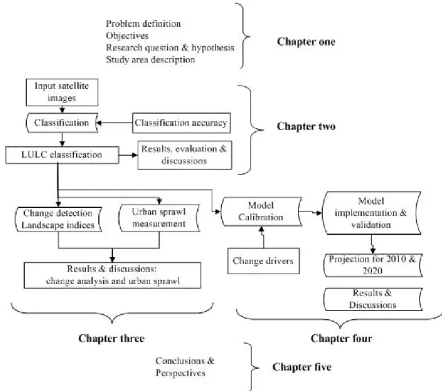
In this paper urban land use change analysis and modeling of the Concelhos of Setúbal and Sesimbra, Portugal is accomplished using multitemporal and multispectral satellite images acquired in the years 2000 and 2006 and other vector datasets. The LULC maps are first obtained using an object-oriented image classification approach with the Nearest Neighbour algorithm in Definiens. Classification is assessed using the overall accuracy and Kappa measure of agreement. These measures of accuracies are above minimum standard accepted levels. The land use dynamics, both for pattern and quantities are also studied using a post classification change detection technique together with the following selected spatial/landscape metrics: class area, number of patches, edge density, largest patch index, Euclidian mean nearest neighbor distance, area weighted mean patch fractal dimension and contagion. Urban sprawl has also been measured using Shannon Entropy approach to describe the dispersion of land development or sprawl. Results indicated that the study area has undergone a tremendous change in urban growth and pattern during the study period. A Cellular Automata Markov (CA_Markov) modeling approach has also been applied to predict urban land use change between 1990 and 2010 with two scenarios: MMU 1ha and MMU 25ha. The suitability maps (change drivers) are calibrated with the LULC maps of 1990 and 2000 using MCE and a contiguity filter. The maps of 1990 and 2000 are also used for the transition probability matrix. Then, the land use maps of 2006 are simulated to compare the result of the “prediction” with the actual land use map in that year so that further prediction can be carried out for the year 2010. This is evaluated based on the Kappa measure of agreement (Kno, Klocation and Kquanity) and produced a satisfactory level of accuracy. After calibrating the model and assessing its validity, a “real” prediction for the year 2010 is carried out. Analysis of the prediction revealed that the rate of urban growth tends to continue and would threaten large areas that are currently reserved for forest cover, farming lands and natural parks. Finally, the modeling output provides a building block for successive urban planning, for exploring how and when urban growth is occurring, and for helping subsequent research works.
Acknowledgments
To the most High God be glory great things He has done. I acknowledge Your great provisions, protections and support throughout the duration of this course and my life.
I remain indebted to my supervisors Prof. Dr. Edzer Pebesma, Prof. Dr. Pedro Cabral, Prof. Dr. Mario Caetano and Prof. Dr. Michael Gould for the discussions and guidelines provided.
I would like to express my deepest gratitude to the Portuguese Geographic Institute, Remote Sensing Unit in general and Prof. Dr. Mario Caetano and Antonio Nunes in particular for providing me all the data required for the study and arranging all the infrastructures to collect the data. I would also like to express my heartfelt gratitude to Prof. Dr. Marco Painho, Prof. Dr. Pedro Cabral and Dr. Filomena Caria for arranging the facilities during my stay in Lisbon for data collection. I am also grateful to Paulo Morgado and Sofia Morgado at the University of Alameda for providing me information related to the legislation. I thank also my friend Nick for helping me during my stay in Lisbon.
I remained indebted to Prof. Thomas Kohler, Prof. Steve Drury, Robert Burstcher, Dr. Christoph Brox, Mohamed Bishr and Prof. Dr. Werner Kuhn for their moral support through out the duration of the program. I am also grateful to all Erasmus Mundus 2007 intake classmates.
I am also grateful to my friends Francis Mwambo and Benedict Mugambi for supporting me during collecting samples for accuracy assessment.
Last but not least I would like to express my heartfelt gratitude to my beloved parents, brothers and sisters who encouraged me morally in my school life.
Table of Contents
Abstract ... iv Acknowledgements ... v List of tables... ix List of figures ... x Acronyms ... xi CHAPTER 1 ... 1 INTRODUCTION ... 1 1.1: Study background ... 1 1.2: Statement of problem ... 2 1.3: Study area... 21.3.1: The Concelhos of Setúbal and Sesimbra ... 3
1.3.2: The Natural Park of Setúbal and Sesimbra ... 3
1.4: Aim and objectives... 4
1.5: Research hypothesis and questions ... 5
1.6: Dissertation structure ... 5
1.7 Tools used in the study ... 6
1. 8 Significance of the study ………...6
CHAPTER 2 ... 7
REMOTE SENSING IMAGE ANALYSIS AND CLASSIFICATION ... 7
2.1: Introduction... 7
2.2: Remote sensing for urban studies ... 8
2.3 Spatial data and processing ... 8
2.3.1: Baseline and charactestics of data used ... 9
2.3.2: Pre-processing and Minimum Mapping Unit (MMU)... 10
2.4: Image classification paradigm for image analysis ... 11
2.4.1: Pixel-based paradigm ………...………12
2.4.2: Object-based paradigm……….………12
2.4.3: Advanced classification approaches……….………12
2.5.1: Multi-resolution segmentation ... 13
2.5.2: Image classification algorithms ... 14
2.5.3: Image classification validation... 15
2.6: Results and evaluation of classification ... 15
2.6.1: Land use classification ... 15
2.6.2: Evaluation of classification results using descriptive analysis ... 18
2.7: Discussions... 21
CHAPTER 3 ... 212
URBAN LAND USE CHANGE DETECTION AND ANALYSIS ... 22
3.1: Introduction... 22
3.2: Urban land use change detection ... 23
3.2.1: Change detection: conceptual framework... 22
3.2.2: Application and approaches of detection techniques... 23
3.3: Post-classification detection technique used... 24
3.4: Results of change detection in Setúbal and Sesimbra... 24
3.5: Urban land use change analysis ... 25
3.6: Quantification and description of urban land use in Setúbal and Sesimbra.... 26
3.6.1: Class Area (CA) ... 26
3.6.2: Number of patches ... 27
3.6.3: Edge Density (ED) ... 27
3.6.4: Largest Patch Index (LPI) ... 27
3.6.5: Area Weighted Mean Patch Fractal Dimension (FRAC_AM) ... 27
3.6.6: Euclidean Mean Nearest Neighbour (ENN_MN)... 28
3.6.7: Contagion ... 28
3.7: Analysis of landscape indices in the Concelhos of Setúbal and Sesimbra .... 28
3.8: Urban sprawl measurement using Shannon entropy... 30
3.8.1: Urban sprawl: built up areas as indicator of urban sprawl... 30
3.8.2: Measurement of urban sprawl in Setúbal and Sesimbra ... 31
3.9: Urban sprawl in Setúbal and Sesimbra ... 33
3.9.1: The on-going sprawl in Setúbal and Sesimbra... 33
3.9.2: Population density and urban sprawl ... 34
CHAPTER 4 ... 37
URBAN LAND USE CHANGE MODELING ... 37
4.1: Introduction... 37
4.2: Land use change models ... 37
4.2.1: Urban land use models... 37
4.2.2: Cellular Automata ... 38
4.3: Modellig in Idrisi ... 40
4.4: Modeling urban land use in Setúbal and Sesimbra ... 41
4.4.1: Introduction... 41
4.4.2: Model description ... 42
4.5: Model Calibration ... 42
4.5.1: Original data and criteria development... 43
4.5.2: MCE: the Boolean approach ... 44
4.5.3: MCE: standardization and weighting of factors ... 45
4.6: Model implementation and validation ... 49
4.6.1: Model implementation ... 49
4.6.2: Model validation ... 50
4.7: Urban land use prediction for the year 2010... 51
4.8: Discussions... 53
CHAPTER 5 ... 54
CONCLUSIONS AND PERSPECTIVES... 54
5.1: Conclusions... 54
5.2: Perspectives and future works... 55
List of tables
Table 2.1 Characteristics of the satellite data used ... 9
Table 2.2 Land cover classes ... 11
Table 2.3 Error matrix: image classification of 2006 (MMU 25ha) ... 20
Table 2.4 Error matrix: image classification of 2000 (MMU 1ha) ... 20
Table 2.5 Error matrix: image classification of 2006 (MMU 1ha) ... 20
Table 3.1 Spatial metrics adopted and used ... 26
Table 3.2 Landscape indices and percentage of changes ... 29
Table 3.3 Shannon’s Entropy values of Setúbal and Sesimbra... 33
Table 3.4 Differences of Shannon Entropy... 34
Table 3.5 Population size and built-up areas (Freguesia-based)... 35
Table 4.1 Existing urban land use models ... 39
Table 4.2 Transitional probablity matrix ... 42
Table 4.3 Boolean approach criteria development... 45
Table 4.4 Fuzz Module: standardization of variables ... 46
Table 4.5 Weights assigned to the variables ... 48
Table 4.6 Results of the validation analysis... 51
Table 4.7 Urban class area of the reference and simulated maps ... 51
List of figures
Figure 1.1 The AML with the Concelhos of Setúbal and Sesimbra ... 3
Figure 1.2 The natural parks “protected areas”of Setúbal and Sesimbra... 4
Figure 1.3 Dissertation structure ... 5
Figure 2.1 Methodology employed to classify images and validate their accruacy ... 7
Figure 2.2 The Four spectal bands (palette gray) and RGG of LISS-III... 10
Figure 2.3 Image classification methods... 12
Figure 2.4 Segmented image... 14
Figure 2.5 LULC maps of 1990, 2000 and 2006 ... 16
Figure 2.6 Simplifed LULC maps of 1990, 2000 and 2006... 17
Figure 3.1 Methodology employed to detect and analyze changes ... 22
Figure 3.2 Urban land use change maps ... 25
Figure 3.3 Temporal urban grwoth signatures of spatial metrics... 29
Figure 3.4 Buffer zones around the city of Sesimbra... 32
Figure 3.5 Buffer zones around the city of Setúbal ... 32
Figure 3.6 The 11 “Freguesia” of Setúbal and Sesimbra ... 33
Figure 3.7 Three Year’s entropy values... 34
Figure 3.8 Differences in entropy values in each pair of years... 34
Figure 3.9 Population density in each “Freguesia”... 35
Figure 4.1 Neighborhood relationship ... 40
Figure 4.2 Components of Cellular Automta (CA)... 40
Figure 4.3 Model Calibration and validation methods... 42
Figure 4.4 Map variables derived after standdardization... 47
Figure 4.5 The rating assigned to each of the factors considered ... 48
Figure 4.6 Suitablity map... 49
Figure 4.7 Actual and predicted land use maps of 2006 ... 50
Acronyms
AML: Greater Metropolitana de Lisboa “Lisbon Metropolitan Area” CA: Cellular Automata
CA_Markov: Cellular Automata Markov Chain Analysis CA/TA: Class/total area
DEM: Digital Elevation Models
DGRUPD: Directorate General of Regional Planning and Urban Development ED: Edge Density
EEA: European Environmental Agency EIA: Environmental Impact Assessments
ENN_MN: Euclidean Mean Nearest Neighbour Distance FRAC_AM: Area Weighted Mean Patch Fractal Dimension GIS: Geographic Information Systems
IPG: Portuguese Geographic Institute IRS: Indian Remote Sensing
LIP: Largest Patch Index LULC: Land Use/Land cover MCE: Multi-Criteria-Evaluation MIR: Mid Infrared
MMU: Minimum Mapping Unit
NRSA: National Remote Sensing Agency NIR: Near Infrared
NP: Number of Patches RS: Remote Sensing SWIR: Short Wave Infrared TIR: Thermal Infrared
CHAPTER 1
INTRODUCTION
1.1: Study background
The history of urban growth indicates that urban areas are the most dynamic places on the Earth’s surface. Despite their regional economic importance, urban growth has a considerable impact on the surrounding ecosystem (Yuan et al., 2005). Most often the trend of urban growth is towards the urban-rural-fringe where there are less built-up areas, irrigation and other water management systems. In the last few decades, a tremendous urban growth has occurred in the world, and demographic growth is one of the major factors responsible for the changes. By 1900 only 14% of the world’s population was residing in urban areas and this figure had increased to 47% by 2000 (Brockerhoff, 2000). The report also revealed that by 2030, the percentage of urban population is expected to be 60%. Urban growth is a common phenomenon in almost all countries over the world though the rate of growth varies. Currently, these are the major environmental concerns that have to be analyzed and monitored carefully for effective land use management. The rapid urban growth and the associated urban land cover changes have also attracted many researchers.
A substantial amount of data from the Earth’s surface is collected using Remote Sensing (RS) and Geographic Information Systems (GIS) tools. RS provides an excellent source of data from which updated land use/land cover (LULC) information and changes can be extracted, analyzed and simulated efficiently. RS in the form of aerial photography provides comprehensive information of urban changes (Bauer et al., 2003). It is not, however, without limitations: costs of the acquisition and the analogue data format are the most obvious problems. The cost of acquiring data causes many analysts to remain sceptical about the potential of remotely sensed data (Rowlands and Lucas, 2004). It should also be noted that LULC mapping using remote sensing has long been a research focus of various investigators (Civco et al., 2002).
Recent advancement in GIS and remote sensing tools and methods also enable researchers to model and predict urban growth more efficiently than the traditional approaches. Several modeling approaches have also been developed to model and forecast the dynamic urban features. One of the approaches is the Cellular Automata-CA. CA is a dynamical discrete system in space and time that operates on a uniform grid-based space by certain local rules (Alkheder and Shan, 2005, Hand 2005). The CA is consisting of cells and transition rules are applied to determine the state of a particular cell. Its ability to represent complex systems with spatio-temporal behaviour from a small set of simple rules and states made it very interesting for urban studies (Alkehder and Shan, 2005). In this study an integrated approach of GIS, RS and modeling has been applied to identify and analyze the patterns of urban changes and provide quantitative and spatial information on developments of urban areas.
1.2: Statement of the problem
On a global basis, nearly 6.8 million km2 of forest, woodlands and grasslands have been converted to other land uses in the last three centuries (Agarwal et al. 2002) and most of the changes were into urban land use. These changes in land use have significant implications on the Earth’s resources and climate.
On a local basis, the expansion of the city of Lisbon to its highly rural outskirts, overtaking the wide, highly productive basalt plains as well as alluvial areas mostly used for horticultural products, has entailed a systematic abandonment of transitional agricultural practices (Carlos 2002). The land use change analysis carried out by the IGP between 1990 and 2000 also verified these facts. This would have significant impact on the surrounding ecosystem: loss of farming land, forest cover, water depletion, and on the benefits generated from the land. Being located in the coastal areas of the country, the study site attracted various human induced activities, which in return resulted in a loss of land resources. As part of the land use management of the Greater Metropolitana de Lisboa (Lisbon Metropolitan Area or AML), attempts are still made and some green spaces are currently being planned. The Portuguese government has also created several protected areas aiming to reduce and control building speculation, and to protect the natural heritage (Carlos 2002). It has to be noted that some kind of urbanization is still continuing in the protected areas of the region. This reveals that the rate of urban growth is still high in the region. Thus, consideration and careful assessment are required for monitoring and planning land management, urban development and decision making.
1.3: Study area
The study was carried out in two administrative areas in Portugal: Setúbal and Sesimbra. Both administrative areas belong to the AML (Figure 1.1). The AML is a
public collective person of associative nature, and of territorial scope that aims to reach common public interests of the 18 Concelhos “Counties”: Alcochete, Almada, Amadora, Barreiro, Cascais, Lisbon, Loures, Mafra, Moita, Montijo, Oeiras, Palmela, Sesimbra, Setúbal, Seixal, Sintra and Vila Franca de Xira (AML 2005). The
AML has the largest population concentration in Portugal and a dramatic population growth has occurred since the year 1960 (Cabral 2006). This situation became serious with the great urban sprawl that took place from 1940 to 1960 as a result of a general migration from rural areas (Carlos 2002). The urbanization increased tremendously when Portuguese inhabitants of the overseas ex-colonies returned during the 1970’s (Cabral 2006). Based on the Portuguese census data of 2001, the population of the AML is around 2.6 Million-approximately ¼ of the entire Portuguese population. The total area of the AML is also about 2,957.4km2 (AML 2005).
Figure 1.1: The AML with the Concelhos of Setúbal and Sesimbra 1.3.1 The Concelhos of Setúbal and Sesimbra
The study area is located in the southern part of Portugal, specifically in the districts of Setúbal and Sesimbra (Figure 1.1). Setúbal is an urban area, differentiated from a
town, village, or hamlet by size, population density, importance, or legal status1. It is located just beneath the capital Lisbon and on the River Sado. As the capital has grown over the years, it has become wealthier and more urbanized, now essentially being a suburb of Lisbon2. It is located about 40km south of Lisbon with approximately 100,000 inhabitants.
The Concelho Sesimbra is another municipality of Portugal in the district of Setúbal. It lies about 40km south of Lisbon and is situated at the foot of the hills of Arrabida Park (discussed below) with a total area of 195.7km2 and a total 37,567 inhabitants3. Due to its particular position near the mouth of the Sado River and its natural harbour, it attracts the attention of many human activities.
1.3.2 The Natural Park of Setúbal and Sesimbra
The study site is well characterized by the natural reserve “Serra da Arrabida”. The
“Serra da Arrabida” lies between Setúbal and the coast, miles of vast limestone ridges and forests of oaks, bay trees and plant life unique to the peninsula (AML
2005). Arrabiba is a natural park that covers 108km2 area and the Arrabida Hills and Mediterranean-like vegetation and microclimate of the region. The natural reserve
surrounding the river Sado provides all manner of wetland wonders from migratory birds and interesting fish species to unique agricultural and natural landscapes4. 1 http://en.wikipedia.org/wiki/ 2 http://www.enterportugal.com/ 3 http://www.travel-in-portugal.com/ 4 http://www.travel-in-portugal.com/
Moreover, the natural reserve of the Sado Estuary occupies a total area of 23,160 ha, integrated into the Concelhos of Setúbal, Ballina and Palmela. The reserve was created by law due to pollution affecting the estuary of Sado and the danger of damaging the natural heritage of interest existing fauna and flora. It is also a place of nesting for various birds such as storks, flamingos and ducks, and spawning, growth and development of various fish5.
Figure 1.2: The natural parks “protected areas” of Setúbal and Sesimbra
1.4: Aim and objectives
The principal aim of this paper was to apply remotely sensed data, geospatial and modeling tools to detect, quantify, analyze, and forecast urban land use changes. The following were also some of the specific objectives of the paper:
¾ Quantify and investigate the characteristics of urban land use over the study area based on the analysis of satellite images;
¾ Identify whether there have been and will be significant urban land use changes;
¾ Analyze and examine the changes using selected spatial metrics;
¾ Assess the accuracy of the classification techniques using error matrix and Kappa statistics;
¾ Identify and analyze urban sprawl using Shannon entropy approach; ¾ Predict and assess urban future land use changes;
¾ Analyze the specific issues of the urban environment and put forward a recommendation or set of recommendations that may form the basis for a sound solution for sustainable land management.
5
1.5: Research hypothesis and questions
This study is based on the hypothesis that there have been considerable urban land use changes in the study area. It also tests two research assumptions:
1) It is possible to use RS and GIS tools along with modeling techniques to study urban growth analysis and modeling
2) There was a significant urban land use changes and urban sprawl in the study area during the study period
In order to assist the analysis, the following research questions will also be posed: ¾ Have there have been major changes in the urban environment of the study
areas?
¾ What was the spatial extent of the land cover change and where was the highest rate of changes?
¾ What will be the extent of the land use changes in the future? ¾ What were the major deriving forces for the changes?
1.6: Dissertation structure
1.7: Tools used in the study
Various software programs have been used in this study to process, quantify, analyze and model the spatial dataset. For the preliminary data processing, extracting the study area and mosaicing satellite images, ArcGIS 9.2-ArcInfo version was used. An object-oriented image classification was implemented using Definiens 5.0. In order to calculate the metrics, Fragstats was also applied. For the modeling part, CA_Markov chain analysis embedded in Idirisi Kilimanjaro has been used.
1.8: Significance of the study
One of the major impacts of urban land cover dynamics is a shrinking amount of cultivated land through the development of infrastructures and various development projects. Therefore, urban land use change studies are important tools for urban or regional planners and decision makers to consider the impact of urban sprawl. The results of this study would provide information relevant to contribute in the environmental management plans and improve urban planning issues. It is also expected to:
¾ Provide information on the status and dynamics of the urban land use of the area and the use of remote sensing from satellite imagery for such analysis for planners.
¾ Assist environmentalist, regional (urban) planners, and decision makers to consider the potential of geospatial tools for monitoring and planning urban environment
¾ Provide elements for long term bench-mark monitoring and observation relating to resource dynamics
¾ Provide a base line for eventual research follow-up, by identifying specific and important topics that should be considered in greater detail by those interested in the area
CHAPTER 2
REMOTE SENSING IMAGE ANALYSIS AND CLASSIFICATION
2.1: Introduction
The theoretical and practical aspects of urban land use change analysis and modeling applied in this study involve different approaches and datasets. The first step for understanding the dynamic nature of LULC was to generate surface information using remote sensing approaches. In the first place, different datasets such as existing land use maps, satellite data, Digital Elevation Model (DEM), road maps and other vectors maps were acquired from the IGP, remote sensing unit6. Basically, CORINE land cover maps for the years 2000 and 2006 with a Minimum Mapping Unit (MMU) of 25ha and a national land cover map with a MMU of 1ha for the year 1990 were obtained. In addition, the satellite data, for the years 2000 and 2006, used in the study were pre-processed and an object-oriented image classification was employed to generate surface information. The following section presents the overall image processing phases applied to generate LULC information and assess the accuracy of the classification. Figure 2.1 also describes the methodology applied to classify the images, assess and analyze the classification.
Figure 2.1 the methodology employed to classify images and validate their accuracy
6
Remote sensing unit of the IPG is a research and development department integrated in the Geographical Information Research and Management Services Directorate (DSIGIG), which is one of the central operational services of the Portuguese Geographic Institute (IGP). The unit develops its activity in the framework of the mission and functions of IGP, which is a National Agency of the Central Public Administration with the main objective of ensuring the execution of the geographic information policy at a national level.
2.2: Remote sensing for urban studies
GIS and RS are land-related and therefore are very useful in the formulation, implementation and monitoring urban development in the move towards sustainable development strategy detection (Yeh and Li 1997). GIS is a systematic process of
spatial data collection and processing. It can be used to study the environment by observing and assessing the changes and forecasting the future based on the existing situation (Ramachandra and Kumar 2004). RS, on the other hand, is the process of data acquisition through space or air borne sensors without having any contact with the target objects. It allows the acquisition of multispectral, multiresolution and multitemporal data for the land use change analysis and modeling. Both RS and GIS tools have been applied in a number of urban studies to detect, monitor and simulate urban land use changes.
Because of their cost effectiveness and temporal frequency, RS approaches are widely used for change detection analysis (Im et al. 2008). It has also great potential for the acquisition of detailed and accurate surface information for managing and planning urban regions (Herold et al. 2002). However, computer assisted production of spatially detailed and thematically accurate LULC information from satellite image continues to be a challenge for the remote sensing research community (Civco et al. 2002). This is due to the heterogeneous nature of urban environment, which makes discriminating land cover classes difficult. It could also be due to the absence of appropriate classification techniques. However, recent advances in GIS and RS tools and methods have enabled researchers to analyze and detect the dynamic nature of urban features in a more efficient way. Some recent researches have also been directed toward quantitatively describing the spatial structure of urban environments and characterizing patterns of urban structure through the use of remotely sensed data (Herold et al. 2002).
2.3: Spatial data and processing
Satellite data are the bases for various environmental studies and have been used in different application areas (e.g. mapping and detecting of land use changes). However, consideration must be given to the impacts of the sun’s inclination, season of image acquisition and cloud cover. This is because these factors would affect the quantitative analysis of the changes. The impact of the differences of sun’s angle may partially be reduced by selecting data belonging to the same time of the year (Singh 1989). The availability of multitemporal data to produce land cover changes is also useful because it solves the problems associated with single dated land cover information. In this study, multiresolution and multitemporal time series including historical satellite imagery, aerial photographs and other vector datasets were used to determine LULC changes over the study period between 1990 and 2006. In order to analyze the time-series dataset and generate surface information, different approaches were also employed.
2.3.1 Baseline and characteristics of data used
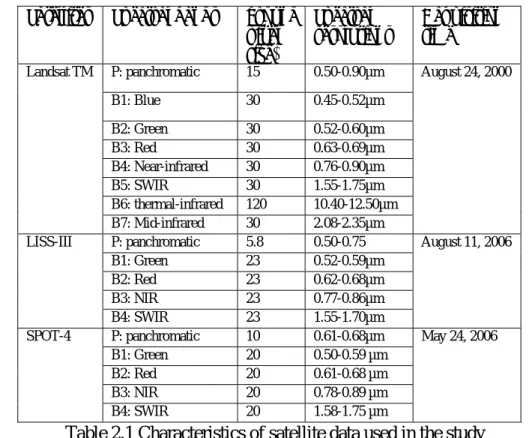
The urban land use change analysis and modeling was based on three LULC maps: 1990, 2000 and 2006 with different MMU, and various ancillary data. In the first place, CORINE7 land cover maps for the years 1990 and 2000 with a MMU of 25ha were acquired from the IGP. A national land cover map with a MMU of 1ha for the year 1990 was also obtained from the IGP. This map was derived from historical Landsat TM images by the remote sensing unit of the IGP8. Moreover, land cover maps with a MMU of 1ha (2000 and 2006) and 25ha (2006) presented at the end of this chapter were derived from the Landsat image of the year 2000, and LISS-III (summer) and SPOT (spring) images of the year 2006. LISS-III is a multi-spectral camera operating in four spectral bands, three in the visible and near infrared (NIR) and one in the short-wave infrared (SWIR) region. The new feature in LISS-III camera is the SWIR band (1.55 to 1.7µm), which provides data with a spatial resolution of 23.5m (NRSA 2003). Similarly, the SPOT-4 is acquired both in the panchromatic and multispectral mode at 10m and 20m resolution, respectively. In the multispectral mode, it acquires images three in the visible and NIR, and one in the SWIR. The spring and summer images were used to better discriminate some land cover classes. The characteristics of the satellite data used in this study are summarized in the Table below.
Satellites Spectral bands ground pixel size) Spectral resolutions Acquisition time P: panchromatic 15 0.50-0.90µm B1: Blue 30 0.45-0.52µm B2: Green 30 0.52-0.60µm B3: Red 30 0.63-0.69µm B4: Near-infrared 30 0.76-0.90µm B5: SWIR 30 1.55-1.75µm B6: thermal-infrared 120 10.40-12.50µm Landsat TM B7: Mid-infrared 30 2.08-2.35µm August 24, 2000 P: panchromatic 5.8 0.50-0.75 B1: Green 23 0.52-0.59µm B2: Red 23 0.62-0.68µm B3: NIR 23 0.77-0.86µm LISS-III B4: SWIR 23 1.55-1.70µm August 11, 2006 P: panchromatic 10 0.61-0.68µm B1: Green 20 0.50-0.59 µm B2: Red 20 0.61-0.68 µm B3: NIR 20 0.78-0.89 µm SPOT-4 B4: SWIR 20 1.58-1.75 µm May 24, 2006
Table 2.1 Characteristics of satellite data used in the study
7
CORINE land cover uses a unique combination of satellite images and other data to reveal all kinds of information on land sources-information which has a broad range of application: from nature conservation to urban planning (EEA, 2000). Computer-assisted image interpretation of earth observation satellite images is used to map the whole European territory into standard CORINE Land cover categories.
8
In order to view and discriminate the surface features clearly, all the input images were composed using the RGB color composition. This is also important for generating a segmented image because the algorithm considers all the input images for segmentation. The four spectral channels that can be generated using the LISS-III and SPOT-4 sensors are similar to bands 2, 3, 4 and 5 of the TM or ETM+ sensors. This reveals that both LISS-III and SPOT-4 are not operating in the blue band. Figure 2.2 shows an example of gray palette of the four spectral bands and RGB composition of the study area in the LISS-III sensor.
Figure 2.2 the four spectral bands (palette gray) and RGB432 of LISS-III
Furthermore, ancillary data such as major road axis maps, existing land cover maps, DEM, high resolution aerial photographs and Google map were integrated in the study. Population data for the census year of 2001 was also used to describe and analyze the pattern of urban sprawl or growth.
2.3.2 Pre-processing and Minimum Mapping Unit (MMU)
¾ Pre-processing:
Satellite data obtained from various sensors undergo some degree of geometric and radiometric distortions due to Earth rotation, platform instability, atmospheric effects, etc. Accurate spatial registration or rectification of the images is thus essential for effective LULC change analysis. This necessitates the use of geometric rectification algorithms that register the images to each other or to a standard map projection (Singh 1989). The input images were corrected and resampled by the Remote Sensing Unit of the IGP. Initially, the satellite data were provided in composite images and as a pre-processing phase, individual bands were extracted in ArcGIS. Consequently, all the bands (4bands-LISS-III, 4bands-SPOT and 6bands-Landsat TM) were obtained for further processing and analysis. The spatial extent covering the entire study area (Setúbal and Sesimbra) was then extracted from the images using spatial analyst tool in ArcGIS. Since a single spring image was not covering the whole study area, two scenes of spring images of the year 2006 were also mosaiced on a band by band basis using Mosaicing tool.
¾ Minimum Mapping Unit (MMU):
MMU is the smallest area that can be mapped. It is selected as close as possible to the original data resolution so as to reduce the loss of specificity introduced in the resampling process. Since only large MMU changes resulted in significant differences
in the accuracy estimates, an analyst may have the flexibility to select from a range of MMU that are appropriate for a given application (Knight and Lunetta 2003). It was
also argued that a possible MMU for a classification created from ETM+ may be 8100m2 or 90*90 m (3*3 pixels) (Knight and Lunetta 2003). As stated, the MMU for the available land cover maps was 1ha (national land cover-1990) and 25ha (CORINE1990 and 2000). The LULC maps were therefore derived with a MMU of 25ha for the year 2006 and 1ha for the year 2000 and 2006.
¾ Land cover nomenclature
The European nomenclature distinguishes 44 different types of land cover classes and each country can supplement the categories with a more detailed level (EEA 2000). The datasets, the land cover maps used in the study, were provided along with the 44 land cover classes. For the sake of simplicity on one hand and because the focus of the study was on urban area on the other hand, the 44 classes were simplified into 7 major classes The land cover classes used and their descriptions are given in Table 2.2. The urban/developed areas exhibit spatially heterogeneous features and discrimination of some of the features still remain a problem. This is because such surface features tend to have similar spectral response. In this case, the “urban class” includes all forms of built structure including commercial, residential, road and other impervious features.
Land cover classes Descriptions based on the CORINE land cover classes
1 Urban or Built up areas This classes both continuous and discontinuous urban fabric, industrial, commercial, transportation and other related built up areas
2 Green urban areas This contains only the Green urban areas 3 Non-irrigated arable
land
It comprises non-irrigated arable land, annual and permanent crops, complex cultivation patterns, agriculture with natural vegetation, etc
4 Irrigated land This mainly contains permanently irrigated land, rice fields, fruit trees and berry plantations
5 Forest cover This is the dominant land cover class in the area and comprises: broad-leaved forest, coniferous forest, mixed forest, transitional woodland/shrub, etc
6 Bare land Sand plains and dunes, bare rock, are considered as bare land 7 Water bodies and marsh
area
Water related features such as water courses, water bodies, estuaries, salt marshes are include in this class
Table 2.2 Land cover classes
2.4 Image classification paradigm for image analysis
RS research focusing on image classification has attracted the attention of many researchers (Lu and Weng 2007) and a number of researches have been conducted using different classification algorithms. It should be noted that valuable surface information extraction and analysis is also well performed using image classification. Image classification is the process of assigning pixels of continuous raster image to predefined land cover classes. It is a complex and time consuming process, and the result of classification is likely to be affected by various factors (e.g. nature of input images, classification methods, algorithm, etc). In order to improve the classification accuracy, thus, selection of appropriate classification method is required. This would
also enable analyst to detect changes successfully. In various empirical studies, different classification methods are discussed and Figure 2.3 summarizes the different types of classification techniques using different criteria for categorization. Two classification paradigms: pixel and object-based as well as advanced classification approaches are discussed below in detail.
Figure 2.3: Image Classification methods 2.4.1 Pixel-based paradigm
In this method, each pixel is classified based on the spatial arrangement of edge features in its local neighbourhood (Im et al. 2008). Image classification at pixel level could be supervised or unsupervised; parametric and hard classifiers. In a supervised classification method (e.g. maximum likelihood), the analyst is responsible for training the algorithm. Input from analyst is very limited in an unsupervised method i.e. specifying number of clusters and labelling the classes. The statistical properties of training datasets from ground reference data are typically used to estimate the probability density functions of the classes (Santos et al. 2006). Each unknown pixel is then assigned to the class with the highest probability at the pixel location. However, a pixel-based method is associated with the mixed-pixel problem and it might not clearly show the required classes of interest, although they are the most commonly used technique. Hence, change detection using this approach may not be effective.
2.4.2 Object-based paradigm
The advent of object-oriented approaches provides a tool for mapping detailed land uses (Mori et al. 2004). This approach considers group of pixels and the geometric properties of image objects. It segments the imageries into homogenous regions based on neighbouring pixels’ spectral and spatial properties. It is based on a supervised maximum likelihood classification. Thus, an object-oriented method has been applied in this project in to avoid the mixed pixel problems. The overall procedure is described below.
2.4.3 Advanced classification approaches
Recently, various advanced image classification approaches have been widely used (Lu and Weng 2007). These include artificial neural networks, fuzzy-set theory,
Image classification approaches Data Distribution Training Algorithm Pixel Class Membership Parametric Non-Parametric Unsupervised Hard Classifiers Soft (Fuzzy) Classifiers Supervised
decision tree classifier, etc. The pixel-based approach is referred to as a “hard” classification approach and each pixel is forced to show membership only to a single class. Soft classification approach is thus developed as an alternative because of its ability to deal with mixed pixels. The soft classification method provides more information and produces potentially a more accurate result (Jensen et al. 2005).
2.5 Image classification and validation techniques used
Analyses of the literature reviewed and analyst’s personal experiences revealed that pixel-based classification produces inconsistent “salt and pepper” output. This is true not only with coarse resolution images but also with fine resolution images (e.g. IKONOS). As stated, recent studies indicated that an alternative object-oriented approach produces better and effective result than the pixel-based does. This is because the world is not pixelated rather it is arranged in objects (Araya and Hergarten 2008). The object-oriented processing technique segments the images into homogenous regions based on neighbouring pixels’ spectral and spatial properties. Image analysis techniques that consider both the measured reflectance values and neighbourhood relations (object-oriented analysis) are available in Definiens and SPRING software packages. Such object-based schemes are essential for urban growth studies (Moeller et al. 2004).
In this study, the Definiens 5.0 software has been used to classify the Landsat, LISS-III and SPOT images. According to the software manufacturer the guiding principle for the land use classification is that objects should be generated as large as possible and as fine as necessary (GmbH 2001)9. The software is based on an object-based processing and classification of remote sensing imagery. It has the capabilities to import images from different data formats, generate object of segments, collect training samples, classify and perform mapping operations. It also supports different methods to train the algorithm and build up resource- and knowledge-based image classification. The image segmentation and object-oriented classification method for change detection holds much promise (Civco et al. 2002). Moreover, object-based analysis offers great potential and opportunities for identifying and characterizing LULC change processes.
2.5.1 Multi-resolution segmentation
The Landsat (bands1-5 and band7), SPOT (four bands) and LISS-III (four bands) images were loaded into Definiens as image layers. One way to include spatial dimensions in image analysis is to identify relatively homogenous regions and treat them as objects using the process of segmentation. Although segmentation is not a new concept, segmentation-based image classification has significantly increased recently (Blaschke 2004). The segmentation process in eCognition is known as a “multi-resolution segmentation” and is based on “region growing approach”. That is a bottom-up region merging approach, where the smallest objects contain single pixels. In the process, smaller objects are merged into larger objects based on the scale parameters defined and spectral properties. The segmentation process stops when the
9
smallest growth of an object exceeds a user defined threshold or scale parameter (Im et al. 2008). The formation of the objects is also carried out in such a way that an overall homogeneous resolution is kept (Mansor et al. 2002). Image segmentation in Definiens 5.0 requires some parameters to be set:
¾ Image layer weights: varying between 0 to 1 indicating the importance of a layer in the segmentation process;
¾ Scale parameter: determines the average size of image objects; ¾ Color: determines the homogeneity of the image;
¾ Shape: controls the degree of object shape homogeneity
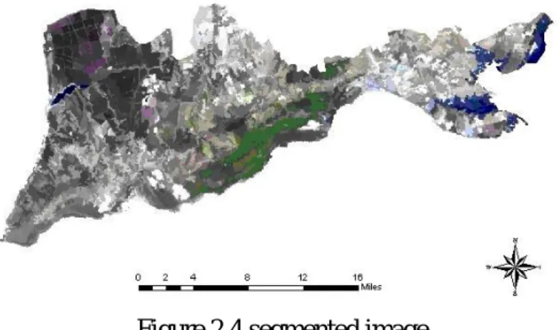
There is no specific agreement or guideline on the rules to be set and these parameters are often set in a trial and error mode as well as visual analysis of the segmented images. In this case, all the image layers were given equal importance 1 and different scale parameters were attempted based on visual analysis of the segmentation results. Figure 2.4 shows one of the segmented images for the Landsat image of 2000.
Figure 2.4 segmented image
For the analysis and classification of image objects, in Definiens 5.0, the land cover classes (Table 2.2) has to be defined in a class hierarchy. Sample objects which are typical representatives of the classes were collected using high resolution images and existing land cover maps.
2.5.2 Image classification algorithm
Land use classification requires a classification scheme and algorithms. As mentioned above, the CORINE land cover classification scheme has been applied to define the land cover classes. The Definiens offers two different classification algorithms: Nearest Neighbour and Membership Functions. The Membership Functions are soft classifiers that are based on a fuzz classification systems, in which the feature values of arbitrary range were translated into a value between 0 (no membership) and 1 (full membership) (Benz et al. 2004). The Nearest neighbour classification is similar to supervised classifications in common image analysis software. The classifier was applied by using the Edit Standard Nearest Neighbour Feature Space Tool. For each class, the standard nearest neighbour expression was inserted. After constructing the resource based sample collection, a standard nearest neighbour algorithm was applied
to produce the land cover map. Based on these procedures, land cover maps of the study area have been produced.
2.5.3 Image classification validation
Accuracy assessment is a process used to estimate the accuracy of image classification by comparing the classified map with a reference map (Caetano et al. 2005). It is critical for a map generated from any remote sensing data. Although accuracy assessment is important for traditional photographic remote sensing techniques, with the advent of more advanced digital satellite remote sensing the necessity and possibility of performing advanced accuracy assessment have received new interest (Congalton 1991). Currently, accuracy assessment is considered as an integral part of any image classification. This is because image classification using different classification algorithms may classify pixels or group of pixels to wrong classes. The most obvious types of error that occurs in image classifications are errors of omission or commission.
The common way to represent classification accuracy is in the form of an error matrix. An error matrix is a square array of rows and columns and presents the relationship between the classes in the classified and reference maps. Using error matrix to represent accuracy is recommended and adopted as the standard reporting convention (Congalton 1991). In this paper, overall, producer’s and user’s accuracy were considered for analysis. The Kappa coefficient, which is one of the most popular measures in addressing the difference between the actual agreement and change agreement, was also calculated. The Kappa statistics is a discrete multivariates technique used in accuracy assessment (Fan et al. 2007).
The reference data used for accuracy assessment are usually obtained from aerial photographs, high resolution images (e.g. IKONOS, QUICKBIRD, and aerial photo), and field observations. In this case, the assessment was carried out using high resolution (50cm) aerial photograph as a reference. A set of reference points has to be generated to assess accuracy and 240 stratified random points were generated for each derived maps. These points were verified and labelled against the reference data. Error matrices were then designed to assess the quality of the classification accuracy of all the maps. The error matrix can be used as a starting point for a series of descriptive and analytical statistical techniques (Congalton 1991). The overall, user’s and producer’s accuracies, as well as the Kappa statistic were then derived from the matrices. By introducing the methodologies employed to classify the images and assess the accuracy in the study, the results are presented in the following section.
2.6 Results and evaluation of classification
2.6.1 Land use classification
In order to facilitate the task of mapping relatively homogeneous areas over different time periods to enable spatio-temporal analysis, geospatial tools are very essential. The presence of multitemporal satellite data also provided an opportunity to generate
land cover maps of the areas with different MMU and observe the changes in urban characteristics. The figures shown below have been derived using an object-oriented image analysis to detect, quantify and simulate the changes.
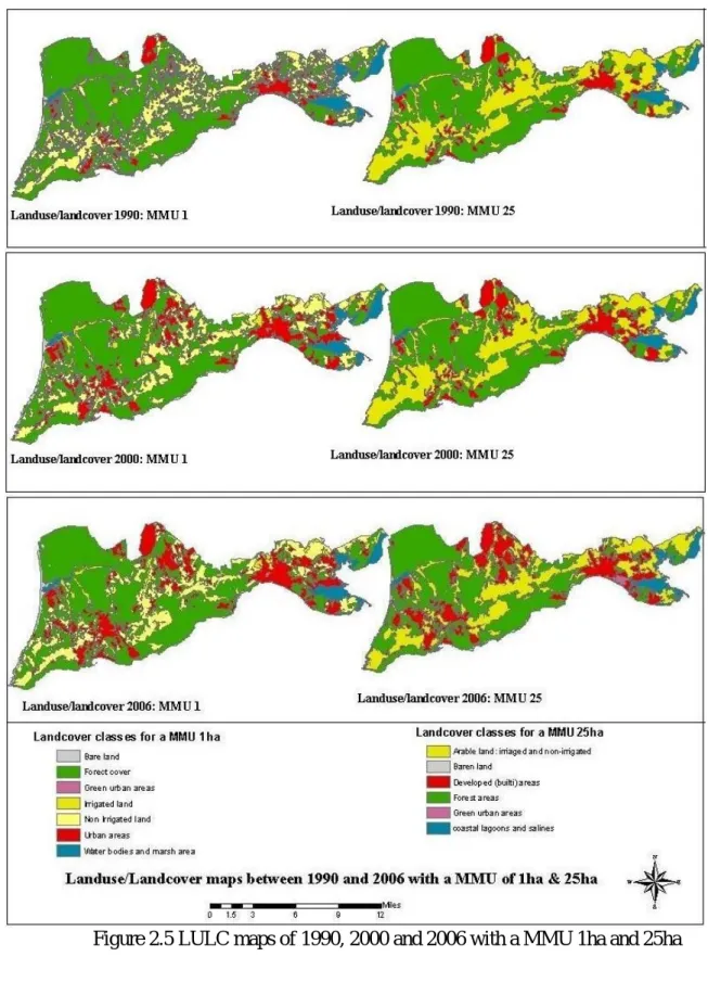
Figure 2.5 LULC maps of 1990, 2000 and 2006 with a MMU 1ha and 25ha
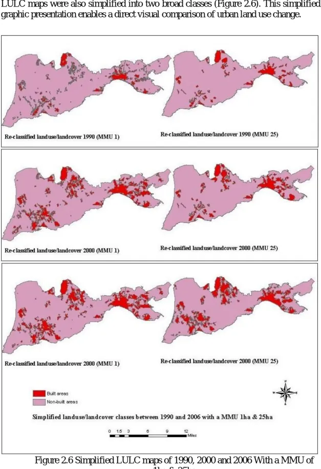
Furthermore, in order to examine the nature and spatial extent of built-up areas, the LULC maps were also simplified into two broad classes (Figure 2.6). This simplified graphic presentation enables a direct visual comparison of urban land use change.
Figure 2.6 Simplified LULC maps of 1990, 2000 and 2006 With a MMU of 1ha & 25ha
2.6.2 Evaluation of classification results using descriptive analysis
In order to use the derived land cover maps for further change analysis, the errors need to be quantified and evaluated in terms of classification accuracy. As stated, an accuracy assessment was carried out and the result of the matrix is presented in Tables 2.3, 2.4 and 2.5. The technique provides some statistical and analytical approaches (in the form of user’s, producer’s and overall accuracies) to examine the accuracy of the classification. The Kappa analysis was also calculated from the error matrix.
¾ Overall accuracy
This is computed by dividing the total correct number of pixels (i.e. summation of the diagonal) to the total number of pixels in the matrix (grand total). The overall accuracies for the maps of 2000 and 2006 with a MMU of 1ha were 92.51% and 87.68%, respectively. Similarly, the overall accuracy of the 2006 map with a MMU of 25ha was 89.17%. Various standard threshold levels were applied to the lower and higher tail of each distribution in order to find the threshold value that produced the highest change classification accuracy (Mas 1999). In some empirical studies (Anderson et al., 1976), it is noted that a minimum accuracy value of 85% is required for effective and reliable land cover change analysis and modeling. Therefore, the classification carried out in this study produces an overall accuracy that fulfils the minimum accuracy threshold defined by Anderson.
¾ Producer’s accuracy
This refers to the probability of a reference pixel being classified correctly. It is also known as omission error because it only gives the proportion of the correctly classified pixels. It is obtained by dividing the number of correctly classified pixels in the category by the total number of pixels of the category in the reference data. The overall result of the producer’s accuracy ranges from 60% to 100%. The lowest producer’s accuracy exists in the land cover classes “arable” and “urban areas”. This is probably attributed to the similar spectral properties of some of the land cover classes (e.g. bare land with urban areas, green urban areas with forest cover, arable during dry season with bare land, etc).
¾ User’s accuracy
This assesses the probability that the pixels in the classified map or image represent that class on the ground (Congalton 1991). It is obtained by dividing the total number of correctly classified pixels in the category by the total number of pixels on the classified image. User’s accuracy of individual classes ranges from 63% to 100%. From user’s accuracy point of view, urban areas and bare land presented low accuracy for the land cover map 2000 (1ha MMU). The “urban class” and bare land were, to some extent, misclassified as “non-irrigated land” and urban areas, respectively. This is probably caused by the spectral signature of the features.
¾ Kappa coefficient
The Kappa coefficient, which is a measure of agreement, can also be used to assess the classification accuracy. It expresses the proportionate reduction in error generated by a classification process compared with the error of a completely random classification (Congalton 1991). The Kappa statistic incorporates the off-diagonal elements of the error matrices (i.e., classification errors) and represents agreement obtained after removing the proportion of agreement that could be expected to occur by chance. The Kappa coefficient is calculated using the information in Tables 2.3, 2.4 and 2.5 and the following formula given by Congalton, 1991.
, 1 ) 1 ( 2 1 1 ) 1 ( ii ∑ = × + − ∑ = − ∑= × + = + + r i X Xi N r i r i X Xi X N K
(Adopted from Congalton 1991) Where:
r = is the number of rows in the matrix
Xii = is the number of observations in rows i and column I (along the major diagonal) Xi+ = the marginal total of row i (right of the matrix)
Xi+1 are the marginal totals of column i (bottom of the matrix) N is the total number of observations.
It is not uncommon that the Kappa coefficient appears to be low, giving the impression that the classification of remote sensing performed better than chance only by K point of proportion (Muzein 2006). It was calculated to be 0.86, 0.86 and 0.83 for the land cover maps of 2006 (MMU 25), 2000 (MMU 1ha) and 2006 (MMU 1ha), respectively. These Kappa results are considered to be a good result.
Table 2.3 Error matrix: image classification of 2006 (MMU 25ha)
Table 2.4 Error matrix: image classification of 2000 (MMU 1ha)
Reference map
Urban areas Green urban Arable Forest cover Bare land Water bodies & marsh areas Grand Total User’s accuracy
Urban areas 140 4 12 4 160 88.00 Green urban 24 210 6 240 88.00 Arable 2 34 4 40 85.00 Forest cover 10 190 200 95.50 Bare land 10 70 80 88.00 Cla ssifie d ma p
Water bodies & marsh areas 3 3 6 3 105 120 88.00
Grand Total 169 210 57 222 77 105 840
Producer’s accuracy in % 83.00 100 60.00 86.00 91.00 100
Reference map
Urban areas Non-irrigated land Irrigated land Forest cover Bare land Water bodies & marsh areas Grand Total User’s accuracy
Urban areas 29 11 3 2 1 46 63.04 Non-irrigated land 3 126 12 3 144 87.50 Irrigated land 32 8 40 80.00 Forest cover 10 5 530 545 97.25 Bare land 6 18 24 75.00 Cla ssifie d ma p
Water bodies &marsh areas 56 56 100
Grand Total 48 142 35 552 22 56 855
Producer’s accuracy in % 60.61 88.73 91.42 96.01 81.81 100
Reference map
Urban areas Non-irrigated land Irrigated land Forest cover Bare land Water bodies & marsh areas Grand Total User’s accuracy
Urban areas 240 30 6 276 86.95 Non-irrigated land 20 180 10 10 220 81.81 Irrigated land 8 24 32 75.00 Forest cover 2 8 202 212 95.28 Bare land 3 3 100 Cla ssifie d ma p
2.7 Discussions
One of the applications of remote sensing image analysis is mapping and monitoring urban land use. It is applied to estimate various surface features and provide spatially consistent datasets that cover large areas with high level of details and temporal frequency. The availability of multitemporal and multiresolution satellite images also provides the opportunity to identify and detect urban features. Mapping of urban areas can be accomplished at different spatio-temporal scales. A wide variety of image classification schemes and techniques have also come to exist. The heterogeneous nature of urban environment, however, makes the discrimination of some urban surface features difficult. There is also still an argument on the potential of remote sensing techniques for urban studies (i.e. pixelizing urban environment is not a simple process). Nevertheless, the recent advances in context- or object-based remote sensing approach using Definiens provide a means to obtain better and reliable information. The study also realized that Definiens is powerful tool for generating contextual based surface information but requires subjective manipulation of input parameters.
In this chapter, different classification techniques have been reviewed and presented. It was found out that pixel-based approach does not clearly present an object of interest and may not be appropriate for delimitating urban areas. In this study, a more effective classification paradigm, object-oriented paradigm, has been applied. This method successfully avoided the problems associated with pixel-based paradigm. The approach aided the process of classification by segmenting imageries into homogenous regions. During segmentation, consideration must be given to the parameters because they have a significant role in defining the desired class objects though defining parameters is not straightforward. Considering these facts, LULC covers maps of the study area were obtained. Besides, it should be noted that assessing the accuracy of image classification is fundamental in urban land use studies. This is because maps derived from remote sensing data contain inevitable errors due to inefficient number of training sites or lack of reference data. Accuracy levels that are acceptable for certain tasks may not be acceptable for others. Hence, 85% classification accuracy is defined as minimum classification accuracy for effective LULC change analysis and modeling. The results obtained from classification and the validation statistics were higher than the minimum validation threshold defined. Therefore, it was reasonable to employ the derived maps for further change analysis studies. In the next section, the nature and trend of urban land use changes in the Concelhos of Setúbal and Sesimbra is studied.
CHAPTER 3
URBAN LAND USE CHANGE DETECTION ANALYSIS
3.1: Introduction
Despite their regional economic importance, the growth of the size of cities, often at rates exceeding the population growth rate, and the accompanying loss of agricultural lands, forests, and degraded environments, is of growing concern to citizens and public agencies responsible for planning and managing urban development (Bauer et al. 2003). The trend of such urban growth has a tremendous impact particularly on the outskirts of urban areas. It has also to be noted that the use of unsuitable methods for development may cause harm both to the natural environment and human life (Yeh and Li 1997). As pointed by (Lavalle et al. 2001), understanding the urban dynamics is one of the most complex tasks in planning sustainable urban development while also conserving natural resources. Therefore, urban development requires a careful assessment and monitoring to provide planners with information on the tendency of urban change in the future. In order to examine the urban land use changes, a post-classification change analysis was employed and the changes were quantified. Urban sprawl measurement was also studied to examine the sprawl in the study area. Figure 3.1 describes the methodology applied to detect changes and analyze the dynamics.
Figure 3.1 the methodology employed to detect and analyze changes
3.2: Urban land use change detection
3.2.1 Change detection: conceptual framework
Change detection is the process used in remote sensing to determine changes in the land cover properties between different time periods. It is also viewed as:
¾ the process of identifying differences in the state of an object by observing it at different times (Singh 1989).
¾ the measure of thematic change information that can guide to more tangible insights into underlying process involving LULC changes than information obtained from continuous change (Ramachandra and Kumar 2004).
¾ the process for monitoring and managing natural resources and urban development because it provides quantitative analysis of the spatial distribution in the area of interest (Tardie and Congalton 2004).
3.2.2 Applications and approaches of change detection
Change detection has been applied in different application areas ranging from monitoring general land cover change using multitemporal imageries to anomaly detection on hazardous waste sites (Jensen et al. 2005). One of the most common applications of change detection is determining urban land use change and assessing urban sprawl. This would assist urban planners and decision makers to implement sound solution for environmental management.
A number of approaches have emerged and applied in various studies to determine the spatial extent of land cover changes. It is also reviewed that different methods of detection produce different change maps (Araya and Cabral 2008). The selection of an appropriate technique depends on knowledge of the algorithms and characteristic features of the study area (Elnazir et al. 2004), and accurate registration of the satellite input data. Change detection approaches based on expert systems, artificial networks, fuzzy sets and object-oriented methods are also available in different software platforms (Jensen et al. 2005). In addition, various researchers (Singh 1989; Mas 1999; Belaid 2003; Jensen et al. 2005; Berkavoa 2007) have attempted to group change detection methods into different broad categories based on the data transformation procedures and the analysis of techniques applied. According to (Berkavoa 2007), for example, change detection can be divided into two main groups: pre-classification and post-classification methods. The following section discusses some of the techniques that are available in various software platforms.
¾ Image differencing:
Image differencing is one of the widely used change detection approaches and is based on the subtraction of images acquired in two different times. This is performed on a pixel by pixel or band by band level to create the difference image. In the process, the digital number (DN) value of one date for a given band is subtracted from the DN value of the same band of another date (Singh 1989; Tardie and Congalton 2004). Since the analysis is pixel by pixel, raw (unprocessed) input images might not present a good result.
¾ Image ratioing:
In this method, geo-corrected images of different data are ratioed pixel by pixel (band by band). It also looks at the relative difference between images (Eastman 2001). Ratio value greater or less one reflects cover changes.
¾ Image regression:
This method is based on the assumption that pixels from Time1 are in a linear function of the Time2 (Singh 1989; Ramachandra and Kumar 2004). The regression technique accounts for differences in the mean and variance between pixel values for different dates.
¾ Vegetation index differencing:
This method is applied to analyze the amount of change in vegetation versus non vegetation by computing NDVI. NDVI is one of the most common vegetation indexing method and is calculated by
) ( ) ( RED NIR RED NIR NDVI + − =
Where NIR is the near infrared band response for a given pixel and RED is the red response
¾ Post classification comparison:
This is the most obvious, common and suitable method for land cover change detection. This method requires the comparison of independently classified images T1 and T2, the analyst can produce change map which show a complete matrix of changes (Singh 1989).
3.3 Post-classification detection technique used
There are a number of detection techniques but the most common approach is the simple technique of post classification comparison (Blaschke 2004). A post-classification comparison, which is the most straightforward technique, has been applied in this study. The land cover maps for the years 1990, 2000 and 2006 were first simplified into two classes: built and non-built areas. The post-classification comparison was then applied by overlaying the corresponding reclassified maps to generate change maps. The change map of two images will only be generally as accurate as the product of the accuracies of each individual classification. The result of the detection change entirely depends on the accuracies of each individual classification. Image classification and post-classification techniques are, therefore, iterative and require further refinement to produce more reliable and accurate change detection results (Fan et al. 2007).
3.4 Results of change detection in Setúbal and Sesimbra
Preliminary results from the multi-date visual change detection indicate that urban land use has changed significantly over the period from 1990 to 2000 in Setúbal-Sesimbra (Figure 3.2). This trend continued in the period from 2000 to 2006. Notably, most of the changes occurred in the peripheries of the existing urban areas. Some of the observed types of change revealed by the study were urban expansion and densification. Besides, the results of the image classification and change map would provide an estimate of the extent, pattern and direction of urban land cover changes in the study site.
In spite of this, there has also been conversion of built areas into non-built areas. It is less likely to have such kind of conversions and these are questionable results. These discrepancies or errors might have been caused by differences in class definition, spectral responses of some features (e.g. built areas and bare land), mapping inconsistencies and smoothing or generalization applied. To alleviate such discrepancies in the change analysis, new land cover maps for the years 2000 and 2006 (with classes of built and non-built) were generated by summing the reclassified land cover maps of the years 1990 and 2000, and 2000 and 2006, respectively.
Figure 3.2 Urban land use change maps
Based on this time scale series analysis, the urban growth has occurred in almost all part of the study site except in the southern, north-western part and to some extent in the eastern part of the study area. These areas can be characterized as “Zone of Discard”, which hinders further urban development, as oppose to “Zone of Assimilation” as far as Urban Geography is concerned. These areas are characterized by forest cover, marsh and coastal areas.
3.5 Urban land use change analysis
Monitoring urban land cover changes requires careful analysis of the change using different tools (e.g. change analysis and modeling). A change in urban land use structures can also be well described using information from spatial or landscape metrics. Spatial metrics are quantitative indices used to describe the structures and patterns of landscape (Herold et al. 2002). They were employed to analyze and model urban growth and landscape changes in different urban studies (Herold et al. 2003, Cabral et al. 2005). Understanding the deriving forces is also imperative for further analysis of the changes. In addition, MURBANDY (monitoring urban dynamics) was developed to provide means to measure the extent of urban areas and their progress towards their sustainability (Lavalle et al. 2001). The model was presented based on
the creation of land use database for various European cities. The approach is an element of the MOLAND (monitoring land use/ land cover change dynamics) project aimed at monitoring urban changes in European cities. Some attempts have also made to apply the model in some developing countries. Like any kind of urban change analysis, the data for the project were derived from imageries and aerial photo.
3.6: Quantification and description of urban land use changes in
Setúbal and Sesimbra
The differences in representation of a space have led to a wide variety of spatial metrics for the description of spatial structure (Herold et al. 2003). The spatial metrics are algorithms used to quantify spatial characteristics of patches, class areas and the entire landscape (Cabral et al. 2005). They enable us to quantify the spatial heterogeneity of classes and identify the changes in the pattern of urban growth. In this study, the changes in urban landscape (e.g. development of discontinuous urban areas or urban fragmentation) are measured and analyzed using the FRAGSTATS10 tool and thematic maps that represent both built and non-built spatial patches.
A number of metrics have been developed to describe and quantify elements of patch shape complexity and spatial configuration relative to other patch types. However, it is not clear which will prove to be the most informative and interpretable over large areas (EPA 2000). In this paper, seven spatial metrics (class area-CA, Number of patches – NP, Edge Density – ED, Largest Patch Index – LPI, Euclidian Mean Nearest Neighbour Distance – EMN, Area Weighted Mean Patch Fractal Dimension-FRAC_AM and Contagion) which have already been used in various publications are adopted and used for analyzing the urban land cover changes (Table 2.4) The selection of the metrics was based on their applications in previous research works on urban areas.
Metrics Descriptions
CA/TA Class Area CA measures total areas of built and non-built areas in the landscape NP Number of Patches It is the number of built and non-built-up patches in the landscape
ED-Edge Density ED equals the sum of the lengths (m) of all edge segments involving the patch type, divided by the total landscape area (m2)
LPI Largest Patch Index LPI percentage of the landscape comprised by the largest patch MNN-MN Euclidian
Mean Nearest Neighbour Distance
Equals the distance (m) to the nearest neighbouring patch of the same type, based on shortest edge-to-edge distance
FRAC_AM Area weighted mean patch fractal dimension
Area weighted mean value of the fractal dimension values of all urban patches, the fractal dimension of a patch equals two times the logarithm of patch area (m2), the perimeter is adjusted to correct for the raster bias in perimeter
Contagion The index describes the heterogeneity of a landscape and measures to what extent landscapes are aggregated or clumped
Table 3.1 Spatial metrics adopted and used (McGarigal et al., 2002) 3.6.1 Class Area (CA/TA)
CA is the simplest measure of total area or landscape composition. It indicates how much of the area is comprised of a particular urban patch type. It equals the sum of the
10
FRAGSTATS, a public domain spatial metrics program, was developed in the mid 1990s and has been continuously improve since (McGarigal et al., 2002)