Effect of Cable Damage on the Structural Behaviour of a Cable-Stayed Bridge

E

FFECT OF

C

ABLE

D

AMAGE ON THE

S

TRUCTURAL

B

EHAVIOUR OF A

C

ABLE

-S

TAYED

B

RIDGE

H

ENRIQUE

F

RANZENER

H

YPPOLITO

Dissertation submitted for partial satisfaction of the requirements of the degree of MASTER IN CIVIL ENGINEERING STRUCTURES

Advisor: Doctor Professor Elsa de Sá Caetano

Tel. +351-22-508 1901 Fax +351-22-508 1446

 mestec@fe.up.pt

Edited by

FACULTY OF ENGINEERING OF UNIVERSITY OF PORTO

Rua Dr. Roberto Frias 4200-465 PORTO Portugal Tel. +351-22-508 1400 Fax +351-22-508 1440  feup@fe.up.pt  http://www.fe.up.pt

Partial reproductions of this document will be authorized on condition that the Author is mentioned, and reference is made to the Master in Civil Engineering Structures - 2019/2020 - Department of Civil Engineering, Faculty of Engineering, University of Porto, Porto, Portugal, 2020.

The opinions and information included in this document represent only the point of view of the respective Author, and the Editor cannot accept any legal or other responsibility in relation to errors or omissions that may exist.

Para meus pais.

“Tente mover o mundo – o primeiro passo será mover a si mesmo.” Platão

i

ACKNOWLEDGMENT

First of all, I want to express my sincere gratitude to my advisor Prof. Dr. Elsa de Sá Caetano for the support and guidance during the development of this work.

I would also like to extend my gratitude to all the professors in the Department of Structures of Civil Engineering for the time dedicated to the students of the Master in Structures of Civil Engineering. Without their dedication and patience during the classes we would not be able to have the proper knowledge and preparation to work as structural engineers.

The last, but not the least, I want to thank my family and specially to my girlfriend, Isabelle, for the support and dedication during this period.

iii

ABSTRACT

Since old civilizations, the application of cables to support loads has been a popular technique. At the beginning of the nineteenth century wrought iron bars, and later steel wires, with a reliable tensile strength were developed and become an interesting option to be used as inclined stays. However, during the first applications to cable-stayed bridges in the middle of the 19th century, problems were faced due to misunderstanding of the structural behaviour and construction process. With the breakthrough in computer-aided analysis in the mid-1960s, the use of the cable-stayed system started to be implemented and quickly extended around the world.

In most cases, the cables of a cable-stayed bridge are composed of steel wire strands. As many of the structures are placed in a very aggressive environment, near to the coast, the steel elements are more susceptible to corrosion. To guarantee the lifetime of the structure, special requirements for cable protection have been developed along the years. Nowadays, old structures have been the object of monitoring and maintenance works to assure serviceability conditions.

In this work, the Edgar Cardoso Bridge (1982), located in Figueira da Foz, Portugal, will be the object of study. This bridge is arranged in a pure fan system with 24 stays and main span of 225m. As the bridge already presents some members affected by corrosion, the objective of this work is to characterize the mechanism of degradation and how it can be monitored. During the process, a Finite Element Model (FEM) was developed and validated with measurement data collected in the bridge. Based on the FEM model, four scenarios of damage were simulated where the cable area was reduced by 10%, 20% and 40%, at individual level or on all stay cables, to simulate cable loss.

The first conclusion taken from this work is that measurements can provide a reliable source of information to validate the finite element models. After the analysis, it was also found that the structure has a tolerable safety factor for design conditions and the cables can support area reduction between 20 and 40%. With the simulation of the four scenarios of damage, it was possible to confirm that the cables are de most fragile element of the bridge. Thus, to monitor a possible damage development, the displacement of the deck is the most advisable parameter to be measured, because this was the value with higher variation in all cases studied.

v

RESUMO

Desde as antigas civilizações, a aplicação de cabos para suportar cargas tem sido uma técnica popular. No início do século XIX, barras de ferro forjadas, e mais tarde fios de aço, com uma força de tração fiável foram desenvolvidos e tornaram-se uma opção interessante para ser usados como tirantes inclinados. No entanto, nas primeiras aplicações em pontes atirantadas, problemas no entendimento do comportamento estrutural e no processo de construção levaram a algumas falhas. Somente após a descoberta da análise assistida por computador, em meados da década de 1960, o uso de pontes atirantadas foi efetivamente implementado e se estendeu para o mundo.

Na maioria dos casos, os cabos de uma ponte atirantada são compostos por fios de aço. Como a maioria das estruturas são construídas em um ambiente muito agressivo, perto da costa, os elementos de aço ficam mais suscetíveis à corrosão. Para garantir o tempo de vida útil, requisitos especiais de proteção do cabo foram desenvolvidos ao longo dos anos. Atualmente, estruturas antigas têm sido objeto de trabalhos de monitorização e manutenção para garantir condições de serviço.

Neste trabalho, a Ponte Edgar Cardoso (1982), localizada na Figueira da Foz, em Portugal, será objeto de estudo. Esta ponte é constituída por um sistema em forma de leque com 24 tirantes e extensão do vão central de 225m. Como a ponte já apresenta alguns membros afetados pela corrosão, o objetivo deste trabalho é caracterizar os mecanismos degradação e as formas mais eficientes de os monitorizar. Com este propósito foi desenvolvido um Modelo de Elementos Finitos (FEM) e validado com dados de medições efetuadas na ponte. Com base no modelo foram simulados quatro cenários de dano à estrutura onde a área do cabo foi reduzida em 10%, 20% e 40%, de forma individual ou em conjunto, para simular o dano nos cabos.

A primeira conclusão tirada deste trabalho é que as medições podem fornecer uma fonte fiável de informação para validar os modelos de elementos finitos. Após a análise verificou-se também que a estrutura tem um fator de segurança aceitável para as condições de dimensionamento e que os cabos podem suportar uma redução da área entre 20 e 40%. Com a simulação dos quatro cenários de dano foi possível concluir também que os cabos são o elemento mais frágil da ponte. Assim, o parâmetro mais aconselhável para ser medido num processo de monitoramento dos danos, é o deslocamento do tabuleiro, sendo este o parâmetro com maior variação em todos os casos estudados.

vi

GENERAL INDEX ACKNOWLEDGMENT ... i ABSTRACT ... iii RESUMO ... v

1

INTRODUCTION

... 1 1.1FRAMEWORK ... 1 1.2OBJECTIVES ... 1

2

STATE-OF-THE-ART

... 2

2.1CABLE-STAYED BRIDGES –HISTORICAL REVIEW ... 2

2.2CABLES ... 7 2.2.1CABLE TYPES ... 7 2.2.2CORROSION PROTECTION ... 9 2.2.3ANCHORAGE SYSTEMS ... 11 2.3CABLE LOSS ... 13 2.4STRUCTURAL MONITORING... 14

3

STRUCTURE DESCRIPTION

... 21 3.1STAYS ... 21 3.2DECK ... 22 3.3PYLON ... 23 3.4DAMAGE IDENTIFICATION ... 24

4

STRUCTURAL MODELLING

... 25 4.1MODELLING PROCESS ... 25 4.2LOAD CASES ... 29 4.2.1DEAD LOAD ... 30 4.2.2TRAFFIC LOAD ... 30 4.2.3WIND ACTION ... 34 4.2.4SEISMIC LOAD ... 41 4.2.5LOAD COMBINATIONS ... 45

4.3VALIDATION OF THE FINITE ELEMENT MODEL ... 49

vii

4.3.2CABLE GEOMETRY ... 50

4.3.3MODE SHAPES AND NATURAL FREQUENCIES ... 51

4.4SENSITIVITY ANALYSIS ... 51

5

SIMULATION OF DAMAGE SCENARIOS

... 55

5.1PARAMETERS FOR DAMAGE ANALYSIS... 55

5.2DAMAGE SCENARIOS ... 57

6

RESULTS AND DISCUSSIONS

... 59

6.1DAMAGE SCENARIO 1–LOSS ON THE LONG CABLE ... 59

6.1.1AXIAL LOAD ... 59

6.1.2DISPLACEMENT ... 61

6.1.3MODAL RESPONSE ... 62

6.1.4ADJACENT MEMBERS ... 62

6.2DAMAGE SCENARIO 2–LOSS ON THE MEDIUM CABLE ... 63

6.2.1AXIAL LOAD ... 63

6.2.2DISPLACEMENT ... 64

6.2.3MODAL RESPONSE ... 65

6.2.4ADJACENT MEMBERS ... 66

6.3DAMAGE SCENARIO 3–LOSS ON THE SHORT CABLE ... 66

6.3.1AXIAL LOAD ... 67

6.3.2DISPLACEMENT ... 68

6.3.3MODAL RESPONSE ... 68

6.3.4ADJACENT MEMBERS ... 69

6.4DAMAGE SCENARIO 4–UNIFORM LOSS ON ALL THE CABLES ... 70

6.4.1AXIAL LOAD ... 70 6.4.2DISPLACEMENT ... 71 6.4.3MODAL RESPONSE ... 72 6.4.4ADJACENT MEMBERS ... 72 6.5DISCUSSION ... 73

7

CONCLUSIONS

... 77 REFERENCES ... 79

ix

FIGURES INDEX

Figure 1 - Albert Bridge (London, 1873) ... 2

Figure 2 - Dryburgh Bridge (England, 1817) ... 3

Figure 3 - Bridge over the River Saale (Germany, 1824) ... 3

Figure 4 - Brooklyn Bridge (New York, 1883) ... 3

Figure 5 - Strömsund Bridge (Sweden,1955) ... 4

Figure 6 - Severins Bridge (Cologne,1959) ... 4

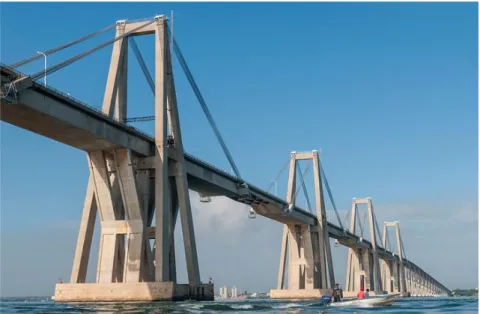
Figure 7 - Maracaibo Bridge (Venezuela,1962) ... 5

Figure 8 - Friedrich-Ebert Bridge (Germany,1967) ... 5

Figure 9 - Pasco-Kennewick Bridge (United States, 1978) ... 6

Figure 10 - Barrios de Luna Bridge (Spain, 1984) ... 6

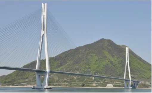
Figure 11 - Tatara Bridge (Japan, 1999) ... 7

Figure 12 - Sutong Yangtze River Bridge (China, 2008) ... 7

Figure 13 - Seven-wire strand ... 8

Figure 14 - Multi-wire helical strand ... 8

Figure 15 – Locked-coil system ... 9

Figure 16 - Parallel -strand cable ... 9

Figure 17 - Cable corroded... 9

Figure 18 - HDPE pipe usage ... 10

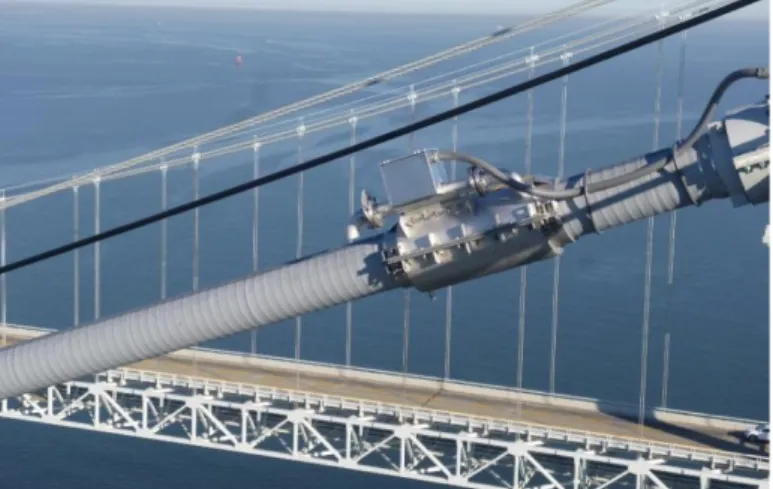
Figure 19 – Dehumidification system applied on the Bay Bridge, United States. ... 10

Figure 20 – Typical components of stay cable anchorage (Freyssint, 2010) ... 11

Figure 21 - Socket for parallel wire strand ... 11

Figure 22 - Internal dumpers: a - Elastomeric (IED), Hydraulic (IED) and Radial (IRD) dampers (Freyssinet, 2014); b – Elastomeric damper; c – Friction damper (VSL, 2002) ... 12

Figure 23 - Anchorage system with eyed bars of the Asashi Kaikyo Bridge ... 12

Figure 24 - Accidental forces for design of cable bridges... 13

Figure 25 - Øresund Bridge SHM sensors (phase II), Denmark-Sweden ... 14

Figure 26 – a) Strain gauges b) accelerometer. ... 15

Figure 27 - Total Station ... 16

Figure 28 - (a) Impulse hammer; (b) eccentric mass vibrator; (c) electrodynamic shaker over three load cells; d) impulse excitation device for bridges. ... 17

Figure 29 - Forced vibration tests: (a) Tatara cable-stayed bridge; (b) Yeongjong suspension bridge; (c) high force shaker ... 18

Figure 30 - (a) Force balance accelerometers; (b) multichannel data acquisition and processing system for ambient vibration tests; (c) strong motion triaxial seismograph ... 19

Figure 31 - Stress-ribbon footbridge at the FEUP Campus. ... 19

Figure 32 - Edgar Cargoso bridge,1982. ... 21

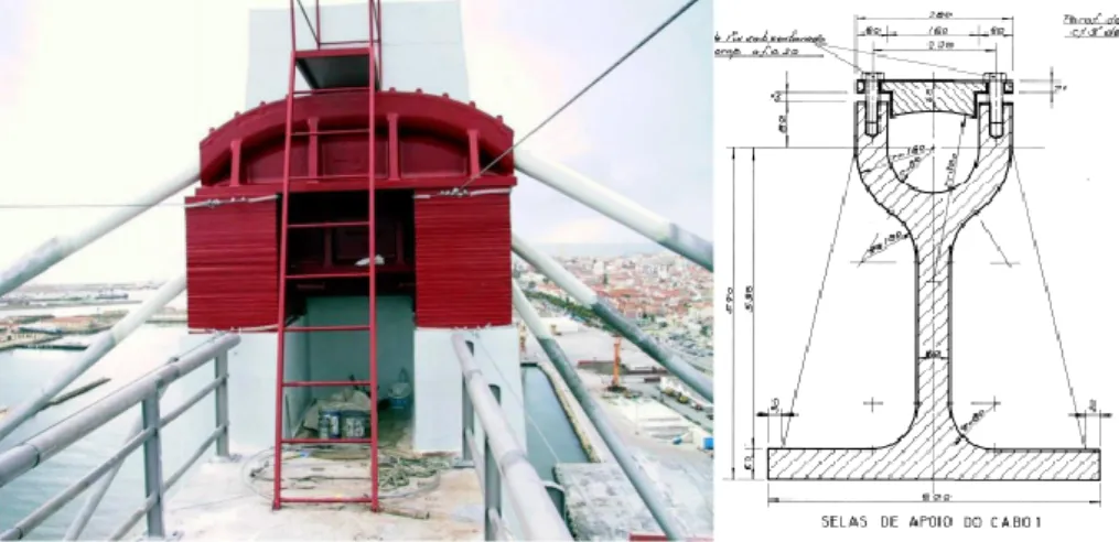
Figure 33 - General view from the saddles arrangement and the design. ... 22

Figure 34 - Deck cross section ... 22

Figure 35 - Deck view ... 23

Figure 36 - Pylon view and geometry ... 23

Figure 37 - Pylon base structure ... 24

Figure 38 - Edgar Cargoso Bridge 3D model ... 25

Figure 39 - Link element variations ... 27

Figure 40 - Releases at the deck bar elements... 27

Figure 41 - Link between the steel deck and the concrete slab ... 28

x

Figure 43 – Pin bearing in the pylon zone... 29

Figure 44 - Suspenders at the edge of the deck ... 29

Figure 45 - Carriageway width ... 31

Figure 46 - Load Model 1 (LM1) ... 31

Figure 47 – Traffic load model 1 distribution ... 32

Figure 48 - Cable tension influence lines ... 33

Figure 49 - Moment influence line ... 33

Figure 50 - Edgar Cargoso bridge location ... 34

Figure 51 - Application of the wind force along the z direction, Fz(ze). ... 37

Figure 52 - Seismic zones for continental Portugal according to the action type. ... 41

Figure 53- SAP2000 response spectrum by the Eurocode 8. ... 45

Figure 54 - Mode shapes for the Edgar Cardoso Bridge ... 51

Figure 55 - Bridge axial load diagram ... 52

Figure 56 - YY bending moment diagram for the bridge deck (Dead load case). ... 52

Figure 57 - Structure displacement (Dead load case). ... 53

Figure 58 - LM4 distribution for the damage analysis ... 56

Figure 59 - Members analyzed in the damage scenarios ... 56

Figure 60 - Cables where the damage was applied ... 57

Figure 61 - Cable affected by the damage scenario 1 (loss on the long cable) ... 59

Figure 62 - Cable affected by the damage scenario 2 (loss on the medium cable) ... 63

xi

GRAPHICS INDEX

Graphic 1 - Transversal Influence Line ... 32

Graphic 2 - Force coefficient cfx,0 for bridge decks (NP EN 1991-1-4, 2019) ... 37

Graphic 3 - Force coefficient to rectangular sections with sharp edges ... 38

Graphic 4 - Boundary effect coefficient ψλ ... 39

Graphic 5 - Response spectrum shape ... 42

Graphic 6 - Seismic behavior factor ... 44

Graphic 7 - Probabilistic approach for load and resistance definition ... 46

Graphic 8 - Recommended values of ψ factor ... Erro! Marcador não definido. Graphic 9 - Example of a damage scenario done for a medium cable ... 58

Graphic 10 - Axial load variation for damage scenarios 1 (loss of long cable on the West side) ... 60

Graphic 11 - Variation of stress for the damage scenario 1 (loss of long cable) ... 60

Graphic 12 - Variation of displacement for the damage scenario 1 (loss of long cable) ... 61

Graphic 13 - Axial load variation for damage scenario 2 (loss of medium cable) ... 64

Graphic 14 - Variation of stress for the damage scenario 2(loss of medium cable)... 64

Graphic 15 - Variation of displacement for the damage scenario 2 (loss of medium cable). ... 65

Graphic 16 - Axial load variation for damage scenarios 3 (loss of short cable). ... 67

Graphic 17 - Variation of stress for the damage scenario 3 (loss of short cable) ... 67

Graphic 18 - Variation of displacement for the damage scenario 3 (loss of short cable) ... 68

Graphic 19 - Axial Force variation for the damage scenario 4 (uniform loss) ... 70

Graphic 20 - Stress variation in the cables for the damage scenario 4 ... 71

xiii

TABLES INDEX

Table 1 - Section properties ... 25

Table 2 - Other permanent loads ... 30

Table 3 - Terrain category and terrain parameters ... 35

Table 4 - Average wind velocities ... 36

Table 5 - Peak velocity pressure ... 36

Table 6 - Force coefficients applied to the bridge deck ... 37

Table 7 - Boundary effect determination values ... 38

Table 8 - Pressure coefficient for cylinders with circular cross-section ... 39

Table 9 - Structural coefficient (cscd) calculation ... 40

Table 10 - Wind force values and coefficients ... 40

Table 11 - Wind force value applied to the z direction on the deck ... 40

Table 12 - Maximum base ground acceleration ... 42

Table 13 - Response spectrum parameters for soil type B ... 43

Table 14 - Maximum values of the behaviour factor q (EN 1998-2:2005+A2:2011) ... 44

Table 15 - Shear reactions for seismic action... 45

Table 16 - Indicative design working life ... 46

Table 17 - Recommended values for γ factor ... 49

Table 18 - Deck self-weight verification ... 49

Table 19 - Stay's axial forces... 50

Table 20 - Comparation of the natural frequencies ... 51

Table 21 - Axial forces on the main span cables ... 52

Table 22 - Pylon section resistance analysis ... 53

Table 23 - Axial forces on a medium cable of the main span after area reduction of the large cable... 55

Table 24 – Cables identification ... 60

Table 25 – Displacement points identification ... 61

Table 26 - Displacements on the tower top for the damage scenario 1 (loss of long cable). ... 62

Table 27 - Modal variation for the damage scenario 1(loss of long cable) ... 62

Table 28 - Variation of stress in the double "I" section for the damage scenario 1 (loss of long cable). ... 63

Table 29 - Variation of stress in the pylon section for the damage scenario 1(loss of long cable). ... 63

Table 30 - Displacements at the tower top for the damage scenario 2 (loss of medium cable). ... 65

Table 31 - Modal variation for the damage scenario 2 (loss of medium cable) ... 65

Table 32 - Variation of stress in the double "I" section for the damage scenario 2 (loss of medium cable). ... 66

Table 33 - Variation of stress in the pylon section for the damage scenario 2(loss of medium cable). 66 Table 34 - Displacements on the tower top for the damage scenario 3 (loss of short cable). ... 68

Table 35 - Modal variation for the damage scenario 3 (loss of short cable) ... 68

Table 36 - Variation of stress in the double "I" section for the damage scenario 3 (loss of short cable) ... 69

Table 37 - Variation of stress in the pylon section for the damage scenario 3 (loss of short cable) ... 70

Table 38 - Displacements at the tower top for the damage scenario 4 (uniform loss). ... 71

Table 39 - Modal response variation for the damage scenario 4 (uniform loss). ... 72

Table 40 - Variation of stress in the double "I" section for the damage scenario 4 (uniform loss). ... 72

Table 41 - Variation of stress in the pylon section for the damage scenario 4 (uniform loss). ... 73

Table 42 - Variation of stress in the cables most affected in each damage scenario. ... 73

xiv

Table 44 - Displacement variation for each damage scenario. ... 74

Table 45 - Displacements on the tower top for the all the damage scenarios. ... 74

Table 46 - Variation in the vibration modes for different damage scenarios ... 75

Table 47 – Stress variation for the double “I” beam ... 75

1

1

INTRODUCTION

1.1 FRAMEWORK

Cable-stayed bridges have become a popular solution to overcame large spans, since they combine an economical and aesthetical advantages for certain constructed spans. In the past half-century, the developments in construction technics, new high-strength materials, and computer technology for structural analyses were fundamental for the diffusion of this structural technique.

Nowadays, the biggest concern about old cable-stayed bridges is the integrity of the cable stays. As these elements are mainly made of high-strength steel, they are very susceptible to suffer corrosion during the bridge lifetime. As the substitution of a stay could be economically inviable, to ensure a proper protection and maintenance is fundamental for the correct functionality of the bridge. According to that, engineers are focused on the structural health monitoring (SHM). This technique is based on the installation of measurement devices to collect data from the structure that can help professionals anticipate some problematic event.

In Portugal, the Edgar Cardoso Bridge is the first cable stayed bridges in the country in its type, opening to traffic in 1982. This structure was designed by the engineer and professor Edgar Cardoso, responsible for other beautiful landmarks around the world and recognized as one of the world’s greatest structural engineers. Unfortunately, nowadays the bridge suffers from some corrosion issues on the cables and has been the object of rehabilitation works and monitoring processes.

1.2 OBJECTIVES

In the contest exposed in the last section, the objectives of this work are:

▪ To develop a finite element model of the structure based on reliable measurements made on the structure.

▪ To simulate damage scenarios that represent the loss of cross section due to corrosion. ▪ To identify the elements that are more sensitive to failure.

▪ To identify which parameters are more influenced by cable loss, so that they can be used as a guideline for further monitoring process.

2

2

STATE-OF-THE-ART

2.1 CABLE-STAYED BRIDGES –HISTORICAL REVIEW

Since old civilizations, the application of cables to support loads has been a popular technique. At the seventeenth century a bridge proposed by Verantius (Italy,1617) was one of the first projects to include inclined stays to support the deck. In the following years Löscher (Germany,1784) also proposed a system of inclined stays very similar to those used nowadays [4].

In 1823, a bridge conceived by Marc Seguin characterized the first use of draw iron wires. This solution had problems related with the durability, since there was no efficient method to prevent corrosion at that time. In alternative, some engineers used pin connected eye-bars in chains as the main load-carrying elements. This system was applied in remarkable structures across the European continent. One of the classic examples is the Albert Bridge (Figure 1) in London, finished in 1873 this bridge is composed by a mixed system of cable stays and suspension [1].

Figure 1 - Albert Bridge (London, 1873)

At the beginning of the nineteenth century wrought iron bars, and later steel wires, with a reliable tensile strength were developed and become an interesting option to be used as inclined stays. But in the early cable-stayed bridges it was very difficult to find an even distribution of the load between all cables. Moreover, imperfections during fabrication and erection could easily lead to a structure where some stays were slack, and others overstressed. The stays were generally attached to the girder and pylon by pinned connections that did not allow a controlled tensioning [1]. By that time, several cable-stayed bridges were proposed and constructed. However, because of the problems faced due to

3

misunderstanding of structural behaviour and construction process, some failures occurred. The Dryburgh Bridge (England, 1817) (Figure 2) and the bridge over the River Saale (Germany, 1824) (Figure 3) are examples of these structural failures. Therefore, for some decades, the uncertainty about cable-stayed bridges lead engineers to consider suspension bridges instead [5].

Figure 2 - Dryburgh Bridge (England, 1817)

Figure 3 - Bridge over the River Saale (Germany, 1824)

In the middle of the 19th _{century cable-stayed systems started to be implemented in several suspension}

bridges as a complementary form to increase global stiffness and the stability against wind actions. At that time, a huge development in construction of suspension bridges was accomplished. The Brooklyn Bridge (Figure 4) opened in 1883, designed by John A. Roebling with main span of 486 m, was the first to use steel cables instead of iron and is the most notable exemplar of these hybrid systems. In the United States, J. Roebling was also responsible for other structures with the same characteristics as the Ohio River Bridge (1867) and Niagara Falls railway Bridge (1855) [5].

4

During the World War II the number of bridges destroyed in West Germany reached, approximately, 15000 [6]. This fact created a necessity to develop innovative solutions to rebuild these structures in a short time. The cable-stayed system emerged as an efficient manner to combine quick erection, aesthetic qualities, and comparatively low costs. Soon, this technique became recognized as an alternative to the classical bridge types, as suspension and arch systems, for medium spans (150-300m) [5].

However, it was in Sweden that the first modern cable-stayed bridge considered in the literature was built, in 1955. The Strömsund Bridge (Figure 5) was designed by the German engineer Dischinger, composed by two side spans of 75m and a main span of 183m. The stays were arranged as a pure fan system with cables radiating from the pylon top. The erection of the Strömsund Bridge also marked the beginning of a new era by implementing new structural analysis techniques. This new approach allowed engineers to calculate cable forces throughout the construction period and thereby assuring the efficiency of all cables in the final stage. From that point, a big expansion on cable-stayed bridges has begun [1].

Figure 5 - Strömsund Bridge (Sweden,1955)

Another remarkable structure was the Severins Bridge (Figure 6) completed in 1959 in Cologne, Germany. This bridge is the first application of an A-shaped pylon combined with transversely inclined cables planes. Also, this was the first asymmetrical two-span bridge with pylon at only one of the riverbanks. This bridge is still in use and became one of the most successful bridges of this type [1]. Following the innovative process, the North Elbe Bridge, with a main span of 172m, constituted the first application of single-plane cables was built in 1962 [5].

5

The success of German constructions and the breakthrough in computer-aided analysis in the mid-1960s extended the cable-stayed system to the rest of the world. The globalization reached the Asiatic continent where the Onomichi Bridge (1968) was the first long cable-stayed bridge in Japan with main span of 215 m. Besides, it is good to point that this structure was made with 82% of corrosion-resistant weathering steel [6].

The multi-span Maracaibo Bridge (Figure 7), in Venezuela, designed by Morandi and finished in 1962 is an exemplar of the so-called “first generation” of cable-stayed bridges. These structures were composed by a small number of stay cables, usually 2 to 6 pairs of stays in the main span, separated by a large distance (more then 30m). This conception results in high tensions in the cables and high stress in the anchorage zone. Because of that, complicated anchorages were needed, and several ropes were used to form each stay [5].

Figure 7 - Maracaibo Bridge (Venezuela,1962)

The evolution of new technologies for structural analysis lead to the introduction of multiple-cable systems where each stay is a single prefabricated strand. This system involves a high degree of indeterminacy, impossible to solve by hand, but well reached with the new technology [1]. The first use of this new system was made in the Friedrich-Ebert Bridge (Figure 8) opened in 1967 over the Rhine river in Bonn, Germany. The bridge has a central steel deck that span over 280m supported by 20 stays, on each side, connected to two pylons. The multiple-cable technique increases the flexural stiffness of the deck and reduces the stress concertation, simplifying the anchorages. In addition, the reduction of spacing between cables allow a simpler phased construction by free cantilever [5].

6

By the end of 1970s, a new generation of cable-stayed bridges have been launched. The concept applied for the first time in the Pasco-Kennewick Bridge (Figure 9) in 1978 has a deck entirely supported by the cable-stayed system. The structural behaviour was very different from the other bridges constructed so far. The deck now acts as a compressive chord of a truss hang up to the towers by inclined stays [5]. At this period, the usage of concrete deck was begging to become popular. In 1984, the Barrios de Luna Bridge (Figure 10) built in Spain gave a strong indication that concrete was a competitive material to be used not only in the pylons but also in the deck of cable-stayed bridges [1].

Figure 9 - Pasco-Kennewick Bridge (United States, 1978)

Figure 10 - Barrios de Luna Bridge (Spain, 1984)

At the end of the 20th _{century major achievements in the construction of cable-stayed bridges have been}

made. For the first time a span with more than five hundred meters has been placed. The Skarnsund Bridge (Norway,1991) and the Yangpu Bridge (China, 1993) were the first to break this boundary. However, the greatest realizations were made by the end of the decade with the Normandy Bridge in France (1995) with a main span of 856m and the Tatara Bridge (Figure 11) that opened to traffic in 1999 with the record of 890m in Japan [1].

7

Figure 11 - Tatara Bridge (Japan, 1999)

The first 20 years of the 21st _{century have been marked by a big development of the Asian economy}

driven mainly by China. Consequently, over thirty cable-stayed bridges with main span greater than 500m were made in this short period of time in China. The most notable bridges to refer are:

▪ Sutong Yangtze River Bridge (Figure 11), 2008 – main span of 1088m ▪ Stonecutters Bridge, 2009 – main span of 1018m

▪

Edong Yangtze River Bridge, 2010 – mainspan of 926m

Figure 12 - Sutong Yangtze River Bridge (China, 2008)

The limit of this impressive structures is very uncertain. Today many researchers are developing new techniques and materials to reach spans over more than two kilometres. The implementation of materials such as Fibre-Reinforced Polymer (FRP) is a reality in the civil engineering field and is one of the most promising method to achieve those impressive numbers [7].

2.2 CABLES

2.2.1 CABLE TYPES

Basically, cables are arrangements of high strength steel wires. The wires are assembled to form a strand and later used to shape a cable on site or in the shop. The seven-wire (Figure 13) strand is the simplest form to be found in a cable supported bridge. The wires have, in general, 5mm diameter and tensile

8

strength between 1770 and 1860 MPa. They are normally arranged with a single straight core confined by one level of six wires placed in a helicoidal course [1].

Figure 13 - Seven-wire strand

The multi-wire helical strand, also called spiral strand, is conceived in a similar way to the seven-wire strand. However, this type has multiple wire layers with opposite course directions, as illustrated in Figure 14. As a side effect, when the wires are twisted the total strength drops when compared to the straight element. Approximately, the final strength of a helicoidal strand is 10% lower than the sum of all parallel wires. The nominal modulus of elasticity is also affected by the helicoidal shape of the top layers 15-25% below the value for straight wires. This phenomenon also occurs on the seven-wire strand but with less magnitude [1].

Figure 14 - Multi-wire helical strand

As an alternative to the normal strands there is the locked-coil system. This type of cables is an array of round wires surrounded by an outer layer of special Z-shape wires. The Z-shape wires guarantee a tight surface protecting the interior of corrosion. The final protection against corrosion used to be a surface treatment with painting, nowadays all the wires are galvanized instead. Strands at this system are manufactured in full length and with a diameter range from 40mm to 180mm. Large strands are normally used in cable-stayed bridges with multi-cable systems where every stay is a mono-strand cable [1].

9

Figure 15 – Locked-coil system

However, difficulties in the design of anchorages and protection against corrosion restricted the usage of this types of systems. Today, the main option adopted in several countries is the parallel-strand cable (Figure 16) [3]. In this system seven-wire strands with a protection layer of high-density polyethylene (HDPE) are arranged together in parallel to form the cable. In many cases the stay is surrounded by a cylindrical pipe in order to reduce the drag coefficient due to the grooved surface [1]. Cables of this type can have between 18 and 90 strands with breaking load up to 24 MN [3].

Figure 16 - Parallel -strand cable 2.2.2 CORROSION PROTECTION

Project specifications must guarantee adequate lifetime to the cable stay based on economic conditions. Generally, a 100-year service lifetime period is considered appropriated for suspension and cable-stayed bridges. For this purpose, protection against corrosion is substantial to achieve the required level of durability [8].

In cables composed by many wires the impact of corrosion is more pronounced. Each wire has a small diameter, plus most are inaccessible to direct inspection and maintenance. Thus, voids between wires and the steel material make these cables even more vulnerable to this effect. For example, a cable with a reduction of 1mm in the surface due to corrosion could represent a 64% loss area, a value far from been covered by safety margin [1].

10

Today, as a constructive rule, cable stays should have at least two barriers against corrosion. These two layers are complementary. The internal barrier is applied individually to all wires in the full length of the cable. As a second barrier an external protection should be placed to prevent the internal barrier being consumed. Is very important that the external layer must be water and airtight in both the free length and the anchorage zone.

The internal barrier can be done with metal or non-metal coating. For the metal coating generally pure zinc (galvanization) is used or else zinc-aluminium compound. The quality and the durability of these protections depends on the thickness of the metal coating. Non-metal protection is equivalent to the galvanization, but instead resins or polymers are used.

The external protection used varies with the type of cable stays and with especial requirements of the structure. The most frequently used are some of the following: Stay pipes made of high-density polyethylene (HDPE) (Figure 18), plastic sheath extruded directly on the strand or steel stay pipes made of stainless steel or with protection coatings. Besides, stay pipes also fulfil other functions like mechanical (limiting cable-stay drag), aerodynamics (limiting rain and wind induced instability) and aesthetic (colour) [2].

Figure 18 - HDPE pipe usage

An intermediate cover is also used to avoid humidity inside the core. Generally, wax, grease or resin are placed to fill the blanks. Cement grout was also used in the past, but this method is less effective once cracks due to shrinkage do not create a full tight surface and it is also known that the cement grout can initiate corrosion process. However, another method was found very efficient, to install dehumidifiers to inject dry air inside the cable voids (Figure 19) removing the water needed for the corrosion’s chemical reaction. This system was applied by the first time in the Akashi-Kaikyo Bridge constructed in the late 1980s [8].

11

Even though, none of those solutions can offer a full protection against corrosion. Meaning that the only way to prevent this problem is to provide an additional periodic maintenance in the cables.

2.2.3 ANCHORAGE SYSTEMS

Anchorage systems are crucial for the structure, this elements are responsible to transfer the actions that came from the deck and transfer them to the cables(Figure 20). Special requirements are needed to design this system, especially them to have appropriated mechanical resistance and fatigue resistance [8].

Figure 20 – Typical components of stay cable anchorage (Freyssint, 2010)

A bridge anchor is composed by two main parts: the anchorage head, that is responsible for the load transmission; and the transition zone, where the cable arrangement changes to fit the anchorage system [2]. To anchor parallel-wires strands a special socket was developed in the 1970s, where the wires are displaced through holes in a locking plate at the far end of the socket and provided with button heads to increase the resistance against the slipping of individuals wires. The concavity inside the socket is filled in general with cold cast materials, such as epoxy resin, zinc dust or small, hardened steel balls, in order to reduce fatigue effects.

12

The principal functions that an anchorage must accomplish are listed below [8]: ▪ Properly transfer the loads

▪ Filtering out angular deviation ▪ Possibility of adjustment ▪ Corrosion protection ▪ Removability

Besides, in order to prevent cable vibration internal dampers can be added close by the anchorage element (Figure 22).

Figure 22 - Internal dumpers: a - Elastomeric (IED), Hydraulic (IED) and Radial (IRD) dampers (Freyssinet, 2014); b – Elastomeric damper; c – Friction damper (VSL, 2002)

A variety of anchor types are available, depending on the solution adopted for the structure. In past solutions, using eye-bars and strand shoes were very common, according to the trends of bridge constructions of the time. Recently, the use is focused on standard solutions based on wire cables that allow the maintenance and implementation of devices such as dehumidifiers.

13

2.3 CABLE LOSS

In cable-stayed bridges, damage, or failure of primary structural components such a pylon, deck, or cables, caused by accidental events can lead to the collapse of the entire bridge [9].

The collapse mechanism of the cable stayed bridge is called "zipper-type collapse", in which the first stay snapped due to an excessive increase of stress from an accidental event or loading [10] [11]. Guidelines, such as PTI D-45.1-12 2012 (Post Tensioning Institute, 2005), Eurocode 1 part 1.7, SETRA, recommend considering cable loss scenarios during design phase, with the implementation of a dynamic amplification factor for static loads that doubles the forces applied to the structure in case of failure.

Figure 24 - Accidental forces for design of cable bridges

Furthermore, the bulletin CEB-FIB, 2005, recommends that the design of cable stays for bridges must allow the replacement of these structural members one or more time during the lifetime of the structure. The damage caused by a cable rupture in a cable stayed bridge could lead to a scenario called “progressive collapse” where the rupture of one element leads to a redistribution of loads that overwhelm other members of the structure, and consequently, rupture. In the past, several structures suffered from damage that directed to the progressive collapse or has affected the usability of the bridge [12].

The loss process in the cable cross-section area will initiate the loss of compression in the bridge girder of a cable-stayed bridge. The loss of bracing on the girder leads to an increase in vertical deflections thus inducing high stresses in the longitudinal girder lying in the plane of the cable loss which then transmits to the longitudinal girder of the other plan of the cables. This pattern of collapse is defined as: Instability –type collapse [14].

In addition, loss of cables leads to overloading of the adjacent cables, and then the load carried by these adjacent cables will be re-distributed to other nearby cables termed unzipping which causes a zipper pattern of progressive collapse. Concrete bridge decks and segmental/ non-continuous bridges decks do not experience this type of collapse pattern. Zipper-type collapse is initiated by the failure of one or more tension elements which then redistribute the forces carried by the failed elements to the remaining structure. The sudden failure induces an impulsive load and the remaining structure responds in a dynamic way, leading to stress concentrations in the next elements along the direction transverse to the principal forces in the elements [15].

When designing a structure to limit state conditions, the event of losing a cable is governed by the Ultimate Limit State design while effects such as deflection, cracking, creep, shrinkage etc. are related to the serviceability of the structure. The loss of a major element may not lead to the collapse of the bridge but can lead to slacking of the cables and thus large deflections in the deck or large vibrations in the deck [11]. This invariably reduces the comfort of the bridge users.

When a cable fails the deck can experience vertical displacement, vibration, and flexural/ buckling at the location of the lost cable. If breakage of the cable occurs at different locations, then the deck may

14

experience vertical deformations causing varying uplifts along the deck These varying uplifts of the girder can be used to detect which cables in an existing cable-stayed bridge have broken [16]. In decks with twin cable planes, cable loss along one plane introduces eccentricity in the deck supports, leading to large deflections and with the live loads present is a potential cause of instability [17].

2.4 STRUCTURAL MONITORING

Structural health monitoring (SHM) systems are extensively adopted to estimate the behaviour of structures under ambient and forced vibrations in a laboratory environment or in the field and used to monitor structures under other excitations such as earthquakes, traffic, gusts, or live loading [18]. The SHM can play a vital role in the maintenance and health evaluation of cable-supported bridges. In the past three decades, it has been used primarily and effectively for damage detection in bridges, especially where there is some doubt about the performance of a particular design or when the expected loading has been difficult to quantify in the design stages of the bridge. Storms, earthquakes, floods, and accidents are examples of this type of loading. SHM can be used not only for the detection of damage though. It can also be used for the quantification of the severity of damage and the locations of damage [2].

Developments have lead researchers and engineers to use existing SHM techniques and hardware for new purposes. It is not uncommon for SHM equipment to be used temporarily and selectively during the construction of a large bridge to evaluate the construction sequence and to provide data that will help improve the completion of not only the particular bridge, but also other similar bridges in future. The SHM became an important tool to evaluate the need for the retrofit of bridges with the goal of a fail-safe bridge design. In all cases SHM is being used to help close the gap between the theoretical evaluation and the real-life performance of bridges [2].

The measurements on the structure are also important to modal identification of bridges and other civil structures. This information is important for the validation of finite-element models used to predict static and dynamic structural behaviour either at the design stage or at rehabilitation. After appropriate experimental validation, finite-element models can provide essential baseline information that can subsequently be compared with information captured by long-term monitoring systems to detect structural damage [20]. An example of this is the Øresund Bridge (Figure 25), where engineers decided to measure both the static and the dynamic response of the bridge to passing vehicles and trains and the dynamic response of the stay cables to wind. Furthermore, strain gauge measurements were found to be of interest at the locations of maximum expected strain, around the cable outriggers and at several locations on the bottom chord of the bridge. More specifically, the bridge is fitted with 22 triaxial force balance accelerometers, 19 strain gauges, several thermometers to correlate the strain gauge measurements with the variations in temperature, and two bi-axial ultrasonic anemometers to measure the oncoming wind velocities and turbulence intensities [2].

15

The most common sensors used for bridge monitoring are strain gauges and accelerometers (Figure 26). Each respectively assists in the understanding of the bridge’s static and dynamic response to traffic and environmental loading. Based on these measurements, a more accurate evaluation of the structural performance can be made, together with more precise fatigue calculations. The dynamic response of the bridge can also be evaluated globally or locally, often with the goal of determining structural properties that cannot be theoretically evaluated with any great degree of accuracy. These might include structural damping, cable tensions or bridge mode shapes and frequencies [2].

Figure 26 – a) Strain gauges b) accelerometer.

Modern accelerometers, as shown in the Figure 26 are well suited for measurements in the range of 0-50 Hz and are virtually insensitive to high-frequency vibrations. They have contributed significantly to the success of ambient vibration tests. In such tests, the structural ambient response is captured by one or more reference sensors at fixed positions and with a set of roving sensors at different measurement points along the structure and in different setups. The number of points used is conditioned by the spatial resolution needed to characterize appropriately the shape of the most relevant modes of vibration (according to preliminary finite element modelling), while the reference points must be far enough from the corresponding nodal point. This system can be implemented on a normal PC. Some data acquisition and processing systems, specifically designed for ambient vibration tests, are already available [20]. Alternative sensors include inclinometers, relative displacement transducers and, more recently, laser displacement transducers and Global Positioning System (GPS) equipment. Relative displacement transducers are often used to measure local deformations or bearing and expansion joint movements. Laser transducers offer the same capability, but without the need for contact between the measured surfaces. GPS equipment works relatively well in providing mean horizontal displacements, but not so well in providing vertical displacements. The combined Total Station (TPS) (Figure 27) with powerful Laser Doppler Velocimetry (LDV) measurement. With this technology, measurements can be made on a bridge from a distance of up to 2 km with a very high degree of accuracy. A precise TPS can scan a large bridge quickly to allow a powerful laser to measure variations in the position of a bridge for any point on the bridge that the laser is in contact with. Shifts in modal properties, local distortions or global displacements can readily be logged [2].

The most common instrumentation programs are of short duration. Static measurements are performed during the bridge construction and at spaced time intervals after completion, while dynamic measurements are performed at the end of construction. Some sensors are however left at the bridge, which trigger particular events, like earthquakes and severe wind condition, or send alarm signals

16

whenever excessive vibrations or displacements are attained. More sophisticated SHM perform continuous measurements, storing statistical information and particular records. These systems incorporate communications with a Central Station (Figure 27), which may be located several hundreds of kilometres away, and from where specific commands concerning the signal acquisition and processing can be issued, such as data transfer or change of the signal acquisition parameters [5].

Figure 27 - Total Station

In addition to this measurement’s systems test can be done to measurement of the structural response. The Forced Vibration Testing (FVT) techniques employed in Civil Engineering structures constitute straight applications of the so-called Modal Analysis Techniques, which were born in the areas of Mechanical and Aeronautic Engineering some decades ago. These techniques are based on the application of a controlled excitation, and measurement of the response at a set of locations. From the set of excitation and response time histories, estimates of Frequency Response Functions (FRF’s) or of Impulse Response Functions (IRF’s) can be obtained (for frequency or time domain analysis, respectively) and System Identification algorithms applied, in order to extract the most relevant dynamic parameters of the structure, i.e., the natural frequencies, vibration modes and damping coefficients[18]. The instrumentation systems employed for dynamic testing of structures comprehend the following main components:

▪ a subsystem for excitation.

▪ a subsystem for measurement of applied forces and responses.

▪ a data acquisition modulus, for control of excitation, and for recording and analysing the measured data.

In small and medium-size structures, the excitation can be induced by an impulse hammer (Figure 28a) similar to those currently used in mechanical engineering. This device has the advantage of providing a wide-band input that can stimulate different modes of vibration. The main disadvantages are the relatively low frequency resolution of the spectral estimates (which can preclude the accurate estimation of modal damping factors) and the lack of energy to excite some relevant modes of vibration. Due to this problem, some laboratories have built special impulse devices specifically designed to excite bridges

17

(Figure 28b). An alternative, also derived from mechanical engineering, is the use of large electrodynamic shakers (Figure 28c), which can apply a large variety of input signals (random, multi-sine, etc.) when duly controlled both in frequency and amplitude using a signal generator and a power amplifier. The shakers have the capacity to excite structures in a lower frequency range and higher frequency resolution. The possibility of applying sinusoidal forces allows for the excitation of the structure at resonance frequencies and, consequently, for a direct identification of mode shapes.

Figure 28 - (a) Impulse hammer; (b) eccentric mass vibrator; (c) electrodynamic shaker over three load cells; d) impulse excitation device for bridges.

This process is identified as input-output modal identification methods whose application relies either on estimates of a set of frequency response functions (FRFs) or on the corresponding impulse response functions (IRFs), which can be obtained through the inverse Fourier transform. These methods attempt to perform some fitting between measured and theoretical functions and employ different optimization procedures and different levels of simplification. Accordingly, they are usually classified according to the following criteria:

▪ Domain of application (time or frequency)

▪ Type of formulation (indirect or modal and direct)

▪ Number of modes analysed (SDOF or MDOF – single degree of freedom or multi degree of freedom)

▪ Number of inputs and type of estimates (SISO, SIMO, MIMO, MISO – single input single output, single input multi output, multi input multi output, multi input single output).

The main problem associated with forced vibration tests on bridges, buildings, or dams is the difficulty in exciting the most significant modes of vibration in a low range of frequencies with sufficient energy and in a controlled manner. In very large, flexible structures like cable-stayed or suspension bridges, the forced excitation requires extremely heavy and expensive equipment usually not available in most

18

dynamic labs. The Figure 29 shows the impressive shakers used to excite the Tatara and Yeongjong bridges for dynamic tests [20].

Fortunately, recent technological developments in transducers and A/D converters have made it possible to accurately measure the very low levels of dynamic response induced by ambient excitations like wind or traffic. This has stimulated the development of output-only modal identification methods. Therefore, the performance of output-only modal identification tests became an alternative of great importance in the field of civil engineering. This allows accurate identification of modal properties of large structures at the commissioning stage or during their lifetime without interruption of normal traffic.

Figure 29 - Forced vibration tests: (a) Tatara cable-stayed bridge; (b) Yeongjong suspension bridge; (c) high force shaker

In such tests, the structural ambient response is captured by one or more reference sensors at fixed positions and with a set of roving sensors (Figure 30) at different measurement points along the structure and in different setups. The number of points used is conditioned by the spatial resolution needed to characterize appropriately the shape of the most relevant modes of vibration (according to preliminary finite element modelling), while the reference points must be far enough from the corresponding nodal points.

19

Figure 30 - (a) Force balance accelerometers; (b) multichannel data acquisition and processing system for ambient vibration tests; (c) strong motion triaxial seismograph

The correlation of modal parameters can be analysed both in terms of identified and calculated natural frequencies and by corresponding mode shapes using correlation coefficients or MAC (modal analysis criteria) values. Beyond that, modal damping estimates can be also compared with the values assumed for numerical modelling. This type of analysis has already been developed for the Vasco da Gama and Luiz I bridge with excellent results and has been applied over the last years at several bridges in Portugal. The accurate identification of the most significant modal parameters based on output-only tests can support the updating of finite-element models, which may overcome several uncertainties associated with numerical modelling. Such updating can be developed based on a sensitivity analysis using several types of models and changing the values of some structural properties to achieve a good match between identified and calculated modal parameters.

An example of the application of this procedure is the stress-ribbon footbridge at the FEUP Campus where it was studied the dynamic behaviour of the bridge (Figure 21). For this purpose, different finite elements models were developed in order to achieve a good correlation between identified and calculated natural frequencies and mode shapes.

21

3

STRUCTURE DESCRIPTION

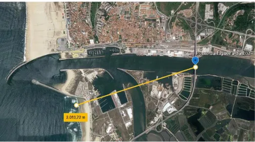
The object of study of this work is the Edgar Cardoso Bridge (Figure 32) a Portuguese bridge that opened to traffic in 1982 as the first cable-stayed bridge in the country. This bridge is located in the city of Figueira da Foz, about 160km north from Lisbon, and is composed by two side spans with length of 90m and a main span 225m long. This structure was designed by Prof. Edgar Cardoso and constructed by OPCA.

Figure 32 - Edgar Cardoso bridge,1982. 3.1 STAYS

Arranged in a fan system, the cables are made of steel wires with a tensile strength of 1600-1800 MPa. Every cable is anchored end to end at the deck spaced by 30 m and passing through saddles placed on the top of the mast. The stays are formed from 900, 540 and 390 wires, respectively, from the longer to the shorter cable.

22

Figure 33 - General view from the saddles arrangement and the design. 3.2 DECK

The deck is composed by steel I-girders supporting a concrete slab of 0.13 to 0.2m thick. With a total width of 20m, the deck is constituted by 2 traffic lanes of 7.5m and a pedestrian lane of 2m on each side ( Figure 34).

Figure 34 - Deck cross section The main steel parts that constitute the deck (Figure 35) are:

▪ Main girders conceived by pairs of I-section on both sides with: 2065mm height, 25mm thick bottom flange, 40mm thick top flange and web thick of 20mm.

▪ Four HE 600 A longitudinal girders spaced of 3.20m.

▪ Transversal I-beams with 15.5 span every 10 m following the respective geometry: 2050mm high, 25mm thick flanges and web thick of 16mm.

▪ The top flange of the main girders is braced by a ½ HE 360 A section diagonal member. The steel used in the main girders is a S355 grade and for all the other members were used S235.

23

Figure 35 - Deck view 3.3 PYLON

The bridge has two concrete pylons with 84.4m to support the vertical reactions, as shown in the Figure 36. Each pylon has four concrete legs with hollow squared section. These legs are inclined elements connected at the top by a transversal beam and under the deck by a concrete laminate plate. The concrete used in the pylon, as well as in the deck, has a compression resistance varying in the range from 56 to 72.3 MPa, being characterized by an inspection made in 1998 by Eng. Júlio Appleton and Eng. Armando Rito.

Figure 36 - Pylon view and geometry

At the base level, the towers are supported by four circular hollow piles with an exterior diameter of 5 meters and wall thickness of 0,40m. The pile blocks are interconnected by prestressed I-sections concrete beams (Figure 37).

24

Figure 37 - Pylon base structure

3.4 DAMAGE IDENTIFICATION

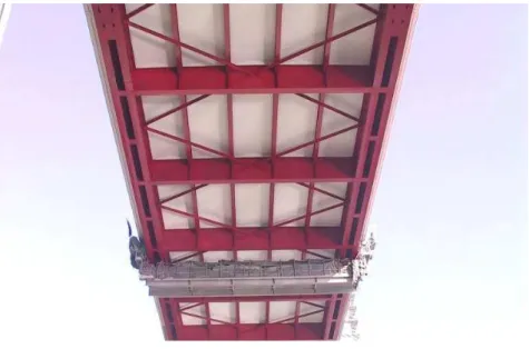
During the last two decades the Edgar Cardoso Bridge have been object of rehabilitation works and monitoring process. Figure 38shows some points of corrosion identified in the anchorage zone of one of the cables during one of the monitoring works done in the bridge.

Figure 38 - Corrosion identify on the Edgar Cardoso Bridge [22]

In this context, one of the main objectives of this work is to characterize the damage level that this structure can support. To identify the structural behaviour of the bridge and through which mechanism it will be possible to determinate the development of a more pronounced damage a Finite Element Model (FEM) will be done. The next chapter will discuss the techniques implemented in the modelling process and the corresponding validation.

25

4

STRUCTURAL MODELLING

4.1 MODELLING PROCESS

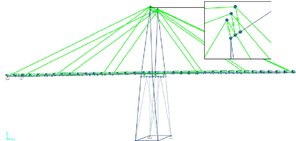
To analyse the structural behaviour of the Edgar Cardoso Bridge a complete 3D model was done using the SAP2000 software. Figure 39 represents a perspective of the final model.

Figure 39 - Edgar Cardoso Bridge 3D model

The modelling process followed the original project made by Eng. Edgar Cardoso [23] and latter information from the rehabilitation report [23] done by the Eng. Julio Appleton, Eng. Armando Rito and their collaborators.

To simulate the steel deck and the pylon, bar elements were used. This type of elements requires section input that were taken from the rehabilitation report mentioned earlier in this section. In addition to all the geometrical properties of the section, it is also mandatory to input the material properties. Table 1 - Section properties shows all the sections and material properties applied to these elements.

Table 1 - Section properties

Section Properties

(mm)

Four longitudinal beams HE 600 A

Area: 22645.8 mm² Centroid: X: 150 mm Y: 295 mm Radii of gyration: X: 386.50 mm Y: 165.76 mm Principal moments and X-Y directions about centroid: X-X:141208 x10⁴ mm⁴ Y-Y: 11271 x10⁴ mm⁴ Weight per meter: p2=78.5x2.265e-2=1.8 kN/m Steel S235 25 540 25 13 R27

26

(mm)

Two double "I" beams in the extreme edge of the steel deck. Area: 145000 mm² Centroid: X: 750 mm Y: 1131.8 mm Radii of gyration: X: 1384.14 mm Y: 906.75 mm Principal moments and X-Y directions about centroid: X-X: 9205291 x10⁴ mm⁴ Y-Y: 3765639 x10⁴ mm⁴ Weight per meter(plus 20% to include connections): p1=1.2x78.5x0.145=6.8 kN/m Steel S355 (mm) Transversal beams Area: 57000 mm² Centroid: X: 250 mm Y: 1025 mm Radii of gyration: X: 1298 mm Y: 265 mm Principal moments and X-Y directions about centroid: X-X: 3615886 x10⁴ mm⁴ Y-Y: 45133 x10⁴ mm⁴ Weight per meter: p3=78.5x0.057=4.5 kN/m

Steel S235

(mm)

1/2 HEA 360 braces

Weight per meter - p4=0.56 kN/m Steel S235

(m)

Concrete pylon leg cross section

Area: 4.37 m² Centroid: X: 1.00 m Y: 0.80 m Radii of gyration: X: 0.9024 m Y: 1.1322 m Principal moments and X-Y directions about centroid: X-X: 0.762 m4 Y-Y: 1.231 m4 Concrete C55/60 300 175 17,5 R27 500 500 500 40 200 0 25 500 2000 25 500 25 16 2.00 0.35 1.60

27

The next step, after modelling all these elements, is to set the connectivity properties between the elements. In the software it is possible to do it in two ways: connection by nodes or link elements. The first method is used when bars have a common point, then it is possible to introduce releases by changing the element properties. When elements have different position in the space, then the connectivity is made by links. A link (Figure 40) object connects two joints, i and j, separated by length L, such that specialized structural behaviour may be modelled. Linear, nonlinear, and frequency-dependent properties may be assigned to each of the six deformational degrees-of-freedom (DOF) which are internal to a link, including axial, shear, torsion, and pure bending.

Figure 40 - Link element variations

In this project all the HEA600, transversal beams and braces were modelled in the same plane and then connected by a common node. This process requires offset application to correct the elements position. On this group of beams the connectivity properties were set so they work as pinned elements, so free rotation releases at the transversal XY axis were set.

In order to have the exact length of the cables, the double “I” beams were modelled exactly in their centroid position. Therefore, the transversal beams were connected to the double “I” beams by links with fixed displacement and free rotation. In the Figure 41, all the deck connections and links are exposed.

Figure 41 - Releases at the deck bar elements

The deck is also composed by a concrete slab with variable height between 0.13m and 0.20m. To model the slab shell objects were used, but to this type of elements the software only allows a constant height to be set, so an average height was input to this slab. Since connectors were not used to join the slab to

28

the steel deck, it was assumed that there is no relevant participation of the concrete slab in the bending resistance of the deck, so it is expected that the height simplification will not have a great influence in the final model. As a preliminary assumption, the connectivity between the shell and the steel frames was made with free longitudinal displacement links and free rotations about the longitudinal and transversal axes of the bridge(Figure 42).

Figure 42 - Link between the steel deck and the concrete slab

The pylons are a less complex structure with no need for links or releases, they have four elements: columns, concrete laminate plate, top beam, and foundations. The four columns have the same section, that is described in the Table 1, and were assembled as bar elements. The concrete laminate plate has a thickness of 30 centimetres and was modelled as a shell element. The top beam has also been modelled as a bar element and the cross section is listed in the Table 1. Foundations were characterized by fixed supports that were applied on each pylon leg.

To support the deck 24 stays are anchored between the two “I” sections that compose the main longitudinal beam. In the real structure each two cables of the same plan are one single object that goes from deck anchorage in the central span to deck anchorage in the side span passing through a saddle on the top of the tower. However, in the 3D model cables are objects defined by a two-point line, so it is impossible to make a single object such as the real element. To simulate the correct cable behaviour a link element with free longitudinal displacement (Figure 43) was applied at the saddle position, in order to constrain vertical and transversal cable and tower movements, but allowing relative longitudinal displacements, to simulate the possible sliding and distribution of the force according to the applied loads.

29

In addition, 16 pinned bearings, eight on each tower, also support the deck of the bridge. The pin bearing allows rotation in one direction. In Figure 44, a copy from the original project shows a detail view from the element. To model this, support a link was used with free rotation along the longitudinal direction, but fixed about the transversal axis.

Figure 44 – Pin bearing in the pylon zone.

The simply supported deck segment in the central part of the bridge originates a non-symmetrical loading (with respect to the tower) of the deck which cannot be balanced, since the other two parts of the bridge are symmetrical. In order to transfer the added load to the supports, two vertical anchors to the transition columns have been placed on each side of the bridge (Figure 45). To simulate their effect, two supports with only vertical displacement restriction were set on both edges of the double “I” beams, as shown in the Figure 45.

Figure 45 - Suspenders at the edge of the deck 4.2 LOAD CASES

The next step after modelling all the elements was to set the load cases. For this work, the load definition was based on the Eurocode 1 for wind [26] and traffic loads [27] and Eurocode 8 for seismic action and additional information available on the rehabilitation report [23].

30

4.2.1 DEAD LOAD

The Edgar Cardoso bridge has two main materials, concrete and steel. For the concrete members, a specific weight of 25 kN/m³ was considered that includes the reinforcement and 78,5 kN/m³ was used for the steel parts. The software automatically considers the self-weigh of the elements modelled, so it was not necessary to add a load for this case. In addition, the bridge is also composed by non-structural elements and their load must be assigned to the elements for latter analysis. The values adopted to calculate the extra permanent load are systematized in Table 2 and were extracted from the original project of this bridge and from the rehabilitation report [23]:

Table 2 - Other permanent loads

Description Load (kN/m)

Parapets 6,0

Kerb 3,2

Footway floor 8,8

Central reservation floor 1,6

Pavement 18,8

Guard rails 5,0

Pipelines 5,0

Total 48,4

To reach these values a simple calculation was processed, multiplying the elements area by their self-weight. However, for this work the total load was equally distributed on the bridge deck. The results of this procedure are exposed bellow.

Linear load (L.L) – 48,4 kN/m ≈ 50 kN/m

Distributed load = L.L/Deck width = 50/20 = 2,50 kN/m²

However, after the validation that will be discussed latter on this chapter, was noticed that an increment on the self-weight was necessary to reach the axial forces measured on site on the cables. For this purpose, a permanent load of 3,5 kN/m² was applied to the deck on the FE model.

4.2.2 TRAFFIC LOAD

The Eurocode 1 part 2 (NP EN 1991-2) establishes the actual traffic load to be used for bridge design [27]. Following the European standard, there are four load models that can be applied to the structure. These are the following:

▪ Load Model 1 (LM1) - Concentrated and uniformly distributed loads, which cover most of the effects of the traffic of lorries and cars. This model is recommended to general and local verifications.

▪ Load Model 2 (LM2) - A single axle load applied on specific tire contact areas which covers the dynamic effects of the normal traffic on short structural members. Used mainly to local verifications.

31

▪ Load Model 3 (LM3) - A set of assemblies of axle loads representing special vehicles (e.g. for

industrial transport) which can travel on routes permitted to abnormal loads. Applied for general and local verifications.

▪ Load Model 4 (LM4) - A crowd loading, intended only for general verifications.

For this work only the LM1 and the LM4 were used since only global verifications will be conducted. These models are applied along the carriageway width that is defined by the standard. The Edgar Cardoso bridge has a permanent reservation area in the middle of the deck, so the carriageway is divided in two pieces as shown in the figure (Figure 46)

Figure 46 - Carriageway width

The carriageway is divided into lanes were the tandem systems are assigned. Figure 34 explains this distribution for the Load Model 1.

Figure 47 - Load Model 1 (LM1)

To apply the load on the structure deck, it is necessary first to calculate the transversal influence line so that the load is arranged to produce the maximum stresses required for a future analysis. To calculate the influence line of one of the main beams the Courbon method was adapted, which is based on the stiffness distribution of the girders. The equation 1 was used to construct this influence line.

𝑅(𝑗) = 𝑘𝑗 ∙ ( 1

∑ 𝑘𝑖+ 𝑥𝑗

∑ 𝑘𝑖∙𝑥𝑖²∙ 𝑥) (1)