Canonical Correlation Analysis in variable
aggregation in DEA
Armando B. Mendes
†Veska Noncheva
‡Emiliana Silva
‡† CEEAplA e Universidade dos Açores ‡ CEEAplA e Universidade dos Açores [email protected] [email protected]
www.uac.pt/~amendes
‡ University of Plovdiv “Paisii Hilendarski”
Bulgaria
Abstract
In this paper we will document the application of canonical correlation analysis to variable aggregation using the correlations of the original variables with the canonical variates. A case study, about farms in Terceira Island, with a small data set is presented. In this data set of 30 farms we intend to use 17 input variables and 2 output variables to measure DEA efficiency. Without any data reduction procedure several problems known as “curse of dimensionality” are expected. With the data reduction procedures suggested it was possible to conclude quite acceptable and domain consistent conclusions.
Resumo
Neste trabalho documenta-se a aplicação de análise de correlações canónicas à agregação de variáveis em DEA, usando as correlações entre as variáveis originais e os componentes canónicos extraídos. É apresentado um caso de estudo que utiliza um pequeno conjunto de dados sobre explorações agrícolas na ilha terceira. Neste conjunto de 30 explorações agrícolas pretende-se usar 17 variáveis de input e 2 de output para avaliar a eficiência usando DEA. Sem qualquer redução de dados, vários problemas conhecidos como “praga da dimensionalidade” seriam esperados. Com os procedimentos sugeridos foi possível obter resultados razoáveis e de acordo com o conhecimento de domínio actual.
Keywords: DEA, CCA, feature selection and extraction
1 Introduction
Data Envelopment Analysis (DEA) is becoming an increasingly popular management tool. The task of the DEA is to evaluate the relative performance of units of a system. It has useful applications in many evaluation contexts and across several disciplines. Is not a problem solution technique but an important problem analysis method based in mathematical programming with some similarities with Multiple Criteria Analysis (MCA). DEA makes it possible to identify efficient and inefficient units in a framework where results are considered in their particular context. The units to be assessed should be relatively homogeneous and were originally called Decision Making Units (DMUs). It is an extreme point method and compares each DMU with only the "best" DMUs.
DEA can be a powerful tool when used wisely. A few of the characteristics that make it powerful are:
• DEA can handle multiple input and multiple output models.
• DMUs are directly compared against a peer or combination of peers.
• Inputs and outputs can have very different units. For example, one variable could be in units of lives saved and another could be in units of dollars without requiring an a priori tradeoff between the two.
The same characteristics that make DEA a powerful tool can also create problems. An analyst should keep these limitations in mind when choosing whether or not to use DEA.
• Since DEA is an extreme point technique, noise such as measurement error and outliers can cause significant problems.
• DEA is good at estimating "relative" efficiency of a DMU but it converges very slowly to "absolute" efficiency. In other words, it can tell you how well you are doing compared to your peers but not compared to a "theoretical maximum." • The results of DEA are difficult to understand for many inputs and outputs.
• The method does not scale well with the number of variables (inputs and outputs) included in the model and the number of efficient DMUs are highly dependent on this number.
In this article we apply canonical correlation analysis as one possible mitigation of the problems identified before. This possible solution is applied to a data set of farms in Terceira Island. This is a small data set where the identified DEA problems are more acute. A software package, based in R, is been written to apply this approach to other data sets. PAR, Productivity Analysis with R, combines DEA with canonical correlation analysis to assist DEA with both variable aggregation and variable selection. The output of the PAR computer program is intended to be self explanatory.
2 DEA concepts and models
We can start by defining total productivity as the quotient between all outputs over all inputs considered relevant in the system. A partial productivity measure can provide a misleading indication of overall productivity when considered in isolation.
The production frontier line may be used to define the relationship between one input and one output. The production frontier represents the maximum output attainable from each input level. DMUs operate either on that frontier, if they are technically efficient, or beneath the frontier, if they are technically inefficient. Efficiency frontier represents a standard of performance that the firms not on the frontier could try to achieve. Firms on the frontier are 100% efficient. Note that this does not mean that the performance of the DMUs on the efficiency frontier cannot be improved. It may or may not be possible. However, the available data does not give any idea on the extent to which their performance can be improved.
The DMUs on the efficiency frontier are the best DMUs with the data we have. As we do not have another DMU having better performance, we should assume that these are the best achievable performance. We rate the performance of all other firms in relation to this best achieved performance. Such an analysis using efficiency frontier is often termed as Frontier Analysis. This efficiency frontier forms the basis of the efficiency analysis. The efficiency frontier envelops the available data. Hence, the name of the technique: Data Envelopment Analysis.
For DEA, efficiency of a decision making unit is defined as the ratio between a weighted sum of its outputs and a weighted sum of its inputs. Then, we just have to find the DMUs
(or the DMUs) having the highest ratio. After this, we can compare the performance of all other DMUs relative to the performance of the DMUs, and so calculate the relative
Suppose there are n DMUs, DMUj, j=1, 2, …, n. Suppose m input items and s output
items are selected. Let the input and output data for DMUs be, respectively,
n j m i ij n m
X
×=
(
x
)
=1,..., ; =1,..., n j s k kj n sY
×=
(
y
)
=1,...,; =1,..., (1)Given the data, we measure the efficiency of each DMUj, j=1,2,…,n. There are two basic
DEA models. We can define the CCR efficiency model, which was initially proposed by Charnes, Cooper and Rhodes in 1978, taking into account all input excesses and output shortfalls. The input oriented CCR model aims to minimize inputs while satisfying at least the given output levels. The output oriented CCR model attempts to maximize outputs without requiring any more of the observed input variables.
Given data in the form of
(1)
, the Envelopment form of the input oriented CCR model is expressed as follows (see for instance, Cooper et al., 2007):n × 1 ,
min
θλθ
subject to n m n n n m n m oX
x
× × × × ×−
≥
0
1 1λ
θ
1 1 × × ×≥
so n n sY
λ
y
1 10
× ×≥
n nλ
(2)where, for any DMUo xo is a vector of observed inputs, θ is a real vector, λ is a
non-negative vector and yo is the vector of observed outputs.
On the other side, the input oriented BCC model, Banker Charnes Cooper model, evaluates the efficiency of DMUo, o=1,…,n, by solving a very similar linear program to
(2)
differing only in the fact that includes the convexity condition:
1
1=
∑
=n
j
λ
j and∀
jλ
j≥
0
(3)In this way the BCC model has its production frontiers spanned by the convex hull of the existing DMUs. The frontiers have piecewise linear and concave characteristics which leads to variable returns-to-scale. On the other side, the CCR model is normally refered as a constant returns-to-scale efficiency model. In the words of Cooper et al., 2007), this is technically correct but somewhat misleading because this model can also be used to determine whether returns to scale are increasing or decreasing.
CCR-type models, under weak efficiency, evaluate the radial (proportional) efficiency but do not take account of the input excesses and output shortfalls that are represented by non-zero slacks. Although the Additive model deals with the input excesses and output shortfalls directly and can discriminate efficient and inefficient DMUs, it has no means to gauge the depth of inefficiency by a scalar measure similar. There is many other extensions of these basic models, as for instance, the Free Disposal Hull (FDH) model which assumes a nonconvex (staircase) production possibility set (see Cooper et al., 2007).
In spite of all these models which one with some better characteristic, in some way, to the ones after it, all of them have common problems related with variable selection and reduction:
• Since DEA is an extreme point technique, noise such as measurement error and outliers can cause significant problems.
• The exclusion of an important input or output can result in biased results.
• The efficiency scores obtained are only relative to the best DMUs in the sample. The inclusion of extra DMUs (making the set more heterogeneous) may reduce efficiency scores.
• The addition of an extra DMU in a DEA analysis cannot result in an increase in the technical efficiency scores of the existing DMUs.
• The addition of an extra input or output in a DEA model cannot result in a reduction in the technical efficiency scores.
• When one has few observations and many inputs and/or outputs many of the DMUs will appear on the DEA frontier.
• Treating inputs and outputs as homogeneous commodities when they are heterogeneous may produced biased results.
For reducing the impact of these problems it is suggested in this paper variable aggregatuon techniques based in Canonical Correlation Analysis.
3 The CCA approach
3.1 Why Canonical Correlation Analysis?
Canonical Correlation Analysis (CCA) is a multidimensional exploratory statistical method. A canonical correlation is the correlation of two latent (canonical) variables, one representing a set of independent variables, the other a set of dependent variables. Each set may be considered a latent variable based on measured original variables in its set. The canonical correlation is optimized such that the linear correlation between the two latent variables (called canonical variates) is maximized. There may be more canonical variates than just two relating the sets of variables.
The purpose of canonical correlation is to explain the relation of the two sets of variables, not to model the individual variables. For each canonical variate we can also assess how strongly it is related to measured variables in its own set, or the set for the other canonical variate.
One of the most common methods to reduce variables in DEA is by using extracted Principal Components (see for instance Cinca e Molinero, 2004). Both methods Principal Components Analysis (PCA) and CCA have the same mathematical background. But, the main purpose of CCA is the exploration of sample correlations between two sets of quantitative variables, whereas PCA deals with one data set in order to reduce dimensionality through linear combination of initial variables.
Another well known method can deal with the same kind of data: Partial Least Squares (PLS) regression. However, the object of PLS regression is to explain one or several response variables (outputs) in one set, by way of variables in the other one (the input). On the other hand, the object of CCA is to explore correlations between two sets of variables whose roles in the analysis are strictly symmetric. As a consequence, mathematical principles of both PLS and CCA methods are fairly different and CCA methods look theoretically more appropriate for both variable selection and reduction in a DEA context.
3.2 Variable aggregation using CCA
The question of obtaining an appropriate aggregate input from many individual inputs is an important one. A natural way to define an aggregate input is to assume a linear structure of aggregation of the input variables. One of the most important issues here is the choice of weights in the aggregation.
A natural extension of the aggregation of inputs or outputs techniques is the use of weight restrictions. The use of weight restrictions is a much more subtle technique than variable
selection. For example, instead of eliminating an unimportant input or output, which is the same as assigning a zero weight to it, we may restrict its weight to be low in relation to the more important inputs and outputs. This way the unimportant parameter will still count in the overall model but only up to the specified limit of ‘importance’.
Weights choice may be done by the researcher according to his domain knowledge about the contribution of each variable. In our approach we use Canonical Correlations Analysis (CCA) to aggregate automatically both input and output data sets.
Obviously the input and output sets of variables in a production process are related. We are concerned with determining the exact relationship between the two sets of variables. The aim is the linear combinations that maximize the canonical correlation to be fond. Such a linear combination is called “canonical variate”.
The canonical coefficients are standardized coefficients and their magnitudes can be compared. However, Levine, (1977): 18-19) argues against this procedure on the ground that the canonical coefficients may be subject to multicollinearity, leading to incorrect judgments. Also, because of suppression, a canonical coefficient may even have a different sign compared to the correlation of the original variable with the canonical variable. Therefore, Levine recommends interpreting the relations of the original variables to a canonical variable in terms of the correlations of the original variables with the canonical variables - that is, by structure coefficients. This is our case study approach.
3.3 Variable selection using CCA
Variable selection in DEA is problematic. The estimated efficiency for any DMU depends on the inputs and outputs included in the model. It also depends on the number of outputs plus inputs. It is clearly important to select parsimonious specifications and to avoid as far as possible models that assign full high efficiency ratings to DMUs that operate in unusual ways.
In practice, when we apply DEA the number of DMUs should be greater that the total amount of variables in both sets. Usually in real world applications the number of DMUs is restricted. Because of it one of the most important steps in the modelling using DEA is the choice of input and output variables.
The attention to variable selection is particularly crucial when there are many input and output variables, since the DEA results become less discerning (see for instance Jenkins and Anderson, 2003). However, there is no consensus on how best to limit the number of variables.
Several methods have been proposed that involve the analysis of correlation among the variables, with the goal of choosing a set of variables that are not highly correlated with one another. Unfortunately, studies have shown that these approaches yield results which are often inconsistent in the sense that removing variables that are highly correlated with others can still have a large effect on the DEA results (see Nunamaker, 1985). Other approaches look at the change in the efficiencies themselves as variables are added and removed from the DEA models, often with a focus on determining when the changes in the efficiencies can be considered statistically significant. As part of these approaches, procedures for the selection of variables to be included in the model have been developed by sequentially applying stepwise techniques.
Another commonly used approach for reducing the list of variables in DEA model is to apply regression and correlation analysis (Lewin et al., 1982). This approach supports the concept that variabels highly correlated with existing model variables are merely redundant and should be omitted from further analysis. Therefore, a parsimonious model typically shows generally low correlations among the input and output variables as is explained by Chilingerian (1995) and Salinas-Jiménez and Smith (1996).
Norman and Stoker (1991) noted that the observation of high statistical correlation alone was not sufficient. A logical causal relationship to explain why the variable influenced performance was necessary. Another application of variable selection based on correlating the efficiency scores can be found in Sigala et al. (2004).
In this paper, we propose CCA to be used in order to selected, both, input and output variables and to get final input and output sets, respectively. Note that CCA has, a priori, the advantage of selecting canonical variants that have in consideration not only correlations between inputs or outputs, but also correlation between both sets.
4 The Azorean Farms’ Efficiency Measurement Case
The Azores islands belong to the Portuguese territory with a population of about 250.000 inhabitants. The main economic activity still is dairy and meat farming. Dairy policy depends on Common Agricultural Policy of the European Union and is limited by quotas. In this context, decision makers need knowledge for deciding the best policies in promoting quality and best practices. One of the goals of our work is to provide Azorean Government with a reliable tool for measurement of productive efficiency of the farms. The data set includes 17 input variables and two output variables: Milk and Cattle production of farms, and 30 data points, in this case farms in Terceira Island.
It is generally recognized that DEA estimator is extremely sensitive to outliers. But, merely because an outlier is found does not mean it should be deleted. An observation might be atypical because it has low probability of being observed. In this case, the outlier might be the most interesting part of the data. On the other hand, outliers can also result from measurement errors, coding errors, or other mistakes. When data have been corrupted by such errors, they should be repaired or deleted if correction is not possible. In applied work, however, it is often difficult to identify why an observation is atypical.
For the described data, one outlier was recognized as been the result of a recording error and was corrected. We used again the outlier correction method suggested by Wilson (1993) and implemented in FEAR package to look for new atypical observations. Two or three observations could be identified as outliers, but drawing new frontiers using the same DEA model, without these farms doesn’t change very much the previous efficient frontiers. This technique called “leave one out” is the basis for several robust procedures as “super efficiency frontiers” and “expected order-m frontier” and is the most common used method to identify outlier candidates in DEA models (Cazals et al., 2002).
We don’t identify any more errors in the available data and none observation was rejected. At first we apply DEA with all variables and we receive that maximum technical efficiency is achieved by 28 farms. According to the DEA result 28 farms are operating at best-practice and cannot improve on this performance. However Azorean farms are small, in the last Azorean statistics was about 8 hectares per farm, about the half of the European average dimension (15.8 in 2003). There are about 15 107 farmers. They are mainly old, more than 55 years old and low educated, mainly with basic education with only about four years. This characterization of the Azorean farms was based on national agricultural institutional data (see for instance the ProRural 2007-13, prorural.azores.gov.pt) and previous works (Silva, et al., 2004). Resulting from this characterization we could not accept that every thing was going well in the sector and that nothing can be done to improve efficiency.
It is well-known that when one has few DMUs and many inputs or outputs many of the DMUs appear on the DEA frontier. We made Azorean agricultural industry look good by restricting the sample size to farms on Terceira only, and increasing the number of inputs and outputs taking account of all variables available. But this is not a useful result for decision making, and we recognized that a variable selection method is needed.
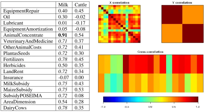
This example is focused on measuring efficiency when the number of DMUs is few and the number of explanatory variables needed to compute the measure of efficiency is too large. We approach this problem through variable aggregation using Canonical correlation analysis. Two preliminary steps calculate the sample correlation coefficients and create a visualization of the correlation matrixes. All sample correlation coefficients are presented in Table 1 and the correlation matrixes are visualized in Figure 1.
In the Table 1 a significant correlation between Milk and AnimalConcentrate is highlighted and we can also note that are nearly null correlation between Milk and Lubricant, Milk and EquipmentAmortization, and Milk and Insurance.
Table 1: Sample correlation coefficients
Figure 1: Plot of correlation coefficients.
Milk Cattle EquipmentRepair 0.40 0.45 Oil 0.30 -0.02 Lubricant 0.01 -0.17 EquipmentAmortization 0.05 -0.08 AnimalConcentrate 0.91 0.54 VeterinaryAndMedicine 0.71 0.37 OtherAnimalCosts 0.72 0.41 PlantasSeeds 0.72 0.30 Fertilizers 0.78 0.45 Herbicides 0.50 0.35 LandRent 0.72 0.34 Insurance -0.07 0.00 MilkSubsidy 0.75 0.43 MaizeSubsidy 0.75 0.53 SubsidyPOSEIMA 0.72 0.08 AreaDimension 0.54 0.28 DairyCows 0.78 0.35
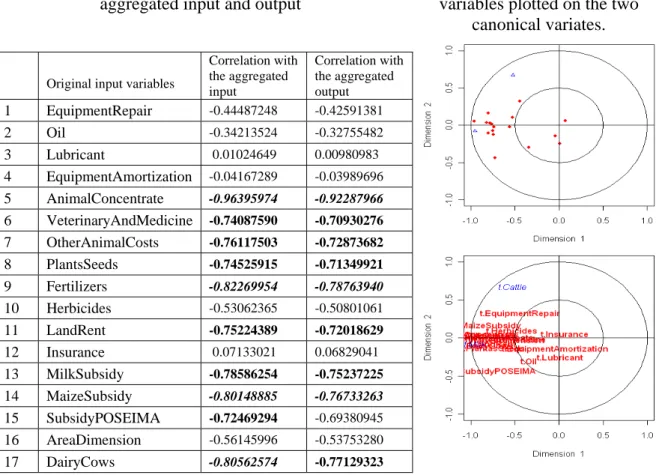
On Figure 2 the input and output variables are plotted on the first two canonical variates. Variables with a strong relation are projected in the same direction from the origin. The greater the distance from the origin, the stronger the relation is. The following variables: AnimalConcentrate, VeterinaryAndMedicine, OtherAnimalCosts, MilkSubsidy, MaizeSubsidy, Herbicides, Fertilizers, PlantsSeeds, LandRent, AreaDimension, DairyCows and Milk are a set of variables with a stronger relation than the rest. In this set AnimalConcentrate, DairyCows, VeterinaryAndMedicine, OtherAnimalCosts and MilkSubsidy are the variables with the strongest relation. MaizeSubsidy and Herbicides are also variables with a strong relation.
Finally, the correlation coeficients between extracted aggregates and original variables are presented in Table 2. In this table values in italic are the highest correlations, as is the case of the correlation between Milk and AnimalConcentrate. We can also see an almost null correlation between Milk and Lubricant, Milk and EquipmentAmortization, and Milk and Insurance. This is almost the same result presented in Table 1, but not quite.
The canonical weights explain the unique contributions of original variables to the canonical variable. Because of existing multicollinearity some canonical coefficients even have a different sign compared to the correlation of the original variable with the canonical variable. Therefore, we follow the standard approach to interpreting the relations of the original variables to a canonical variable in terms of the correlations of the original variables with the canonical variates - that is, by structure coefficients. From Table 2 we can conclude that both canonical variates are predominantly associated with the following original inputs: Animal Concentrate, Fertilizers, DairyCows, MaizeSubsidy, MilkSubsidy, OtherAnimalCosts, PlantsSeeds, LandRent, VeterinaryAndMedicine, SubsidyPOSEIMA and with the original output variable Milk.
Table 2: Correlations of the original inputs with both
aggregated input and output
Figure 2: The input and output
variables plotted on the two
canonical variates.
Original input variables
Correlation with the aggregated input Correlation with the aggregated output 1 EquipmentRepair -0.44487248 -0.42591381 2 Oil -0.34213524 -0.32755482 3 Lubricant 0.01024649 0.00980983 4 EquipmentAmortization -0.04167289 -0.03989696 5 AnimalConcentrate -0.96395974 -0.92287966 6 VeterinaryAndMedicine -0.74087590 -0.70930276 7 OtherAnimalCosts -0.76117503 -0.72873682 8 PlantsSeeds -0.74525915 -0.71349921 9 Fertilizers -0.82269954 -0.78763940 10 Herbicides -0.53062365 -0.50801061 11 LandRent -0.75224389 -0.72018629 12 Insurance 0.07133021 0.06829041 13 MilkSubsidy -0.78586254 -0.75237225 14 MaizeSubsidy -0.80148885 -0.76733263 15 SubsidyPOSEIMA -0.72469294 -0.69380945 16 AreaDimension -0.56145996 -0.53753280 17 DairyCows -0.80562574 -0.77129323
Then we use aggregated input and output in DEA formulation. As we mentioned above the dairy policy in Azorean Islands depends on Common Agricultural Policy of the European Union and it is limited by quotas. Because of it we apply an input oriented DEA model on aggregated measures. On Figure 3 all DMUs and the efficient frontier are plotted.
Figure 3: Results for the BCC Model using
agregated input and agregated output.
5 Conclusions
The proposed methodology, using CCA, provides an aggregation of both input and output variables and then DEA provides efficient units. The aggregation is very useful for small data sets as it is possible to include results for many inputs and outputs without the problems known as “curse of dimensionality”. If we extract only two we also can plot very clear efficiency frontier graphs as the one presented in Figure 3, where we can see that farms 3, 8, 14, 17 and 20 are full efficient, and farms 30 and 12 are the most inefficient. This corroborated by domain knowledge as some of this farms were very well classified in other studies using older data (see Silva, et al., 2004).
In spite of this inspiring result much more work is needed to validate variable aggregation by the approach proposed, and this will be a question for our future research.
We still don’t show, in this work, any results for variable selection. We intend to explore the possibility of using coefficients in table 2 or similar to select variables appropriate for DEA and efficiency measures. This approach should be much simpler than any stepwise or “leave one out” method.
Acknowledgments
This work has been partially supported by Direcção Regional da Ciência e Tecnologia of Azores Government through the project M.2.1.2/l/009/2008.
6 References
Cazals, C.; Florens, J.P. e Simar, L. (2002). Non parametric frontier estimation: A robust approach. Journal of Econometrics, Vol 106, pp. 1-25.
Chilingerian J.A. (1995). Evaluating physician efficiency in hospitals: A multivariate analysis of best practices. European Journal of Operational Research, Vol 80, pp. 548-574.
Cinca, C. Serrano and Molinero, C. Mar (2004). Selecting DEA specifications and ranking units via PCA. Journal of the Operational Research Society, Vol 55, pp. 521-528.
Cooper, William W.; Seiford, Lawrence M. and Tone, Kaoru (2007). Data Envelopment Analysis: A comprehensive text with models, applications, references and DEA-solver software, Springer, New York, USA. ISBN: 978-0-387-45281-4.
Jenkins, L. and Anderson, M. (2003). A multivariate statistical approach to reducing the number of variables in data envelopment analysis. European Journal of Operational Research, Vol 147, pp. 51-61.
Levine, Mark S. (1977) Canonical analysis and factor comparison, Sage Publications, Thousand Oaks, USA. Quantitative Applications in the Social Sciences Series, No. 6. Lewin, A.Y.; Morey, R.C. and Cook, T.J. (1982)0. Evaluating the administrative efficiency of courts. Omega - International Journal of Management Science, Vol 10, No 4, pp. 401-411. Norman, M. and Stoker, B. (1991). Data Envelopment Analysis - The assessment of performance, John Wiley & Sons. ISBN: 0471928356.
Nunamaker, Thomas R. (1985). Using data envelopment analysis to measure the efficiency of non-profit organizations: A critical evaluation. Managerial & Decision Economics, Vol 6, No 1, pp. 50-58.
Salinas-Jiménez, Javier and Smith, Peter (1996). Data envelopment analysis applied to quality in primary health care. Annals of Operations Research, Vol 67, No 1 Sep, pp. 141-161.
Silva, Emiliana; Arzubi, Amílcar e Berbel, Julio (2004). An application of data envelopment analysis (DEA) in Azores dairy farms, Portugal. New MEDIT. A Mediterranean Journal of Economics, Agriculture and Environment, Vol 3, No 3, pp. 39-43.
Sigala, M.; Airey, D.; Jones, P. and Lockwood, A. (2004). ICT paradox lost? A stepwise DEA methodology to evaluate technology investments in tourism settings. Journal of Travel Research, Vol 43, pp. 180-192.
Wilson, Paul W. (1993). Detecting outliers in deterministic nonparametric frontier models with multiple outputs. Journal of Business & Economic Statistics, Vol 11, pp. 319-323.