ABSTRACT: This paper introduces a new approach to represent the rocket exhaust efluents into an atmospheric dispersion model considering the trajectory and variable burning rates of a Satellite Vehicle Launcher, taking into account the buoyancy of the exhausted gases. It presents a simulation for a Satellite Vehicle Launcher light at 12:00Z in a typical day of the dry season (Sept 17, 2008) at the Centro de Lançamento de Alcântara using the Weather Research and Forecasting Model coupled with a modiied chemistry module to take into account the gases HCl, CO, CO2, and particulate matter emitted from the rocket engine. The results show that the HCl levels are dangerous in the irst hour after the launching into the Launch Preparation Area and at the Technical Meteorological Center region; the CO levels are critical for the irst 10 min after the launching, representing a high risk for human activities at the proximities of the launching pad.
KEYWORDS: Satellite Vehicle Launcher, Mesoscale model, Atmospheric dispersion model, HCl.
The Use of an Atmospheric Model to
Simulate the Rocket Exhaust Efluents
Transport and Dispersion for the Centro
de Lançamento de Alcântara
Daniel Schuch1, Gilberto Fisch2
INTRODUCTION
he Centro de Lançamento de Alcântara (CLA) is the Brazilian access to the space, located at the north part of the northeastern region of Brazil. It has some advantages due to its geographical position close to the Equator, which allows rocket launchings that consume less propellant for geostationary satellite missions. Other advantages are associated with its proximity of São Luís (capital of Maranhão State) as well as its low population density, so the health risks of contamination by gases sent out from launchings are reduced. Rockets such as the Veículo Lançador de Satélites (VLS) are launched from this Range Center.
During the irst few seconds following the ignition of the engine, the VLS releases a large cloud of hot, buoyant exhaust products near the ground level which rise and entrain into atmosphere until reach an approximate equilibrium with the ambient conditions. his cloud is composed by the products of the combustion of perchlorate and aluminum: hydrogen chloride (HCl), water (H2O), carbon monoxide (CO), carbon dioxide (CO2), and particulate material composed by aluminum oxide (Al2O3) used into the grain composition of the solid propellant (Denison et al. 1994).
All the Space Centers around the world have adopted some models in order to predict these gases dispersions. For instance, the East US Space Ranger Center (like NASA JFK/U. S. Cape Canaveral) uses an operational model known as Rocket Exhaust Eluent Difusion Model (REEDM) and it has been used to assess the environmental impact of aerospace activities (Bjorklund
1.Departamento de Ciência e Tecnologia Aeroespacial – Instituto Tecnológico de Aeronáutica – Programa de Pós-Graduação em Ciências e Tecnologias Espaciais – São José dos Campos/SP – Brazil. 2.Departamento de Ciência e Tecnologia Aeroespacial – Instituto de Aeronáutica e Espaço – Divisão de Ciências Atmosféricas – São José dos Campos/SP – Brazil.
Author for correspondence: Daniel Schuch | Departamento de Ciência e Tecnologia Aeroespacial – Instituto Tecnológico de Aeronáutica – Programa de Pós-Graduação em Ciências e Tecnologias Espaciais | Praça Marechal Eduardo Gomes, 50 – Vila das Acácias | CEP: 12.228-901 – São José dos Campos/SP – Brazil | Email: [email protected]
et al. 1982). his dispersion model is based on Gaussian model concepts: the exhaust material (mixture amongst CO, CO2, HCl, and Al2O3) is assumed to be uniformly and vertically distributed and to have a bivariate Gaussian distribution in the plane of the horizon at the point of cloud stabilization, which is determined by the cloud rise theory.
The model used at the European Spaceport of Kourou (French Guyana) is the SARRIM Software (Cencetti et al. 2011), which considers the emissions divided into “pufs” from the launching pad up to the stabilization height, dealing with the local and large scale impact assessment for propellant and hypergolic rocket releases. It is an operational and fast running tool taking into account atmospheric thermal stratiications inside the boundary layer using in situ data like radiosondes.
he India Space Center (Satish Dhawan Space Center SDCS SHAR) has coupled a Hybrid Single-Particle Lagrangian Integrated Trajectory (HYSPLIT) model with an atmospheric mesoscale one (in this case, it was used the mesoscale meteorological model-MM5) to predict the dispersion of exhaust pollutant in the form of vapor and ground level concentrations (Rajasekhar et al. 2011).
he Brazilian community is also addressing this problem for CLA since 2010 and it was developed the Modelo Simulador da Dispersão de Eluentes de Foguetes (MSDEF), which represents the solution for time-dependent advection-difusion equation applying the Laplace transform considering the Atmospheric Boundary Layer as a multilayer system. his solution allows a time evolution description of the concentration ield emitted from a source during a release lasting time; it takes into account deposition velocity, first-order chemical reaction (decay), gravitational settling, precipitation scavenging, and plume rise efect. A detail description of this model can be found in Moreira et al. (2011). In Nascimento et al. (2014), the authors coupled this model to the Weather Research and Forecasting Model (WRF), for the meteorological forecast, and to the Community Multi-scale Air Quality model (CMAQ), for the chemistry. Moreover, Iriart and Fisch (2016) used the WRF coupled with this chemistry module (Chem). Both studies addressed the CLA dispersion problem for air quality models.
In this study we propose a new representation of a rocket emission, taking into account the plume rise efect, trajectory, and variable emissions rates (in time and space), into a meteorological/ chemical model in order to achieve a better vertical distribution of the emissions and then predict the transport, dispersion, and atmospheric reaction of the gas exhausted. A simulation using data of the Brazilian VLS was assessed using the WRF
model (version 3.7.1) with a modiied Regional Atmospheric Chemistry Mechanism (which includes HCl) for the CLA region.
METHODOLOGY
he WRF model is a numerical weather prediction system, considered the state-of-the-art, designed for both atmospheric research and operational forecasting needs, being applied to a wide range of meteorological problems with scales from tens of meters to thousands of kilometers. he coupling of the meteorology and chemistry (into the WRF-Chem coupled) is calculated on-line (without loss of information), and the meteorological process of transport, radiation, and reactions is fully coupled (interacting with each other) and solved simultaneously without any type of interpolation (Grell et al. 2005; Skamarock et al. 2008).
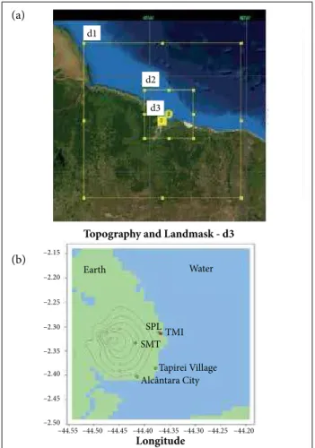
For the simulations, 3 nested domains centered into the Setor de Preparação de Lançamento (SPL), where the rocket is launched, were chosen. he outer domain (d1) is a 100 × 100 grid points with 9 km of horizontal resolution; the middle domain (d2) has 70 × 70 points and 3 km of resolution; the inner domain (d3) has 40 × 40 points with 1 km of horizontal resolution. All domains have 43 vertical levels, from surface up to 30 km, distributed mainly close to the surface. Figure 1a shows an image of the region and the 3 domains.
he static data (topography, land mask, vegetation, etc.) used was provided by the United States Geological Survey (available from: http://www.mmm.ucar.edu/wrf/src/WPS_files/geog. tar.gz) with spatial resolution of 30” (this data is usually used to weather forecasts). Figure 1b shows the topography (lines) and landmask (colors) for the inner domain (d3). Also, it was marked the position of some buildings that are part of the CLA’s structure: SPL and the Setor de Meteorologia (SMT), as well as the only habited areas nearby: the city of Alcântara (CLA) and the Tapireí village (VTA).
For the WRF coniguration, it was used the following set of parametrizations:
• Microphysics: WRF Single-Moment 3-class Scheme, simple and eicient scheme which contains ice process adapted to large scale.
• Long wave radiation: Rapid Radiative Transfer Model (RRTM), a scheme which utilizes tables of radiation eiciency.
• Short wave radiation: Dudhia scheme, simple scheme of integration which allows the absorption of radiation in clear sky from the clouds and scattering by atmosphere. • Supericial layer: MYNN surface layer, Nakanishi and
Niimo scheme.
• Surface: Noah Land Surface Model, scheme of soil temperature and humidity with 4 layers.
• Planetary Boundary Layer (PBL): Mellor Yamada Nakanishi and Nimo level 2.5, scheme with prediction of turbulent kinetic energy to the model sub-grid.
• Cumulus: Grell 3D, enhanced scheme of Grell-Devenyi which can be used for high spatial resolutions (turned of in the d3 domain).
Due to the necessity of representing all the emitted species by the combustion of the rocket solid propellant into the WRF model, especially the species HCl, a new chemistry mechanism based on the RACM (Stockwell et al. 1997) was created. HCl and more 5 chlorinated species were added (Cl, Cl2, HOCl, ClO, and formyl luoride), as well as 3 photoreactions, 5 inorganic reactions, and 11 organic reactions from the CB05 mechanism (Yarwood et al. 2005) inside the RACM.
Since version 2.2, the WRF model was released with the kinetic preprocessor (KPP) built in the source code. It was designed as a general analysis tool to facilitate the numerical solution of chemical reaction network problems. he KPP subroutines automatically generate FORTRAN code that computes the time-evolution of chemical species, starting with a speciication of the chemical mechanism. KPP further allows a rich selection of numerical integration schemes and provides a framework for evaluation of new integrators and chemical mechanisms (Damian et al. 2002).
he interaction of the KPP and WRF is made by a subprogram named WRF-KPP-Coupler (WKC). Once the KPP option is enabled, the WRF’s compilation script compiles and executes the WKC, and the KPP generates all the code to compile WRF, including the new mechanism. Even though the WKC generates the code to be integrated into the model, the mechanism needs to be included to the ile Registry.chem in order to be recognized by the model. Consequently, the Chem module must be modiied in order to include the new mechanism in the processes of initialization, calculation of velocities of deposition, diferent emission options, and optical proprieties.
REPRESENTATION OF SATELLITE
VEHICLE LAUNCHER EMISSIONS
In air quality (AQ) models, the way emissions are represented is the most critical input parameter and has greater impact into the inal concentration of the contaminant. he inclusion of a source like the VLS into WRF needs some considerations: the rocket like the fuel expenditure, vertical trajectory, and the type of propellant used should be taken into account as well as the limitations of the model for time and space scales.
Figure 1. (a) Domains of simulation; (b) Topography (lines) and landmask (green for continent and blue for water) of inner domain.
Topography and Landmask - d3
Longitude TMI SPL SMT
Alcântara City Tapirei Village
Water Earth
d1
d2 d3
–2.15
–2.20
–2.25
–2.30
–2.35
–2.40
–2.45
–2.50
–44.55–44.50–44.45–44.40 –44.35–44.30–44.25 –44.20
(a)
he total mass of gases released into atmosphere in a VLS launch is given by:
H is the Heaviside function (whose value is 0 for negative and 1 for positive argument); zm is the height of the top of the layer m; zm−1 is the top of the layer below the surface (z0); ∂M/∂t is function of height and time.
For VLS emission scenarios, the exhaust from the rocket combustion is at several thousand Kelvin degrees and highly buoyant. he high temperature of these exhaust emissions causes the plume to be less dense than the surrounding atmosphere, and buoyancy forces acting on the cloud can cause it to lit of the ground and accelerate vertically. As the buoyant cloud rises, it entrains ambient air and grows in size while also cooling. In this initial cloud rise phase, the growth of the cloud volume is due primarily to internal velocity gradients and mixing induced by large temperature gradients within the cloud itself. Even though the cloud is entraining air and cooling due to the mixing hot combustion gases with cooler ambient air, the net thermal buoyancy in the cloud is conserved, and the cloud will continue to rise until it either reaches a stable layer in the atmosphere or the cloud vertical velocity becomes slow enough to be damped by viscous forces (Nyman 2009).
Considering that the WRF model does not have a general scheme for plume rise, we have assumed that the plume is released into a height matching the rocket trajectory plus a plume rise (Δz) height. For the determination of this height rise, the following parametrizations were adopted, in which the height is calculated directly by a model based on Briggs (1975). For an instantaneous cloud rise scheme, this rise is deined as where: ∂M/∂tis the fuel expenditure rate (g/s), which varies
with time along the trajectory of the rocket; t0 is the ignite time; and tN is the time when the fuel is completely burned.
As the shortest interval for data input of WRF is 1 min, the emissions were split in min by min as
(1)
(2)
where: tn = 60n (s), and each term represents an emission ile for the model.
For the vertical domain, the WRF model was discretized into sigma levels, which is a normalized coordinate (assuming unitary value at surface and 0 on the top of the domain) following the topography (Fig. 2).
Figure 2. Layers and the rocket trajectory.
σ
0= 1.0
σ
1σ
2σ
Mσ
Mσ
M=0
z
0= 0.0
z
1z
2z
M–2z
M–1z
MWhereas the rocket it is not a ixed source, the distribution of emission should follow the rocket trajectory and is allocated into M model layers as follows:
(3)
(5)
(6) (4)
where:
where: Fi= buoyancy term = 3gq/4πρCρTa; Ta(m4s2) is the ambient temperature (K);
ρ
is the air density (kg/m3); Cp is the speciic heat of exhaust cloud gases = 1.7755 (cal/kgK);
q = initial heat of the plume = H (∂M/∂t) бt (cal); H is the efective fuel heat content (cal/g); γ is the air entrainment coei- cient = 0.64 (dimensionless); s = atmosferic stability parameter
g/θ0(Δθ0/Δz)(s–1); g is the gravitational acceleration cons- tant = 9.81 (m/s2); θ
0 = potencial temperature of ambient air = Ta(p0/p)R/Cp (K).
where: ti is constrained to be less than the cloud stabilization time: increment to be used is the smallest between Δzi, Δzc, and Δzn. his suggestion is the most prudent due to the fact that, as the rise efect is larger, the concentration values obtained at surface level are smaller, reducing the risk of underestimating the value of these concentrations.
Once the plume rise height is calculated, the emission into the WRF model can be written as
he height of the rise in a continuous plume in a stable atmosphere is deined as
(7)
(8)
(9)
(11)
(12)
(10) where: Fc = buoyancy term = gq/πρCρTa(m4s2) ; γ is the air entrainment coeicient = 0.5 (dimensionless).
And the time for a continuous plume to reach the height
zkin a stable atmosphere is given by
where: tc is constrained to be less than t*, described by Eq. 7, and u is the wind velocity (Bjorklund et al. 1982).
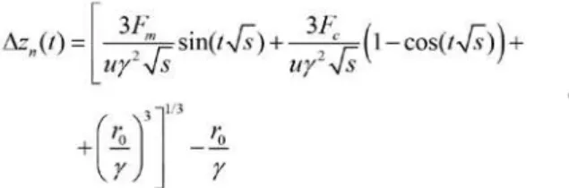
The following equation was based on a solution of the Newton’s second law and solved iteratively to predict the motion of a buoyant cloud in the atmosphere, resulting in cloud stabilization height:
where: Fm is the initial vertical momentum = r0w0u (m4s2); r 0is the initial plume cross-sectional radius = 3.5 (m); w0 is the initial vertical velocity (m/s); u is the mean ambient wind speed (m/s);
γ is the air entrainment coeicient = 0.33 (dimensionless); ρ is the density of exhaust gases = 0.109 (kg/m3).
A critical parameter in the cloud rise equation is the rate of ambient air entrainment that is deined by γ. Cloud growth as a function of altitude is assumed to be linearly proportional, and the air entrainment coeicient have been compared from the literature (observations and measurements of Titan IV rocket ground clouds), and an empirical cloud rise air entrainment coeicient has been derived from the test data (Nyman 2009). It should be noticed that there is no data of this nature for VLS.
Considering the diferent formulations from Eqs. 5 to 10, Briggs (1975) suggests that the value of the rise height
when i = iTMI and j = jTMI or
where: i ≠ iTMIor j ≠ iTMI. he indexes i and j are horizontal grid coordinates of the model.
he rocket is launched from the point (iTMI, jTMI) of the WRF inner domain of simulation (d3). Note that Eqs. 11 and 12 disregard the horizontal component of the rocket displacement, but it is a ine assumption even into the inest scale models.
Table 1 shows the composition of the exhaust gases of the VLS, the mass percentage gas, and the variable into WRF. HCl, CO, and CO2 are pollutants into gaseous form, and Al2O3 is divided into 2 sizes of particulate matter of 2.5 mm (pm 2.5) and 10 mm (pm 10).
Species % Variable
Alumina Al2O3 28.4 pm 2.5 + pm 10
Carbon monoxide CO 28.7 CO
Hydrogen chloride HCl 21.4 HCl
Nitrogen N2 8.3
-Water vapor H2O 6.8
-Carbon dioxide CO2 3.6 CO2
Hydrogen H2 2.8
-Table 1. Composition of the exhaust gases of VLS.
RESULTS AND DISCUSSION
For the simulations, we have chosen a typical clear sky day from the dry season (Sept 17, 2008), where the model started at 00:00Z and the release of VLS gases occurred at 12:00Z, considering 12 h for the model spin-up. With a radiosonde released at 11:32Z, the mean wind within the planetary boundary layer (about 600 m) is about 13 m/s and the atmospheric stability is unstable, favoring the turbulence. hese are characteristics of a suitable day for a rocket launching (wind speed below 10 m/s at surface level, lower wind speed up to 5 km, no rain, etc.) and good conditions for dispersion (presence of an atmosphere unstable) and transport (strong influences of the trade winds) of the rocket eluents.
Figure 3 shows the vertical distribution of the VLS emissions using Eq. 12 for the VLS data and the distribution used by Nascimento et al. (2014) for a hypothetical launching of a Titan-IV rocket. It can be observed that the distribution of emissions for the VLS is quite diferent from Titan-IV: it is lower close to the surface and higher at 1 – 2 km.
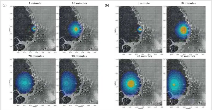
Figure 4 shows a time sequence of arrow plots of the horizontal component of the wind at the surface level, whose direction is predominantly from east. The wind speed is above 7 m/s in the ocean region and becomes weaker
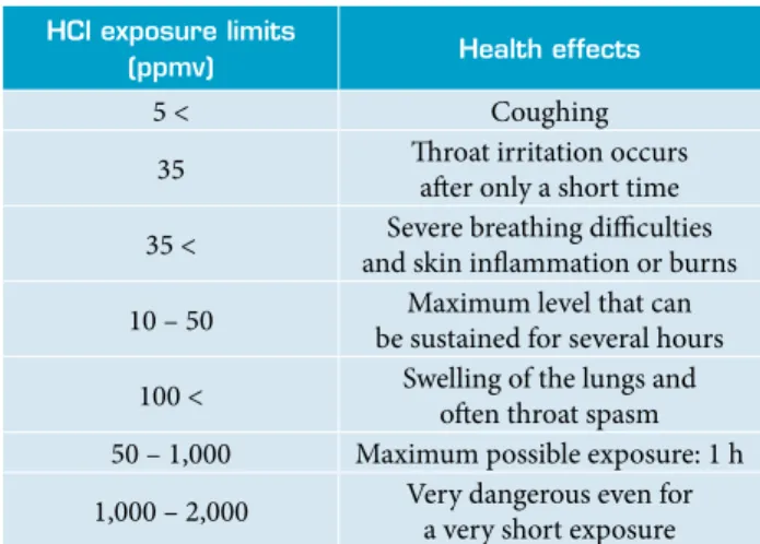
inland the continent (about 6 m/s in the SPL). The shaded areas represent the HCl concentration at the first layer of the model (approximately 40 m) for the initial 30 min after the launching of VLS. These plots have a log scale for the concentration for a better visualization. In this figure we can observe the exhausted cloud behaviors after the rocket launching: initially it presents a maximum concentration at the launch pad (SPL and TMI) and it is advected and dispersed with time. This plume reached the SMT with a still higher concentration (around 176 ppmv) within about 10 min. The other locations (CLA and VTA) were not reached by this plume. HCl is a colorless gas with an irritating pungent odor perceivable at 0.8 ppmv (Lide 2003). Table 2 presents the hydrogen chloride exposure limits (Braxter et al. 2000).
Figure 3. Emissions for the VLS and Titan-IV.
H
eig
h
t [k
m]
3.0
2.5
Nascimento et al. 2014 Present work
2.0
1.5
1.0
0.5
0.0
0 5 10 15 20 25 30
Distribution of the VLS-01 emissions
Weight [%]
HCl exposure limits
(ppmv) Health effects
5 < Coughing
35 hroat irritation occurs
ater only a short time
35 < Severe breathing diiculties and skin inlammation or burns
10 – 50 Maximum level that can be sustained for several hours
100 < Swelling of the lungs and oten throat spasm 50 – 1,000 Maximum possible exposure: 1 h
1,000 – 2,000 Very dangerous even for a very short exposure Table 2. Health effects of respiratory exposure to HCl concentration.
Figure 4b presents the same information of Fig. 4a for CO concentrations and it is diferent from Iriart and Fisch (2016) by 2 reasons: the amount of gases exhausted is associated with a real value for VLS launching and this material is released during the lights trajectory (vertical dependence). For this variable we can notice the larger areas with higher concentrations that persist beyond the plume passage. However, this variable is not so toxic as HCl.he CO is a colorless and odorless gas that is slightly less dense than air. It is toxic to humans (and another hemoglobic animals) when observed in concentrations above about 35 ppmv. In the atmosphere, it is spatially variable and short-lived, having a role in the formation of ground-level ozone. he recommendation of the World Health Organization (1999) is that the exposure times should not exceed those shown in Table 3.
1 minute 10 minutes
20 minutes 30 minutes
1 minute 10 minutes
20 minutes 30 minutes
Figure 4. Surface concentrations after launching of (a) HCl and (b) CO.
(a) (b)
Figure 5a shows a time series of the HCl concentrations (presented in a logarithm scale) for up to 2 h after the launching for the locations SPL, SMT, CLA, and VTA. The higher levels are between 1,540 ppmv (SPL) and 176 ppmv (SMT) and, according to Table 2, the maximum exposure time is only 1 h; the inhalation of the gas can cause swelling of the lungs, throat spasm, and irritation. In the surrounding area, it presents concentration levels between 0.11 ppmv (VTA) and 0.53 ppmv (CLA), which are safety values of HCl, with effects imperceptible to the majority of the population.
Figure 5b presents the CO concentrations in function of time. The higher levels are in the range between 2,735 ppmv at SPL and 176 ppmv at SMT. From Table 2, a maximum exposure time is between 30 min and 2 h, and this may cause headache, increased heart rate, dizziness, nausea, and even
CO exposure limits (ppmv) Maximum exposition time
9 8 h
26 1 h
52 30 min
87 15 min
1,950 Rapidly fatal
Table 3.Exposure limits for CO.
Source: extracted from Winter and Miller (1976).
death. In the surrounding area, it presents concentration levels below 2 ppmv (CLA and VTA), which are safety for the mankind.
Figure 5c shows the concentration of the CO2 with a peak of 598 ppmv at SPL. It is considered the minimal value for an effect on health by CO2 inhalation of 15,000 ppmv during 1 month of exposure. In practical sense these values of CO2 concentration have no effect for the humans.
Figure 6 shows the particulate material with 10- and 2.5-mm concentrations composed by Al2O3 in function of time. he levels for the CLA and the VTA are below 1 mg/m3.
The World Health Organization (2000) guidelines do not recommend the use of levels of pm 10 and pm 2.5 as long as there are no suicient data to enable the derivation of speciic values at present. Nevertheless, the large body of information on studies relating day-to-day variations in particulate matter to day-to-day variations in health provides quantitative estimates of the efects of particulate matter that are generally consistent. he available information does not allow a judgment to be made on concentrations below, in which no efects would be expected.
CONCLUSION REMARKS
In this paper we present a way to include the major atmospheric pollutants emissions from the VLS into a weather model (WRF-Chem) taking into account the vertical distribution of emission and the efect of buoyancy of the hot cloud formed by the eluents. his implementation represents an improvement to the study of Iriart and Fisch (2016), in which the emissions were made only at the surface level (without accounting the efect of buoyancy, trajectory, and variable emissions rates), not considering HCl; this features allowed us to use data from the Brazilian rocket VLS (instead of Titan-IV data) and analyze more realistic concentrations at the closer sites of the VLS launcher pad as the plume behavior for the CLA region.
he results show that the HCl levels are dangerous in the irst hour ater the launching at the SPL and SMT regions; the CO levels are more critical for the irst 10 min ater the launching, representing a high risk at the proximities of the SPL and attention state on the SMT. he concentrations of CO2, pm 2.5, and pm 10 showed secure levels even for the proximities 420 mg/m3, and emergency for values beyond 500 mg/m3.
These values are for both pm 10 and pm 2.5, being calculated as an average during a time interval over 24 h. The maximum values for the pm 10 and pm 2.5 are 30.3 and 273.5 mg/m3, respectively. The peak concentration of pm 10 is below the regular level adopted (50 mg/m3), considered a secondary air quality standard or, in other words, a level in which it provides the minimum adverse effect on human health. However, the pm 2.5 concentration peaks are next to the attention level, but the mean value for the first hour is approximately 14 mg/m3.
Figure 5. Time series of simulated and the levels of health effects for (a) HCl; (b) CO and (c) CO2.
10 00 100 200 500 1,000 2,000 5,000 30
20 40 50 60 70
Minutes
8090100110120 10
00 20 3040 50 60 70
Minutes
8090100110120 10
00 20 3040 50 60 70
Minutes
8090100110120
0.1 0,5 2 50 200 2,000 500 5 10 20 1e-C4 0.001 5,000 500 100 20 5 0.01 0.1 0.5
5,000-10,000 ppmv - no detectable limitations
380 ppmv - typical atmospheric value 9 ppmv - 8h 26 ppmv - 1h 52 ppmv - 30 min 87 ppmv - 15 min
1950 ppmv - Rapidly fatal 5 ppmv - coughing
35 ppmv - few hours 100 ppmv - max 1 hour 1,000 ppmv - short period
50 ppmv - max 1 hour
SPL SMT ALC VTA CO 2 [p p m v] C O [p p m v] H CL [p p m v] 10
00 20 3040 50 60 70
Minutes
PM 2.5μ (μ/kg dr
y a
ir)
PM 10μ (μ/kg dr
y a
ir)
80 90100110120 10
00 20 3040 50 60 70
Minutes
8090 100110120
0.1 0.2 0.5 5 10 50 7 20 1 2 1 2 500 200 100 50 4 10 20
regular - 50μg/kg dry air
regular - 60μg/kg dry air
inappropriate - 150μg/kg dry air bad - 250μg/kg dry air health risk - 420μg/kg dry air Particulate matter - 10μ
SPL SMT
Figure 6. Time series of simulated and the levels of health effects for (a) pm 10 and (b) pm 2.5.
(a) (a)
(b) (b)
of the SPL; inally, the exhaust cloud does not reached the CLA or the VTA, mainly due to the wind direction.
After 40 min of the VLS launching the clouds were dispersed and left the inner domain, which is the region of interest. This means that the levels of each pollutant are below the minimum concentration for a detectable effect on the human health.
As the transport and dispersion of the rocket effluents depend tightly on the atmosphere state, the simulations are not a general solution for the problem, but represent a very good prediction scenario. Stronger or weaker winds (or different wind directions) can make the transport more or less efficient (as well as allow the plume to reach different locations), and different stability conditions (stable or unstable) will affect the dispersion by reducing the turbulent mixing, resulting in higher (or lower) concentrations. Other simulations for different atmospheric stability and wind directions will be made for more general assumptions and case studies.
In a future study, we will focus our attention on the chemical mechanism, where the aterburn and HCl atmospheric reactions must be included into the chemical module of WRF for a more
realistic representation of the atmospheric chemical inluence of the eluents of rocket exhausts.
ACKNOWLEDGEMENTS
he authors thank the Coordenação de Aperfeiçoamento de Pessoal de Nível Superior (CAPES), who funded part of this research through the project PRO-ESTRATEGIA (number 2240/2012), as well as provided the scholarship grant PQ (number 308011/2014). At last, but not least, a special thanks to Dr. Stacy Walters, from he University Corporation for Atmospheric Research (UCAR), who contributed for this study with a very important support.
AUTHOR’S CONTRIBUTIONS
Schuch D performed the experiments and prepared the figures. Schuch D and Fisch G discussed the results and commented on the manuscript.
REFERENCES
Bjorklund JR, Dumbauld JK, Cheney CS, Geary HV (1982) User’s manual for the REEDM (Rocket Exhaust Effluent Diffusion Model) computer program. NASA Contractor Report 3646. Huntsville: NASA George C. Marshall Space Flight Center.
Brasil. Ministério do Meio Ambiente (1990) Resolução CONAMA nº 3, de 28 de junho de 1990; [accessed 2017 Jan 19]. http:// www.mma.gov.br/port/conama/legiabre.cfm?codlegi=100
Braxter PJ, Adams PH, Cockcroft A, Harrington JM (2000) Hunter’s diseases of occupations. 9th ed. London: Arnold; New York: Oxford University Press.
Briggs GA (1975) Plume rise predictions. Lectures on Air Pollution and Environmental Impact Analysis. Amer Meteor Soc (72-73):59-111. doi: 10.1007/978-1-935704-23-2_3
Cencetti M, Veilleur V, Albergel A, Olry C (2011) SARRIM: A tool to follow the rocket releases used by the CNES Environment and Safety Division on the European Spaceport of Kourou (French Guyana). Int J Environ Pollut 44(1-4):87-95. doi: 10.1504/IJEP.2011.038406
Damian V, Sandu A, Damian M, Potra F, Carmichael GR (2002) The kinetic preprocessor KPP – a software environment for solving chemical kinetics. Comput Chem Eng 26(11):1567-1579. doi: 10.1016/S0098-1354(02)00128-X
Denison MR, Lamb JJ, Bjorndahl WD, Wong EY, Lohn PD (1994) Solid rocket exhaust in the stratosphere: plume diffusion and chemical reactions. J Spacecraft Rockets 31(3):435-442. doi: 10.2514/3.26457
Emmons LK, Walters S, Hess PG, Lamarque JF, Pfister GG, Fillmore D, Granier C, Guenther A, Kinnison D, Laepple T, Orlando J, Tie X, Tyndall G, Wiedinmyer C, Baughcum SL, Kloster S (2010) Description and evaluation of the Model for Ozone and Related chemical Tracers, version 4 (MOZART-4). Geosci Model Dev 3:43-67. doi: 10.5194/gmd-3-43-2010
Grell GA, Peckham SE, Schmitz R, McKeen SA, Frost G, Skamarock WC, Eder B (2005) Fully coupled “online” chemistry within the WRF model. Atmos Environ 39(37):6957-6975. doi: 10.1016/j. atmosenv.2005.04.027
Iriart PG, Fisch G (2016) Uso do modelo WRF-Chem para a simulação da dispersão de gases no Centro de Lançamento de Alcântara. Rev Bras Meteorol 31(4):610-625. doi: 10.1590/ 0102-7786312314b20150105
Lide DR (2003) CRC handbook of chemistry and physics. 84th ed. Boca Raton: CRC Press.
Moreira DM, Trindade LB, Fisch G, Moraes MR, Dorado RM, Guedes RL (2011) A multilayer model to simulate rocket exhaust clouds. J Aerosp Technol Manag 3(1):41-52. doi: 10.5028/ jatm.2011.03010311
Nyman RL (2009) NASA Report: Evaluation of Taurus II Static Test Firing and Normal Launch Rocket Plume Emissions.
Pfister GG, Parrish DD, Worden H, Emmons EK, Edwards DP, Wiedinmyer C, Diskin GS, Huey G, Oltmans SJ, Thouret V, Weinheimer A, Wisthaler A (2011) Characterizing summertime chemical boundary conditions for airmasses entering the US West Coast. Atmos Chem Phys 11:1769-1790. doi: 10.5194/acp-11-1769-2011
R Core Team (2015) R: A language and environment for statistical computing; [accessed 2016 Apr 28]. https://www.R-project. org/
Rajasekhar M, Kumar MD, Subbananthan T, Srivastava V, Apparao B, Rao VS, Prasad M (2011) Exhaust dispersion analysis from large solid propellant rocket motor firing using HYSPLIT model over Satish Dhawan Space Centre (SDSC SHAR). Proceedings of the Indo-US Conference-cum-Workshop on “Air Quality and Climate Research”; Hyderabad, India.
Skamarock WC, Klemp JB, Dudhia J, Gill DO, Baker DM, Duda MG, Huang XY, Wang W, Powers JG (2008) A description of the
Advanced Research WRF version 3. Technical Note. Boulder: National Center for Atmospheric Research.
Stockwell WR, Kirchner F, Kuhn M, Seefeld S (1997) A new mechanism for regional atmospheric chemistry modeling. J Geophys Res 102(D22):25847-25879. doi: 10.1029/97JD00849
Winter PM, Miller JN (1976) Carbon monoxide poisoning. J Am Med Assoc 236(13):1502-1504. doi: 10.1001/ jama.1976.03270140054029
World Health Organization (2000) Air quality guidelines for Europe. WHO regional publications: European series, n. 91; [accessed 2016 Apr 20]. http://www.euro.who.int/__data/assets/pdf_ file/0005/74732/E71922.pdf
World Health Organization (1999) Environmental Health Criteria 213: carbon monoxide. 2nd ed.; [accessed 2015 Oct 28]. http:// www.who.int/ipcs/publications/ehc/ehc_213/en/