ULTRASOUND VELOCITY PROFILE (UVP) MEASUREMENTS
IN SHALLOW OPEN-CHANNEL FLOWS
João N. Fernandes
1, João B. Leal
2and António H. Cardoso
3 1Department of Hydraulics and Environment, National Laboratory for Civil Engineering (LNEC), Portugal
2CEHIDRO & Department of Civil Engineering, FCT, Universidade Nova de Lisboa, Portugal
3CEHIDRO & Department of Civil Engineering and Architecture, Instituto Superior Técnico, Portugal
email: jnfernandes@lnec.pt
ABSTRACT
This paper is concerned with velocity measurements in shallow water flows by using Ultrasonic Velocity Profile (UVP) probes. The measurements were made in a 10 m long, 0.4 m wide flume whose slope is 0.00117. Diagonal and
horizontal positioning of a single probe and the combination of two probes were tested as configurations of the UVP probes. Streamwise and transverse velocities were obtained. A sensitivity analysis was performed to UVP parameters, namely to the distance of the window for each measurement and to the distance between each measuring point. The influence of four different seeding materials was also assessed. Filters for eliminating noise and spikes were applied. For 1D measurements, UVP streamwise velocities were compared with Pitot tube measurements. For 2D
measurements, streamwise velocities and turbulent intensities were compared with known laws. The results show the importance of i) setting optimal UVP parameters values, ii) of positioning adequately the UVP probes and iii) using appropriate seeding.
INTRODUCTION
The measurement of instantaneous velocities in water flows has long been a challenging issue. Different measuring equipment has been used, ranging from expensive and complex laser Doppler systems to less expensive but still robust equipment like the Pitot tube. Due to their relatively low price and easy handling, Acoustic Doppler systems are widely used at present. Ultrasound (US) systems, based on echography and Doppler effect, allowed the development of equipment capable of measuring almost instantaneous velocity profiles (Takeda, 1995).
Initially the Ultrasonic Velocity Profile (UVP) technique was limited to opaque fluids (e.g. Takeda and Kikura, 2001, Wiklund et al., 2006) and it was typically used to measure across pipe walls in small scale pressure flows (e.g. Takeda 1995, Ozaki et al., 2002, Kikura et al., 2004). The use of UVP in open-channel water flows (e.g. Kantoush etal., 2008) is recent and still rare. Nevertheless, this technique seems promising since it allows measurements in shallow flows, frequently encountered in experimental facilities, and not achievable with, e.g., Acoustic Doppler Velocimeters (ADV). The UVP probes emit a US beam that travels along the axis and after receive the echo from the same beam as reflected in small particles present in the fluid. The UVP system measures the time delay of the echo to reach the probe and the Doppler frequency shift. Knowing the speed of the sound in the fluid, it calculates the distance and the velocity of the particle. A more detailed description of this technique is presented, for example, by Takeda (1995). Frequently the particles present in the water are sufficient for UVP measurements (Metflow, 2002) but most users apply seeding particles in order to improve the quality of measurements (Wiklund et al., 2006, Kantoush et al., 2008).
An illustration of a US beam, and a graphic scale for a UVP probe with a working frequency of 4 MHz are presented in Figure 1. In the same figure, the main parameters and characteristics of the UVP probes are listed. Each sampling volume represented along the US beam is known as “channel”. In US measurements, the size of the control volume is important (cf. Kikura et al., 2004) but not always easy to identify. As shown in Figure 1, the US beam begins with a diameter equal to the probe diameter (5 mm in the case of the probes used in this study), decreasing in the first part of the path until it reaches the focus point (in water, at 16.9 mm from the probe) where the diameter is 1.35 mm. Then the beam is divergent (2.2º for 4 MHz probes in water). The sampling volume is a cone with planar bases, whose diameters are defined by the beam divergence and the distance from the probe. The thickness (channel width) is defined by the user. This means that velocity consists of the average velocity of the particles in that volume. The highest intensity of the US beam is in its axis, where most of the particles are sampled.
Although the UVP technique has been developed for 1D measurements, measurement of 2D velocity fields using UVP probes has been reported to give promising results (Takeda, 1995, Takeda and Kikura, 2002, Kikura et al., 2004, Kantoush et al., 2008).
Figure 1. Schematic representation of the UVP probe and US beam (parameters 1 to 7 are chosen by the user).
EXPERIMENTAL SETUP, MEASUREMENT EQUIPMENT AND SEEDING
The experiments were made in a 10 m long, 0.4 m wide and 0.1 m high trapezoidal flume with 45º inclined banks. The channel slope is 1.17x10⁻³ m/m and its bottom is made of polished concrete (n = 0.009 m–1/3s). The supply is assured by a constant level reservoir; an electromagnetic flowmeter is used to monitor the flow rate (accuracy of 0.3%). A
honeycomb device and a polystyrene plate were placed at the upstream section of the channel to ensure the flow uniformity and stability. The experiments were done for subcritical flow regime, the water surface level being controlled by a tailgate located downstream. Water depths were measured by using three point gauges.
In all tests, a uniform regime was established corresponding to a water depth equal to 0.06 m and a discharge equal to 13.9 l/s (Reynolds number, Re = 8.56 × 10⁴ and Froude number, Fr = 0.67). The measurements were obtained in a cross section that is 6 m far from the upstream section, to allow for the complete development of the boundary layer.
The velocities were measured using 4 MHz UVP probes and a Pitot tube with 3.2 mm of diameter, connected to a differential pressure transducer. Three different probe set-ups were tested. First, the complete vertical profile of the time averaged velocity was measured by mounting the probe with an angle θ equal to 20º with the flume bottom (Figure 2a).
Secondly, the probe was mounted horizontally, pointing upstream (see Figure 2b, angle θ equal to 90º). This position,
used for instance by Manes et al. (2006), allows the US beam to find more particles and reduce the reflections with an important improvement of the results. Nevertheless it has the disadvantage of taking a profile of the velocity parallel to the bottom. For this configuration, two aspects have been analysed: the UVP system parameters; the influence of seeding conditions. Finally, 2D velocity measurements were made in the centre of the flume with the probes configuration presented in the Figure 2c, allowing the evaluation of the accuracy of time averaged velocities and turbulence intensities measurements.
Figure 2. (a) Diagonal position of the probe; (b) horizontal position of the probe; (c) 2D velocity measurements.
Since the UVP system measures echoes from reflecting particles suspended in the fluid, it is frequently needed to add such particles (seeding). Three types of seeding particles were chosen from the available materials. They consist of crushed nut shell, bakelite and silica powder (Table 1). According to the theory of the US reflection in particles, these particles should have specific density close to 1 and diameter larger than one fourth of the wavelength of the emitted US burst (i.e. particles should have 93 m for 4MHz probes, Metflow, 2002). However, some authors obtained good results using seeding particles with diameters between 3 m and 30 m (e.g. Sato et al., 2002).
Table 1. Seeding particles characteristics.
Materials Specific
gravity
Mean diameter ( m)
Crushed nut shell 0.94 110
Bakelite 1.25 40
Silica powder 2.65 20
ASSESSING UVP CONFIGURATIONS AND SEEDING CONDICTIONS Introduction
In this section the operation of the UVP and the influence of the seeding materials are analysed. As previously mentioned, a diagonal positioning of the UVP probe was tested in order to obtain a complete instantaneous velocity profile; comparisons with Pitot measurements are presented and discussed. A horizontal positioning of the probe was
also tested. For this configuration, different UVP parameters were changed and optimized. Complete streamwise velocity profiles were obtained for four seeding conditions: without seeding and with the three mentioned seeding materials. The data precision was assessed; for time averaged velocities, results are compared with Pitot tube
measurements. The total discharge obtained by integrating the velocity over the entire cross-section is compared with the discharge measured by the electromagnetic flowmeter.
Probe measuring in diagonal position
After testing different angles θ (Figure 2a), it was decided to set a diagonal position with θ = 20º. The UVP system does
not measure along a vertical, thus a projection has to be made to obtain the streamwise velocity. This is not a completely instantaneous vertical profile, since the UVP probes measures in a diagonal line.
In the diagonal position the start and end channels and the minimum and maximum depth were defined by geometric reasons i.e. the start channel is as close to the probe as possible and the final channel is right after the flume bottom. The parameters were fitted by observation of the shape of the vertical profile of the streamwise velocity. The best
longitudinal velocity profiles corresponding to the four seeding conditions are presented in the Figure 3. The profiles were measured in the flume axis; they are presented in a non-dimensional coordinates, with the friction velocity, u*,
calculated by the formulau* = gRbi, where Rb is the bottom hydraulic radius as defined in Vanoni and Brooks (1957)
and i is the slope of the channel. During the experiments, the water temperature was measured and the average value was 15º; the kinematic viscosity,ν, can be assumed to be 1.14x10⁻⁶ m2/s.
Figure 3. Results obtained with the UVP probe in the diagonal, for four seeding conditions and with Pitot tube.
(Parameters: Number of cycles: 5; Number of repetitions: 256; Noise Filter: 5; Maximum depth: 175.01 mm; Velocity range: [-0.95;0.95] (m/s); Number of samples: 2000; Channel width: 0.93 mm; Start channel: 0.37 mm; End channel: 69.75 mm)
As compared with Pitot tube measurements, the best results are obtained by using crushed nut shell as seeding which tends to confirm the above mentioned minimum diameter of 93 m for seeding particles. In general, the UVP profiles are inaccurate. This inaccuracy is ascribable to reflections of the US beam in the bed. It is obvious that the results for the near surface zone are affected by the presence of the probe. Different parameters for the UVP probes were tested and the density of the seeding particles was increased but the results revealed always the same pattern. For other angles the results were similar; so it was decided to use the probe positioned in the horizontal position (θ = 90º, Figure 2b).
Probe measuring in the horizontal position - Sensibility analysis to UVP parameters
For the UVP probes mounted in horizontal position (Figure 2b), it was decided to perform the sensibility analysis to UVP parameters chosen by the user (namely parameters 1 to 7 identified in Figure 1). Next, only the results of the start and end channel and the channels distance are discussed. The results and the values of the parameters are presented in the Figure 4. The measurements were taken at 0.035 m from the bottom.
Figure 4. Velocity measurements: (a) for five channel widths; (b) for five combinations of the start and end channel. (Parameters: Number of cycles: 4; Number of repetitions: 32; Noise level: 6; Maximum depth: 175.01 mm; Velocity range: [0;0.779]
(m/s) ; Number of samples: 1024; In Figure 4a: Channel width: variable (see legend); Start channel: 34 mm; End channel: 98 mm; In Figure 4b:
Channel width: 0,46 mm; Start and end channels: Variables (see legend Start end / End Channel))
From Figure 4a it can be concluded that as the distance of the measuring point to the probe increases the measured velocity decreases by up to 10 %. This effect is due to the weaker echo coming from particles farther from the probe. This reason also explains the results presented in Figure 4b. Another possible reason for the bigger scatter in the results
of the streamwise velocity in Figure 4b) is that a farther end channel results in a longer period of receiving mode of the probe. It means that the probe will have more time to receive reflections from the flume walls.
This could also be the reason for the scatter in the velocity values for channel far from the UVP probe. Besides that, the divergence of the US beam can also have some influence. Due to that divergence, the sampling volume is not of the same size in the entire measuring axis. It is bigger in the channels that are farther away from the probe, catching particles that are around the beam centre. If values in the initial zone are chosen, measurements remain almost constant (until 90 mm from the probe the larger difference is 3%).
Probe measuring in the horizontal position - Influence of seeding on the measurement of the streamwise velocity As a consequence of the previous findings, this analysis was done with the UVP probe positioned horizontally. For evaluating the influence of 4 different seeding conditions, the time-averaged values of velocity obtained with the UVP system were integrated over the cross-section and were compared to the discharge measured using the electromagnetic flowmeter. The mesh for cross-section integration includes 12 verticals with 13 measurement points each one (total of 156 measuring points).
It should be noted here that the method proposed in Goring and Nikora (2002) was used to detect and replace the spikes of the velocity time series. This method is based on the phase-space threshold method that is considered to be the most suitable for detecting spikes. After the detection, the replacement of the spikes is made using 12 points on either side of the spike to fit a third-order polynomial that is interpolated across the spike. The number of spikes in time series obtained using each seeding particle could be used as an indicator of the quality of the measurements. A summary of the spikes found in the measurements is presented in the Table 4, where the results without seeding show much more spikes than the results with seeding. The crushed nut shell seems the best seeding, rendering the lower number of spikes.
Table 4. Spikes counting for whole data (116,550 samples) and per time series.
UVP (No seeding)
UVP (Crushed nut shell)
UVP (Bakelite)
UVP (Silica powder)
Total Spikes detected 1888 869 1178 1123
Spikes detected per time series 17 8 11 10
The results of the cross-section distribution of time averaged velocity are presented in the Figure 5. They are all very similar.
(a)
Lateral distance (cm)
H e ig h t (m )
0 5 10 15 20 25 30 35 40 45 50 0 0.01 0.02 0.03 0.04 0.05 0.06 (b)
Lateral distance (cm)
H e ig h t (m )
0 5 10 15 20 25 30 35 40 45 50 0 0.01 0.02 0.03 0.04 0.05 0.06 Velocity (m/s) (c)
Lateral distance (cm)
H e ig h t (m )
0 5 10 15 20 25 30 35 40 45 50 0 0.01 0.02 0.03 0.04 0.05 0.06 (d)
Lateral distance (cm)
H e ig h t (m )
0 5 10 15 20 25 30 35 40 45 50 0 0.01 0.02 0.03 0.04 0.05 0.06
Figure 5. Cross-section distribution of time averaged velocity for different conditions (a) no seeding; (b) crushed nut shell; (c) bakelite and (d) silica powder. (Parameters: number of cycles: 4; number of repetitions: 32; Noise level: 6; Maximum
depth: 175.01 mm; Velocity range: [0;0.779] (m/s); number of samples: 1024; Start channel: 34 mm; End channel: 98 mm; Channel width: 0,46 mm)
Discharge obtained by integrating the time averaged velocity fields over the cross-section are presented in the Table 2 for the four seeding conditions.
Table 2. Discharges resulting from the velocity integration for the four seeding conditions; comparison with the measurement of electromagnetic flowmeter.
Electromagnetic Flowmeter
UVP (No seeding)
UVP (Crushed nut shell)
UVP (Bakelite)
UVP (Silica powder)
Discharge (l/s) 13.9 13.7 13.9 14.0 13.9
Deviation (%) - -1.4 0 0.7 0
The differences between different seeding conditions are very small but bigger than the flowmeter tolerance (0.3%). In two cases, the difference to the flowmeter is nil. When the probe is set in the horizontal position and one is only
interested in getting the total discharge, the natural contamination of the water seems enough to get acceptable results. Still, for more accurate results, appropriate seeding particles should be added.
By applying the Clauser’s method (Coles, 1968) to the results from the inner region of the flow in the axis of the flume the friction velocity, u*, has been determined. The channel is hydraulically smooth (u*ks ν=3.1, where ks is the Nikuradse’s equivalent roughness). The vertical profile contains eight points in the inner region (i.e. y/d < 0.2, where y
is the height and h is the water depth). The log-law
*
* 1
log u y
u
B u
=κ ν +
(1)
can be transformed and fitted to the average longitudinal velocity measurements so as to deliver experimental values of u* and B, as soon as the von Kármán constant is fixed. Assuming κ= 0.41, it was possible to calculate the values of B
and u* included in Table 3 for the four seeding conditions as well as for the Pitot tube.
Table 3. Values of the friction velocity obtained for different seeding conditions. From the channel
slope
u
*=
gR
bi
UVP (No seeding)
UVP (Crushed nut shell)
UVP (Bakelite)
UVP (Silica powder)
Pitot tube measurements
B (-) 3.09 4.99 3.70 3.66 5.03
u* (m/s) 0.0234 0.0280 0.0250 0.0287 0.0286 0.0251
Despite of some scatter found in the evaluation of the friction velocity from different seeding conditions, the values obtained seem reasonable. The values of friction velocity, u*, obtained with the log-law are higher than the value computed from the channel slope, confirming the findings of Biron et al. (2004). For the value of B, Cardoso (1990) suggests 5.1 for uniform flow. In the present work, for the different conditions, values between 3.09 and 5.03 were obtained. Bearing in mind the robustness of the Pitot tube measurements, the best values issued from UVP are obtained with crushed nut shell as seeding particles.
Turbulence intensities and 2d time averaged velocity measurements
The measurements of streamwise and transverse velocities were done in the axis of the flume crossing the US beams of two probes as shown in the Figure 2c. Taking into account the results presented previously, the measurements were made using crushed nut shell particles as seeding. The results of time averaged velocities and turbulent intensities (u’
and v’ for streamwise and transverse turbulence intensities) in the axis of the channel are presented in Figure 6. As suggested by Bombar et al. (2008), the probes worked alternately, i.e. after one probe collecting a sample, the UVP system switch to the other probe, collecting another sample. The angle between each probe and the flow direction is 45º and the angle between the probes is 90º.
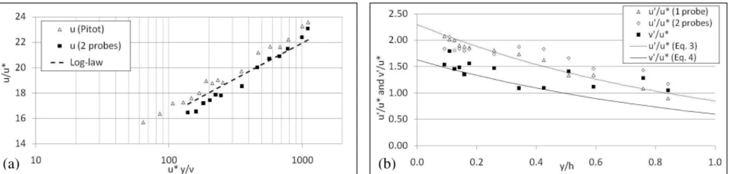
Figure 6. 2D Velocity vertical profile in the middle of the flume (a) and turbulence intensities (b)
(Parameters: c = 1480 m/s, number of cycles: 2, number of repetitions: 256, Noise level: 6, Maximum depth: 109.89 mm, Velocity range: [–0.623;
0.618] (m/s), number of samples: 2100, Start channel: 104.99 mm, End channel: 108.32 mm, Channel width: 0.37 mm).
In Figure 6a the results obtained using the Pitot tube and the results computed with the log-law proposed with B = 5.1, are also presented for comparison. Computing the friction velocity with the Clauser’s method, as in the previous section, one obtains u* = 0.0236 m/s and B = 5.03 for the two UVP probes set-up. The results show a reasonable agreement with the log-law, although the two probes set-up seems to give slightly lower streamwise velocities than the Pitot tube.
Analyzing hot-film anemometry data, Nezu and Nakagawa (1993) recommended the following exponential laws to express the turbulence intensities in the streamwise, u’, and in the cross-wise, v’, directions.
(
)
* '
2.30 exp
u
y h
u = −
(3)
(
)
* '
1.63exp
v
y h u = −
(4)
Equations (3) and (4) are shown in Figure 6b where the streamwise (obtained with one and two probes) and transverse turbulence intensities are presented. The results show a good agreement of the streamwise turbulence intensity obtained with one and two probes. The transverse turbulence intensity has a worse agreement with the exponential law of Nezu and Nakagawa (1993), especially in the outer layer (y/h > 0.4).
CONCLUSIONS
A set of experiments was performed in order to evaluate the quality and precision of the measurements with a UVP system in a open-channel flow. For this analysis, different configurations (cf. Figure 2) and different seeding conditions were used. For diagonal positioning of the probe it was not possible to obtain accurate vertical profiles of the
streamwise velocity. Even using different particles as seeding added to the water, the results were not correct, revealing effects of reflections from the channel bottom.
For horizontal positioning of the probe the results from different tests (changing the start and end channel and the channel width) showed that a weaker echo coming from the particles distant from the probe generates not only a reduction in the velocity values but also some scatter. Nevertheless, the results near the probe remain accurate without significant differences between the measurements taken with different parameters.
Regarding the influence of seeding conditions, the depth and cross-section averaged results showed good agreement, irrespective of the type of seeding condition. The log-law was successfully fitted to the values of the vertical profile of time averaged velocity in the axis of the flume. The values obtained for friction velocity u* and for constant B are sensible to seeding conditions, being the best results obtained with crushed nut shell that has a diameter slightly higher than the theoretical minimum diameter.
By crossing two probes, the 2D velocities profiles and the turbulence intensities were obtained revealing reasonably good agreement with analytical exponential laws.
REFERENCES
Biron, M.B.; Robson, C.; Lapointe, M.F.; Gaskin, S.J. (2004) – “Comparing different methods of bed shear stress estimates in simple and complex flow fields”. Earth Surface Processes and Landforms, 29: 1403-1415.
Bombar, G.; Kantouh, S.; Albayrak, I. (2008) – “Comparison of ADVP and UVP in terms of velocity and turbulence measurements in a uniform flow” RiverFlow 2008, Int. Conf. on Fluvial Hydraulics, Izmir, Turkey, Vol. 1, pp. 281-288. Cardoso, A.H. (1990) – “Spatially accelerating flow in a smooth open channel”. National Laboratory for Civil
Engineering. Memory n. 759.
Coles, D. E. (1968) – “The young person's guide to the data”. Proc. comput. turbulent boundary layers — AFOSR-IFP-Stanford Conference, (eds. Coles, D. E.; Hirst, E. A.). Vol. 2, pp. 1–46. Dept. Mech. Eng., AFOSR-IFP-Stanford University. Goring, D. G.; Nikora, V. I. (2002) – “Despiking acoustic Doppler velocimeter records”. Journal of Hydraulic Engineering, ASCE 128: 117-126.
Kantoush, S.A.; De Cesare, G.; Boillat, J.L.; Schleiss, A.J. (2008) – “Flow field investigation in a rectangular shallow reservoir using UVP, LSPIV and numerical modelling”. Flow Measurement and Instrumentation, 19, 3-4: 139-144. Manes, C.; Pokrajac, D.; McEwan, I.; Nikora, V.; Campbell, L. (2006) – “Application of the UVP within porous beds”. Journal of Hydraulic Engineering, ASCE, 132: 983-986.
Metflow (2002) – “UVP Monitor Model UVP-DUO - Users guide”. Metflow SA, Lausanne, Switzerland. Nezu, I.; Nakagawa, H. (1993) – “Turbulence in Open-Channel Flows”, IAHR-Monograph, Balkema.
Ozaki, Y.; Kawaguchi, T.; Takeda, Y.; Hishida, K.; Maeda, M. (2002) – “High time resolution ultrasonic velocity profiler”. Experimental Thermal and Fluid Science, 26: 253-258.
Sato, Y.; Mori, M., Takeda; Y, Hishida, K.; Maeda, M. (2002) – “Signal processing for advanced correlation ultrasonic velocity profiler”. Third International Symposium on Ultrasonic Doppler Methods for Fluid Mechanics and Fluid Engineering EPFL, Lausanne, Switzerland, September 9 - 11, 2002.Takeda, Y. (1995) – “Velocity Profile Measurement by Ultrasonic Doppler Method”. Experimental Thermal and Fluid Science, 10: 444-453.
Takeda, Y.; Kikura, H. (2002) – “Flow mapping of the mercury flow”. Experiments in Fluids, 32: 161-169.
Vanoni, V.A.; Brooks, N.H. (1957) – “Laboratory studies of the roughness and suspended load of alluvial streams”, California INstitue of Technology Lab. Rep., no E-68, California
Wiklund, J. A.; Stading, M.; Pettersson, A. J.; Rasmuson, A. (2006) – “A Comparative Study of UVP and LDA Techniques for Pulp Suspensions in Pipe Flow”, American Institute of Chemical Engineers Journal 52, 484-495.
ACKNOWLEDGMENTS