Aerial Semantic Mapping for Precision Agriculture using Multispectral Imagery

(1)

Ana Beatriz de Tróia Salvado

Licenciado em Ciências da Engenharia Electrotécnica e de Computadores

Aerial Semantic Mapping for Precision

Agriculture using Multispectral Imagery

Dissertação para obtenção do Grau de Mestre em

Engenharia Electrotécnica e de Computadores

Orientador: Prof. Dr. José António Barata de Oliveira, Prof. Associado, Universidade Nova de Lisboa

Co-orientador: Mestre Ricardo André Martins Mendonça,

Investiga-dor, Universidade Nova de Lisboa

Júri

Presidente: Prof. Dr. Luís Augusto Bica Gomes de Oliveira, FCT-UNL Arguente: Prof. Dr. José Manuel Matos Ribeiro da Fonseca, FCT-UNL

(2)

(3)

Aerial Semantic Mapping for Precision Agriculture using Multispectral Imagery

(4)

(5)

(6)

(7)

Acknowledgements

"Unity is strength... when there is teamwork and collaboration, wonderful things can be achieved." - Mattie Stepanek

Sharing moments, in a life full of daily routines, hard-work and commitment becomes true gold when it comes to find the right balance in life. Working together is the unity of growing with new ideas, solutions and knowledge to reach success. Family and Friendship is the magical formula to turn everything into happiness, laugh and crazy adventures, shaping who we are and the way we live. For this reason, I would like to leave a special "Thank You" to each person who crossed my path during this wonderful journey of learning.

I would like to thank Faculdade de Ciências e Tecnologias from Universidade Nova de Lisboa, for being my second home for the last five years. A peaceful place full of so many good people and which location allowed quick getaways to the coast with a wonderful view over the sea.

A special thank you to professor José Barata for being such an enthusiastic and wel-coming person. Motivating us to dive into a wide range of opportunities and new projects full of innovation and technology. Thank you very much for letting me be part of RICS group, a team full of bright minds and personalities who, not only shared their lab with me, but also for the companionship, joy and playing moments, in a place where it is possible to work in a valuable environment, feeling the achievements of each other and progressing as a group.

Thank you Ricardo Mendonça, not only for the support and advice during all this working project but also for the leisure moments you provided everyday in that room, sharing your playlists in the RICS lab, by making it into a lighter environment with your great taste for background music. It was also a pleasure to share this lab with Francisco Marques, André Lourenço, Eduardo Pinto, Carlos Simões, Manuel Silva, Pedro Prates, João Lopes and Luís do Ó, who were always there to share their support, experience and guidance, to turn this project idea into reality.

(8)

or David’s drums. For all the evenings and projects that fomented the connection we have today. And also to my friends and companions who also left their footprint throughout this academic journey with me: Gisela, Prego, Sofia Pereira, Rita, Rúben, Rodrigo, Estevam, Andreia, Catarina and all the NEEC members.

Ponto Zero, a second family that I have the pleasure to be part of, for so many years: a team, a place, a gym, a group; sharing together not only the essence of gymnastics, but also the amazing moments of creativity, laugh and mutual help. Those goosebumps and nervous feeling before getting on stage, exhibitions and all the travels representing our country abroad. A huge thanks to my coaches João Martins and Pascoal Furtado for being in my life with such strong personalities, from whom I learnt so much and grew as a person.

Last but not least, thank you so much to my family and close friends, to my grandparents and godparents who always believed in me to achieve so much. But specially to my wonderful Mum who is always there for the best conversations, advice and contagious smile; to my dad not only for being a man always ready to share his wisdom with his daughters but also for his valuable serenity solving problems, playful mind and jokes; A huge "Thank You!" to my big sis Ana Rita, that despite all the challenges we go through, is always there to cheer me up, to give me such support whatever it takes and to give me all the strength to follow my dreams; and to João Pedro Carvalho, whose smile brightens up my life everyday, for all his love and positivism, believing that everything is possible.

(9)

A b str act

Nowadays constant technological evolution cover several necessities and daily tasks in our society. In particular, drones usage, given its wide vision to capture the terrain surface images, allows to collect large amounts of information with high eﬃciency, performance and accuracy.

This master dissertation’s main purpose is the analysis, classification and respective mapping of diﬀerent terrain types and characteristics, using multispectral imagery.

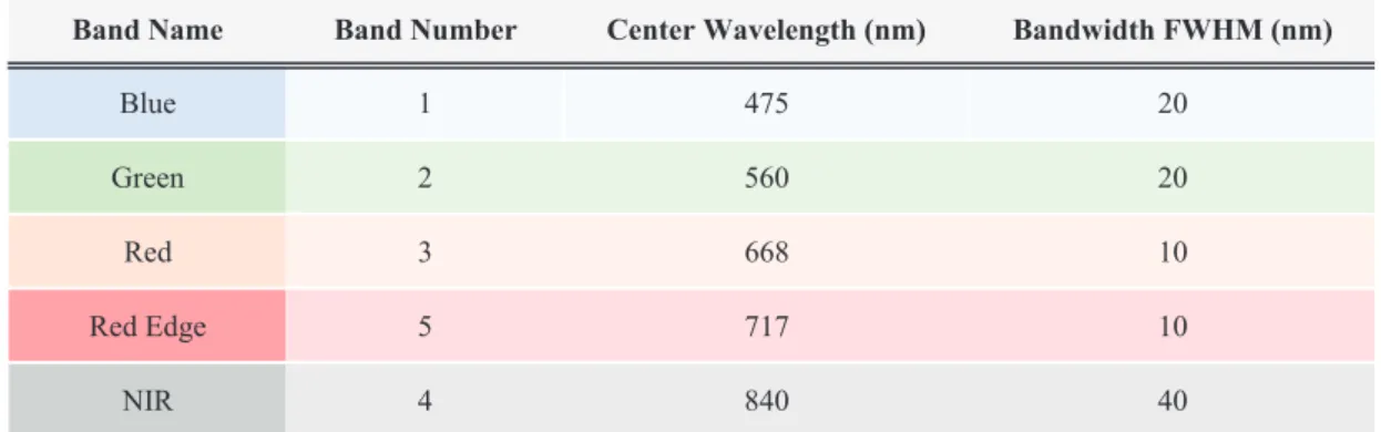
Solar radiation flow reflected on the surface is captured by the used multispectral camera’s different lenses (RedEdge-M, created by Micasense). Each one of these five lenses is able to capture different colour spectrums (i.e. Blue, Green, Red, Near-Infrared and RedEdge). It is possible to analyse the various spectrum indices from the collected imagery, according to the fusion of different combinations between coloured bands (e.g. NDVI, ENDVI, RDVI. . . ).

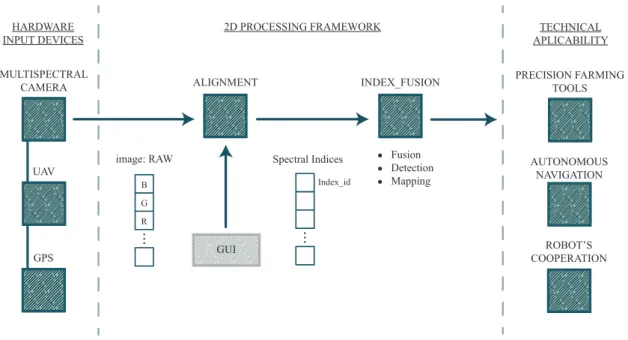
This project engages a ROS (Robot Operating System) framework development, ca-pable of correcting diﬀerent captured imagery and, hence, calculating the implemented spectral indices. Several parametrizations of terrain analysis were carried throughout the project, and this information was represented in semantic maps by layers (e.g. vegetation, water, soil, rocks).

The obtained experimental results were validated in the scope of several projects incorporated in PDR2020, with success rates between 70% and 90%.

This framework can have multiple technical applications, not only in Precision Agri-culture, but also in vehicles autonomous navigation and multi-robot cooperation.

(10)

(11)

R e su mo

A constante evolução tecnológica cobre, hoje em dia, diversas necessidades e tarefas diárias da nossa sociedade. Particularmente, a inserção de drones, dada a sua ampla visão para captar imagens sobre a superfície do terreno, permite a recolha de grandes quantidades de informação com grande eficiência, desempenho e precisão.

A presente dissertação de mestrado tem como principal objetivo a análise, classificação e respetivo mapeamento de diferentes tipos e características de terrenos a partir de imagens multiespectrais.

O fluxo de radiação solar refletida pela superfície é captado pelas diferentes lentes da câmara multiespectral utilizada (RedEdge-M, produzida pela Micasense). Cada uma das cinco lentes é capaz de captar diferentes espectros de cor (i.e. Blue, Green, Red, Near-Infrared e RedEdge). A partir das imagens recolhidas é possível analisarem-se diversos índices espectrais consoante a fusão de distintas combinações entre as bandas de cor (e.g. NDVI, ENDVI, RDVI. . . ).

Este projeto passa pelo desenvolvimento de uma nova framework em ROS (Robot Operating System) capaz de corrigir as diferentes imagens captadas e consequentemente calcular os índices espectrais implementados. Foram realizadas diversas parametrizações ao longo do projeto para a análise de terrenos, cuja informação é representada em mapas semânticos por camadas (e.g. vegetação, água, solo, rochas).

Os resultados experimentais obtidos foram validados no âmbito de vários projetos inseridos no PDR2020, com taxas de sucesso compreendidas entre 70% e 90%.

Esta framework poderá ter diversas aplicações técnicas não só na Agricultura de Pre-cisão, como também para a navegação autónoma de veículos e ainda na cooperação multi-robot.

(12)

(13)

Conte nts

List of Figures xv

List of Tables xvii

Acronyms xix

1 Introduction 1

1.1 Context and Motivation . . . 1

1.2 Goal and Approach . . . 2

1.3 Dissertation Structure . . . 3

2 State of the Art 5 2.1 Challenges in Modern Agriculture . . . 5

2.1.1 Fruit’s Biofortification in Agriculture . . . 7

2.1.2 Alternative Application Systems to Prevent Over-Fertilization Issues in Agriculture . . . 7

2.2 Remote Sensing in Precision Agriculture . . . 9

2.2.1 The Application of Unmanned Aerial Systems in Precision Agriculture 10 2.2.2 Multispectral Sensing . . . 12

2.3 Image Processing and Aerial Mapping in PA . . . 20

2.3.1 Image Stitching and Mosaicking . . . 21

3 Supporting Concepts 25 3.1 Frameworks and Computer Vision . . . 25

3.1.1 ROS . . . 25

3.1.2 OpenCV Library . . . 26

4 Proposed Framework 29 4.1 Model Overview . . . 29

4.2 Hardware Infrastructures . . . 31

4.2.1 Unmanned Aerical Vehicle . . . 31

4.2.2 Micasense Multispectral Camera . . . 33

4.2.3 Imagery Type and Metadata . . . 35

(14)

C O N T E N T S

4.2.5 Lenses Alignments . . . 41

5 Framework Implementation 43 5.1 ROS-based Architecture . . . 43

5.1.1 Service Triggering Operations . . . 44

5.1.2 ROS Messages . . . 45

5.1.3 RedEdge-M Communication Node . . . 46

5.2 Online and Oﬄine Missions - User Interface . . . 47

5.3 Image Metadata Extractor . . . 47

5.4 Reflectance Conversion . . . 48

5.4.1 Converting Raw Images to Radiance . . . 48

5.4.2 Panel Detection and Calibration . . . 49

5.4.3 RedEdge-M Lens Distortion Corrections . . . 51

5.5 Image Alignment . . . 53

5.5.1 Alignment Algorithm . . . 53

5.5.2 Image Alignment Node . . . 56

5.6 Index Fusion . . . 58

5.6.1 Spectral Indices Computation . . . 59

5.6.2 Terrain Classification . . . 59

5.6.3 Semantic Layer Mapping . . . 60

6 Experimental Results 65 6.1 Experimental Setup . . . 65

6.2 Model Parametrization . . . 66

6.3 Experimental Datasets . . . 66

6.4 Results Validation . . . 68

6.4.1 Colour Band Alignments . . . 68

6.4.2 Terrain Classification Assessment . . . 69

7 Conclusions and Future Work 73 7.1 Conclusions . . . 73

7.2 Future Work . . . 74

Bibliography 75 A Rededge-M Imagery Sensor 79 A.1 Sample of a YAML metadata file from Rededge-M Imagery Sensor . . . . 79

B Terrain Classification Results 85

(15)

Li st o f F i g u r e s

2.1 Forecasted agricultural needs due to population growth, in 2050. . . 5

2.2 Proportions of micronutrient deficient soil in China. . . 7

2.3 Eﬃciency gains and application costs . . . 8

2.4 Examples of UAV: Powered glider and Parachute . . . 10

2.5 Examples of UAS: Fixed-wing aircraft and RC-Helicopters . . . 11

2.6 Examples of small UAV: weControl helicopter and quadcopter micro-UAV . . 12

2.7 The concept of imaging spectroscopy. . . 13

2.8 Satellites used as multispectral imagery acquisition sensors . . . 14

2.9 Reflectance spectrum of a typical green leaf . . . 16

2.10 Software orthomosaicking results with Pix4D, APS and Photoscan . . . 22

2.11 Big O notation. . . 23

4.1 Aerial vehicle navigation plan. . . 29

4.2 General work proposed structure. . . 30

4.3 Cooperation between autonomous systems. . . 31

4.4 Orthophoto georeferenced layers. . . 31

4.5 Unmmaned aerial vehicle infrastructure. . . 32

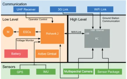
4.6 UAV hardware layer’s communication’s achictecture. . . 32

4.7 Micasense spectrum transmisivity curves. . . 33

4.8 Micasense sensors integration. . . 34

4.9 UAV infrastructure . . . 35

4.10 Reflectance curves of snow, vegetation, water, and rock. . . 38

4.11 Calibration panel captured by the RedEdge-M NIR sensor. . . 39

4.12 Radiometric calibration with multi-panels integration. . . 40

5.1 ROS implemented infrastructure’s diagram. . . 44

5.2 Calibration’s panel-base image with the QRcode and radiance square. . . 49

5.3 Panel Detection: example of an homography good matches result. . . 50

5.4 Radiance square detection diagram. . . 50

5.5 Camera Model’s Calibration. . . 52

5.6 Radiometric calibration with multi-panels integration. . . 53

5.7 Misalignments between scene images from diﬀerent lenses. . . 54

(16)

L i s t o f F i g u r e s

5.9 Example of the OpenCV library algorithm: Features2D + Homography. . . . 56

5.10 Terrain Layers viewed from the Rviz tool . . . 60

5.11 Unmanned Aerial Vehicle(s) (UAV) pipeline to determine the image plane’s real dimension. . . 61

5.12 Interfaces’ coordinate systems: world,map,base_link and OpenCV. . . 62

6.1 Experimental tests in the field . . . 67

6.2 Rededge-M camera sensor imagery nomenclature. . . 67

6.3 Relative provision between the band filters. . . 68

6.4 Alignments examples. . . 69

6.5 Validation masks. . . 70

6.6 Spectral indices Results. . . 70

6.7 Terrain classification success rate results. . . 71

(17)

Li st of Tab l e s

2.1 Applications of a multispectral sensor band-set . . . 16

4.1 Micasense colour bands wavelength center. . . 33

4.2 Micasense radiometric calibration model. . . 36

5.1 Terrain types parametrization. . . 59

6.1 Terrain classification parametrization. . . 66

(18)

(19)

Acr ony ms

3RT Three Rate Technology.

AGL Above Ground Level.

API Application Programming Interface.

APS Aerial Photo Survey.

AVIRIS Airborne Visible Infrared Imaging Spectrometer.

B boron.

BBA Block Bundle Adjustment.

CARI Chlorophyll Absorption Ratio Index.

CRP Calibrated Reflectance Panel.

CRT Constant Rate Technology.

Cu copper.

DLS Downwelling Light Sensor.

DSM Digital Surface Model.

DTM Digital Terrain Model.

ECC Enhanced Correlation Coeﬃcient.

ENDVI Enhanced Normalized Diﬀerence Vegetation Index.

Fe iron.

FLANN Fast Library for Approximate Nearest Neighbors.

FOV Field of View.

(20)

A C R O N Y M S

GPS Global Positioning System.

GUI Graphical User Interface.

HFOV Horizontal Field of View.

I iodine.

IMU Inertial Measurement Unit.

IOT Internet of Things.

LAI Leaf Area Index.

LWIR Longwave Infrared.

MCARI Modified Chlorophyll Absorption Ratio Index.

Mn manganese.

Mo molybdenum.

MSAVI Modified Soil-Adjusted Vegetation Index.

MSE Mean Squared Error.

MSMS MultiSpectralMicroSensor.

MSR Modified Simple Ratio.

MU Management Unit.

NDVI Normalized Diﬀerence Vegetation Index.

NIR Near-infrared.

OpenCV Open Source Computer Vision Library.

PA Precision Agriculture.

PDR2020 Programa de Desenvolvimento Rural 2014-2020.

PWM/GPIO Pulse Width Modulation/General-Purpose Input/Output.

RC-Helicopter Remotely Controlled Helicopters.

RDVI Renormalized Diﬀerence Vegetation Index.

RE Red-Edge.

(21)

A C R O N Y M S

RGB Red, Green and Blue.

RICS Robotic & Industrial Complex Systems.

ROA Remotely Operated Aircraft.

ROS Robot Operating System.

RPV Remotely Piloted Vehicles.

RTK Real Time Kinematic.

SAVI Soil-Adjusted Vegetation Index.

Se selenium.

SfM Structure From Motion.

SR Simple Ratio.

SWIR Short Wave Infrared.

SWIR-2 Short Wave Infrared 2.

SWIR-1 Short Wave Infrared 1.

TVI Triangular Vegetation Index.

UAS Unmanned Aerial System(s).

UAV Unmanned Aerial Vehicle(s).

VRT Variable Rate Technology.

VTOL vertical take-oﬀ and landing.

(22)

(23)

Nome n cl atu r e

Some of the most common and constant symbols used throughout the thesis are listed below.

Units

g Gram

kg Kilogram

m Metre

cm Centimetre

mm Millimetre

nm nanometre

s second

sr steradian

W watt

MB Megabyte

Gb Gigabit

px Pixel

E Irradiance

(24)

(25)

C

h

a

p

t

e

r

1

Intr o d u cti on

1.1 Context and Motivation

In today’s world, technology is increasingly becoming part of human life; in an environment where data acquisition is an issue in our community since information is continually growing and changing. People no longer need to learn how to adapt to innovation but instead technology is responsible for modelling itself around society; by processing all the sensor’s acquired information, getting results, conclusions and even learning how to behave even when faced with unknown situations.

Technology enhancement is embracing society, not only by learning how to adjust itself to each individual and their own personal devices, but also by reaching various industrial sectors in great scale. Fields of operation where UAV can give a huge contribution, achieving as much information as possible in the least possible time about any Big Data systems, such as traﬃc surveillance, security and rescue operations, building inspections, mapping or even agricultural monitoring.

Nowadays, one of the biggest concerns in our society is related to both food and water security, as well as well-nourished population assurance, which involves selling food that provides the major nutrients to preserve a healthy society.

This thesis’ concept urged from various projects related to fruit and cereal cropping fields, technologically arising in partnership with Faculdade de Ciências e Tecnologias (FCT-UNL), such as:

• MPBIO – GO Biofortificação de Tomate para Processamento Industrial e em Modo de Produção Biológica (Biofortification of Tomato with Mg, Zn e Fe) – Project Number PDR2020-101-030701, 01 Ação 1.1/2016, Initiative nº 6, Partnership nº 11;

(26)

C H A P T E R 1 . I N T R O D U C T I O N

Ca) – Project Number PDR2020-101-030719, 01 Ação 1.1/2016, Initiative nº 20, Partnership nº 17.

• PERCAL – GO Biofortificação de Pera Rocha em Calcio (Biofortification of Pear with Ca) – Project Number PDR2020-101-030734, 01 Ação 1.1/2016, Initiative nº 148, Partnership nº 76.

• UVAZN – GO Fortificação de uva em zinco para vinho branco e tinto (Biofortification of Grapes with Zn) – Project Number PDR2020-101-030727, 01 Ação 1.1/2016, Initiative nº 144, Partnership nº 74.

• INSTAGRI - Intelligent Cloud Based Environment for Precision Agriculture using Remote Sensing Technology – Project Number CENTRO-01-0247-FEDER-023152.

The previously mentioned projects rely on new Portuguese motivational researches of an agricultural change in the country. It has been gradually growing in Portugal for several years, through national companies like Syngenta or Wisecrop, already with creative and eﬃcient developed solutions in the market. They use techniques based on aerial multispectral captured images of the field area, capable to gather information invisible to human eye, in order to advise farmers about their crops growth, indicating possible plagues, diseases or even fields’ malnutrition.

1.2 Goal and Approach

Despite the distinct techniques taken by diﬀerent entities on the agricultural business, this thesis proposes an open-source framework development for precision agriculture that will be fully integrated with an UAV, which is the main asset responsible for the agricultural field autonomous scanning.

With the use of an incorporated multispectral RedEdge-M camera, developed by Mi-casense, the UAV intends to collect a full real-time imagery dataset of the cultivation area, which will provide five diﬀerent colour spectrum bands for each taken frame: Red, Green, Blue, Infrared and Red-Edge.

Furthermore, it should allow an index fusion between the bands and the information collected by the camera using the Open Source Computer Vision Library (OpenCV), a ma-jor tool for image and video analysis. The multispectral imagery eﬀects over the overflown area ground type will provide feasible information about possible terrain irregularities, obstacles or target fertilization points, for instance. Thus, the imagery revealed features will be compiled into a layered map with certain areas labelled according to the terrain type detected. This will then be fused into an occupancy map, in order to support the UAV autonomous navigation in constrained environments.

This thesis analysis and monitoring system goal is supported with the ability to interpret the diﬀerent eﬀects caused on each captured field area’s colour band, due to the type of terrain features.

(27)

1 . 3 . D I S S E RTAT I O N S T R U C T U R E

This approach intends to improve the acquired knowledge about Precision Agriculture, as well as autonomous navigation and multi-robot cooperation. It is an opportunity to share and enhance the Robotic & Industrial Complex Systems (RICS) research group with the explored and developed material about the field. Therefore, this dissertation is focused on analysing and enriching the usage of Multispectral cameras in this industry.

1.3 Dissertation Structure

This dissertation presents a fully integrated system for terrain classification and mapping. It is organized into 6 chapters along with this section, starting from the state-of-the-art review until the actual project implementation and it’s final statements and conclusions:

• Chapter 1: Introduction presents the project and main goals to achieve with terrain classification and mapping, as well as multiple projects that motivated this thesis’ development;

• Chapter 2: State of the Art shows the UAV usage background around agricultural

sector and the multispectral imagery evolution throughout history, reaching nowadays drones advantages in daily tasks;

• Chapter 3: Supporting Concepts enrols the reader with basic technology concepts

integrated in this project;

• Chapter 4: Proposed Framework describes the framework and introduces the infras-tructures applied in the scope of this project;

• Chapter 5: Framework Implementation details the implementation steps;

• Chapter 6: Experimental Results includes the model parametrization and testing, containing the output results, their validation and analysis;

• Chapter 7: Conclusions and Future Work sums up all the implemented strategy, challenges, future developments and suggestions to improve the algorithms and project ambitions;

• Appendix A: Rededge-M Imagery Sensor Sample of a YAML metadata file from

Rededge-M Imagery Sensor;

(28)

(29)

C

h

a

p

t

e

r

2

S tate of th e A r t

2.1 Challenges in Modern Agriculture

Nowadays, with environmental change, it becomes challenging for society to embrace smarter ways for crop improvement or water and fertilizers control. Underdeveloped countries are increasingly facing agricultural salinity and waterlogging problems due to the lack of irrigation management. This same lack of water issues are starting to manifest crop production limitations in developed countries [1].

According to David Tilman, it was studied that in approximately 30 years the popula-tion will increase 35%, meaning that crops’ producpopula-tion should double [2]. Besides, growth in demand for protein food is also a concern since the pace of production must overcome the demographic growth (Figure 2.1).

Least developed countries Developing countries Developed countries

103,6% 15,3%

69,2%

35%

Population Growth

Crops Production

World Demand for Protein Food 100%

(30)

C H A P T E R 2 . S TAT E O F T H E A RT

According to [2] agricultural nourishing issues can be mitigated or even eradicated by taking the following 5 actions:

1. Stopping Agriculture’s climate footprint _→ Preventing deforestation when building new farms;

2. Harvesting increase in the existing farmlands → Enhancing farms’ production by

adopting new technological systems capable to accurately adjust the use of fertilizers and pesticides;

3. Ensure a greater eﬃciency of the resources →Agricultural practices using resources

capable to adjust according to the field characteristics and state of production;

4. Diet change_→Since, only 55% of the crops’ calories are ingested by humans, whereas the rest goes to cattle, biofuels and industrial products, it would be ideal to change some population food habits. However, this is considered an almost impossible measure to fulfill, which therefore leads to the adoption of nourishment crops for the production of bio-fuels as a solution to enhance food availability;

5. Reducing the food waste → Minimizing the loss of food before consumption not

only in the developed countries where there is an avoidable excess of wasted food at supermarkets, restaurants and residences, but also at the least developed countries where the products loss due to transportation issues is still too high.

Regardless, food consumption still grows according to the associated population in-crease, as well as urbanization considers people’s preference on moving from their rural livelihoods to bigger urbanized cities. Both issues are correlated since urbanization limits food production, which therefore leads to tropical forests’ destruction aiming to increase the cultivable soil.

Agriculture is one of the main causes for global warming due to deforestation (which secures biodiversity and natural carbon cycle) and greenhouse gas emission that represents proportions even bigger than cars, trains or aircraft emissions [2]. It is critical to find a solution for crops’ production increase within the limited land available and water usage restrictions for environmental causes. Besides, reducing energy consumption is a necessity as well, such as the continuous food production taking into account the inevitable climate change impacts already caused [1].

On the other hand, along with the food production it is also very important to keep the high nourishment levels; for instance, article [3] studies the nutritional deficiency at China’s soil and population, derived from the lack of elements in food (Figure 2.2). As an example, the eminent lack of iron (Fe) evidences itself in the anaemic population increase, sub-clinical deficient levels of boron (B), copper (Cu), manganese (Mn), molybdenum (Mo), zinc (Zn), selenium (Se) or even iodine (I) aﬀects millions of people with goitre

disease.

(31)

2 . 1 . C H A L L E N G E S I N M O D E R N A G R I C U LT U R E

0 10 20 30 40 50 60

B Mn Cu

Mo Se

Fe Zn

Proportions of micronutrient deficient soil in China

% Deficient

Figure 2.2: Proportions of micronutrient deficient soil in China. From [3].

2.1.1 Fruit’s Biofortification in Agriculture

In China, according to [3], 40% of the land is clearly deficient on Zn and Fe, therefore it is critical to find plant nutritional strategies capable of solving these issues. In particular, the biofortification approach is considered sustainable, low-cost and reveals to be eﬃcient increasing the breeding of crops’ micronutrients density and bioavailibility. Since China’s nutritional regime mainly includes tube crops and vegetables, the enrichment of plants, rice, wheat and maize is a priority.

Recently, there were also analysed the agricultural practices with micronutrients’ fertil-izers. On the other hand, article [3] reviews two fertilizer types: soil and foliar application. Despite the major nutritional eﬀects in micronutrients’s density and plant’s bioavailability, it also refers to the drawbacks around the large temporal and spatial recovery due to the fixed plant-unavailable form issue behind soil application fertilizers, and to the ineﬃciency of foliar-applied micronutrients since the plant roots are not usually reached.

Therefore, farming tends to improve with breeding programs’ implementation, field drainage and a better fertilizer technological strategies usage. Indeed, it is critical to reduce the over-fertilization and pesticides usage to lower the global greenhouse gas emission levels, the degrading of water resources or even farmland and aquatic ecosystems impacts [1].

2.1.2 Alternative Application Systems to Prevent Over-Fertilization Issues in

Agriculture

Variable Rate Technology (VRT), Site-Specific Farming or Precision Agriculture are some of the nomenclatures given to the optimal fertilization supplement that instead of being a nutrients’ single rate based process (Constant Rate Technology), it will be able to accordingly adjust itself to each location needs (Multiple Rate Technology) [4].

(32)

2.1.2.1 Implementation’s Economic Feasibility/Viability (Business Case)

The eﬃciency impacts of this nutrients non-waste process are remarkable, however the article [4] reveals an interesting study of nitrogen fertilization on corn that answers to the real question around VRT investment: the balanced trade-oﬀ between the revenues and the costs of application involved. In order to proceed with this study, it also took into account the Constant Rate Technology (CRT) and the Three Rate Technology (3RT) study cases, which provided the ability to compare the net revenues between the three technologies (VRT, CRT and 3RT).

Tests were also made in two distinct types of fields: one area with an average fertility level homogeneous along the whole field, and another area less homogeneous. In other words, whereas field A was spatially homogeneous, field B had a greater soil spatial variability of fertility levels.

Simultaneously, it is a fact that the less fertilized is the field, the greater will be the eﬃciency gain with the CRT method. However, VRT provides a proper nitrogen quantity until a fertility Management Unit (MU) of 1.5m (minimum MU possible).

On the other hand, this area of production detailed analysis requires a certain invest-ment in more complex equipinvest-ment capable of handling smaller manageinvest-ment unit area and greater information volume to be analysed. In return, there is a cost decrease referred to the less wasted fertilizer and yield increase.

CCRT EGCRT EGA 3RT EGA VRT C3RT CVRT EGB 3RT EGB VRT EGB EGA COST

NCRT= 1 N3RT= FL/100 NVRT= FL/1.5

S_CRT= FL S_3RT= 100 S_VRT= 1.5

Size of Management Units (S) Number of Management Units (N)

Field B

- High Var iability

Field A - Low Variability

$/ha

Figure 2.3: Eﬃciency gains (EG) and application costs (C). Graph adapted from [4].

(33)

2 . 2 . R E M O T E S E N S I N G I N P R E C I S I O N A G R I C U LT U R E

Although the positive results revealed in the article due to the studied methods’ eﬃ-ciency gains versus associated costs (Figure 2.3), the CRT method was more profitable in small fields with an homogeneous fertility than VRT because when there is a field with an average fertility high but with a low variability, it means that more areas require the maximum possible rate of fertilizer which will therefore generate the best yield gain. Furthermore, the revenues of implementing a VRT system under the previous conditions wouldn’t be suﬃcient to cover the application costs.

Nevertheless, the multiple rate technology (VRT) was more profitable in most of the scenarios in study, with larger net revenues than CRT or 3RT, and besides, environmental benefits of VRT were notable as the variability of the studied area’s fertility increased comparing to the CRT environmental impacts due to the excess of fertilizer in use.

2.2 Remote Sensing in Precision Agriculture

Precision Agriculture (PA) is a technology that has been gradually growing over the years, beneficing farmers who need to regularly manage their agricultural fields. The application of several sensors, strategically placed and distributed over the field was a step-forward into the autonomous analysis of terrains, since it became possible to detect the field changes and retrieve feasible information about its state of production nearly in real-time.

Correlation between multi-spectral imagery and geospatial information from a Global Positioning System (GPS) or a Geographic Information System (GIS), was pivotal to foster the evolution of this technology. It allowed mapping between the image data and the geographical location of its acquisition (i.e. image georeferencing). However, only with the appearance of remote sensors with enough quality and reasonable costs, arose the opportunity to finally invest in the agricultural sector, since until then the only collected imagery data used for this purpose mostly came from satellites, which had high-resolution, but were an expensive approach, as well as limited accessibility.

Remote sensing applications in PA are also able to regularly provide farmers feasi-ble information about their field, which can possibly reveal critical crop conditions still non-detectable by human eye but technologically collected in advance through complex equipment. The multispectral imagery output will indicate diﬀerent index values at the distinct bands, from which data analysis can reveal diﬀerent meanings about the crops growing state.

Therefore, remote sensing grant a better agricultural monitoring and the possibility to take actions in a timely manner in order to accordingly adjust the undertaken procedures and prevent associated losses [5].

The article [5] also refers the four diﬀerent stages of PA process:

(34)

2. Mapping → field variation, crop-type, tillage, crop residue and yield mapping;

3. Analysis and decision making_→ calculate the finest imagery acquisition frequency, control the fertilizer quantities and other decision making procedures;

4. Performance management _→ intervention over the plans and established implemen-tations to correct the farming methods under process [6].

According to [5], remote sensing could autonomously be responsible for the previously mentioned first three PA steps, eﬃciently collecting large amounts of data from extent agricultural fields within a short period of time.

Along with the expansion of multispectral technology and data fusion, there are various monitoring applications arising that, not only take near real-time farm analysis as a priority, but also motivate the environmental care within the agricultural sector.

2.2.1 The Application of Unmanned Aerial Systems in Precision Agriculture

At the moment, VRT combined with GPS is one of the most advanced technologies in precision agriculture, but for its entirely success, as previously stated, complex equipment and high quality sensors are required in order to capture detailed maps of the entire field in study and capable to accurately detect possible plagues, diseases or malnutrition.

Unmanned aerial systems are the main competitors in the market against satellites’ imagery acquisition due to its accessibility eﬃciency (e.g. daily or even near real-time mon-itoring), detailed resolution (e.g. centimetres) and reasonable costs involved. Unmanned Aerial System(s) (UAS) empower privileged views over the crops and passiveness against weather conditions (e.g. clouds or fog), unlike satellites or manned aircraft.

At the beginning, the exploring and investigation around UAV - vehicles without on-board control - for photometric purposes, started by implementing kites, blimps and balloons, but despite the lower costs involved, they were too big and therefore consid-ered diﬃcult platforms to maneuver. Accordingly, smaller vehicles became desirable, for instance Remotely Piloted Vehicles (RPV) and Remotely Operated Aircraft (ROA).

a b

Figure 2.4: Radio-controlled UAV used in [7] to test the agility and flight constraints of the vehicles in study: (a) L’Avion Jaune’s powered glider, (b) Pixie motorized parachute.

(35)

In article [7], two diﬀerent kinds of vehicles are mentioned for testing their manoeu-vrability (figure 2.4), flight restrictions and abilities to accurately capture multispectral imagery data from the crops. They were both incorporated with digital photographic cameras capable to extract the visible and near-infrared bands from the spectral filters in use.

Nevertheless, the previous study revealed that UAV require lower altitudes during flights to achieve higher spatial resolutions, which means that there may be more instability and vulnerability when acquiring diﬀerent resolutions and distinct viewing angles between the shooting images. This can possibly be corrected by warping the collected pictures based on each georeferenced information.

In article [8] a ground classification of a certain field in Mexico was produced using a fixed-wing aircraft to capture the imagery, using an incorporated frontal video camera at the nose of the UAV and a digital camera at the aircraft’s left wing (Figure 2.5 (a)).

On the other hand, article [9] enhances this thesis with an historical research about RC-Helicopters. [9] not only points to the photogrammetry problems due to the UAV vibrations caused by the rotors, but also considers the GPS accuracy as a solution.

a b

Figure 2.5: (a) Fixed-wing aircraft (BAT 3 UAS), from [8]. (b) Remotely Controlled Helicopters (RC-Helicopter) by Helicam and weControl, Switzerland, from [9].

Even so, unmanned helicopters are valuable covering small terrains and the costs involved are even lower than aircraft investment.

Recently studies around UAV in PA were taken in the agronomic R&D plant of Syngenta Crop Protection AG in Stein (Canton AG, Switzerland). The MultiSpectralMicroSensor (MSMS) project was divided into two phases where the main goal was to research about light-weight multispectral sensor’s prototype incorporated with two distinct UAV: firstly with an autonomous mini-helicopter developed by weControl and then with a micro-UAV.

(36)

a b

Figure 2.6: (a) Helicopter based Mini-UAV by weControl (Zurich), from [10]. (b) Quad-copter micro-UAV ’microdrones md4-200’, from [10].

The quadcopter in Figure 2.6 (b) was favoured in respect to the one represented in 2.6 (a), not only due to its lower weight and cost attributes, but also to its vertical take-oﬀ and landing (VTOL) capability, giving a huge stability eﬀect to the flight, which in turn improves the quality of the captured images.

2.2.2 Multispectral Sensing

When it comes to multispectral sensing subject, it is important to be aware of the diﬀerent concepts around illumination in order to understand a few but very important details about the terms in use, described in [11]:

• Irradiance→ Refers to the light energy emitted into the surface area, per time unit.

Measured in watts per square meter (W/m2₎

• Reflectance→ It refers to values ranged between 0 and 1 to characterize the incident

light reflected by a surface. This fractionated value can be parametrized into distinct variables such as the reflected light wavelength or even the incidence and reflection angles.

• Radiance→ It is a normalized value of the irradiance intensity according to a certain

solid angle, typically specified in steradians (sr) and accordingly variable with the light’s propagating direction. Typically measured in W/m2_{/sr, but when related to} the spectral domain it may be measured in line with the wavelength W/m2_/sr/μm.

According to [11], there are several ways to contactlessly acquire information about a cer-tain object or scene, relying on the sunlit reflected light detected by electro-optical sensors capable of measuring the diﬀerent wavelengths within the visible spectrum: Panchromatic band (i.e. grayscale) or colour imaging sensors (i.e. Red, Green and Blue (RGB)). Besides, there are also thermal sensors, that instead of being light-based, they acquire information relying on the body temperature emissions (i.e. Longwave Infrared (LWIR)).

Nevertheless, there has been an imaging evolution starting to spread its horizons into new bands apart from the RGB and the grayscale domains, by adding for instance, NIR and Short Wave Infrared (SWIR) bands which, when fully integrated and studied together

(37)

may result in valuable information about characteristic object properties according to its molecular composition, diﬀerently exposed through the electromagnetic spectrum.

Therefore, it is possible to achieve some conclusions from multispectral cameras’ ac-quired images such as revealing the type of material from which it is composed or, at least, distribute the objects in scene by groups, relying on their material classification properties. However, in order to take full advantage of the available bands, multispectral imag-ing gets through a spectral processimag-ing, also know as spectroscopy that encompasses the measurement, analysis and finally the result’s interpretation, which can possibly reveal valuable information about the scene in analysis, [11]. On the other hand, when it comes to large scale areas, it is called imaging spectroscopy, as illustrated bellow in Figure 2.7.

Spectral images taken simultaneously

Wavelength

Vegetation Water

Soil

Each pixel contains a sampled spectrum that is used to identify the materials present in the pixel by their reflectance Swath width Spe ctr al dimension Along-tr

ack dimension built up

by the motion o f the space

craft

Earth surface

Spaceborne hyperspectral sensor

Swath width of imaging sensor Re fle ctance Wavelength Wavelength Re fle ctance Re fle ctance

Figure 2.7: The concept of imaging spectroscopy. Illustration from [11].

Imaging spectroscopy retrieves some samples from the ground-based scene where each pixel from the processed image corresponds to the reflectance measured value of the exploited area. For example, in Figure 2.7 the graphs on the right represent diﬀerent spectral variances between the surfaces encountered in the scene, in this case: soil, water and vegetation; from which it was possible to classify the type of terrain, [11].

(38)

the terrain conditions along the years. Figure 2.8 (a) represents Landsat 5 satellite from which 1989 imagery was collected, and Figure 2.8 (b) shows Landsat 7 satellite that later obtained the dataset from 2002 and 2005.

a b

Figure 2.8: Satellites used as multispectral imagery acquisition sensors in [12]. (a) Landsat 5, from [13] and (b) Landsat 7, from [14].

In this research example there were only used five of the seven available bands of the spectral domain: Green-Band, Red-Band, Near-Infrared, Short Wave Infrared 1 (SWIR-1) and Short Wave Infrared 2 (SWIR-2). However, although never used in [12], Landsat 7 could already provide information within the thermal band (band 6 Spatial Resolution: 60 m/pixel), the panchromatic band of the electromagnetic spectrum (band 8 Spatial Resolution: 15 m/pixel) and the spectral Blue-Band (band 1), with a spatial resolution of 28.5 m/pixel, similarly to the ones in use.

Furthermore, article [15], also enhances the spaceborne sensor-based studies with new spectral imagery researches about vegetation classification, which beyond the Landsat TM, also studied other satellites’ datasets such as SPOT-XS, NOAA-AVHRR and IKONOS. From this research there were obtained reasonable results about mapping vegetation species based on the collected Vegetation Indices.

However, in [15], there were described certain sensors’ constraints requiring improve-ments not only related to the limited spatial and spectral sensors’ resolution, but also to the arising questions about the uniqueness of the reflectance spectral properties of a plant, since apart from the specie, there are other variables due to their age, atmospheric and soil growth conditions, topography or plant stresses, for instance.

On the other hand, in 1987, spectral imaging stepped into the hyperspectral domain with the appearance of the first airborne imaging sensor released by NASA Jet Propulsion Laboratory (JPL), the Airborne Visible Infrared Imaging Spectrometer (AVIRIS). Whereas the multispectral domain was limited between 3 to 10 wider bands, the expansion into the hyperspectral domain, with hundreds of narrow available bands, significantly increased the imagery sensors’ accuracy [16].

(39)

The spectral complexity around the AVIRIS’s collected imagery opened up an opportu-nity to distinguish diﬀerent minerals solely based on the Reflectance Spectrum, since each mineral has a diﬀerent molecular constitution possible to detect by the distinct regions where the mineral absorbs the energy, [17]. For instance, as described in article [15], it was possible to distinguish some salt marsh species: Salicornia, Grindelia and Spartina.

Despite hyperspectral systems’ accuracy, they are still an expensive approach and timely-consumer due to the high-resolution processing involved [11].

For that matter, according to [9], in 1980 the first helicopter for photogrammetric purposes appeared, capable of reaching a maximum payload of 3 kg, which means that by attaching cameras such as Rolleiflex SLX or Hasselblad MK 20 it became possible to acquire some aerial imagery from the helicopter.

On the other hand, with the appearance of smaller aerial systems, such as the UAV, and their continuous evolution into becoming increasingly lighter, it also brought the drawbacks related to the vehicle’s possible payload, limited to approximately 20-30% of the system’s total weight [10]. The physical attributes of the multispectral imagery sensors were also a main factor to the continuous study around this science, which led to a natural adaptation of these sensors and therefore cameras’ technological research led to their weight decrease.

The imagery sensors used in [8], a Canon EOS-350D and a Sony DSC-F828, were coupled to the vehicles illustrated in figure 2.4 in order to be tested and compared with some of the satellites previously mentioned within the multispectral domain. Despite being simple digital cameras only collecting information from the visible spectrum, whereas Canon camera’s CCD-matrix could split the light into three channels the RGB, Sony was divided into four, adding the Cyan to the provided bands.

Even so, they had to be slightly modified by changing the band-pass filter in front of the CCD-matrix, sensible to infrared radiation up to 900 nm, but changed by a high-pass filter attached to the camera’s objective in order to narrow a new band between the 720 and 850 nm, which approximately represents the NIR band of the common satellite sensors, only shifted by a mere 50 nm. This research improvement allowed to encompass the main infrared bands reflected by vegetation and therefore proceed with studies around precision agriculture [8].

In [10], lighter cameras were used, the mini-UAV helicopter was attached to a Sony Smart Cam (NIR sensor) and a Canon EOS 20D (RGB sensor), but when testing the micro-UAV, although limited to the Red a NIR bands, it was incorporated with the MSMS sensor (total weight of 350 g).

(40)

Filter Designation Band Name Filter Applications

490FS10-25 Blue

1. High penetration of water bodies - capable to distinguish soil and rock surfaces from vegetation. Useful to detect cultural properties;

2. This band is sensitive to loss of chlorophyll, browning, ripening, senescing, and soil background effects; 3. Excellent predictor of grain yield.

550FS10-25 Green 1. This band is sensitive to water turbidity differences;_{2. Useful at predicting chlorophyll content.}

680FS10-25 Red 1. One of the main variables to calculate NDVI, from which is possible to detect changes in biomass, LAI soil_{background, types of cultivation, canopy structure, nitrogen, moisture, and stress in plants.}

720FS10-25 Red Edge

1. Describes the vegetation spectral reflectance curve between 690 nm and 740 nm - caused by the transition from chlorophyll absorption of red wavelengths and near-infrared reflection due to the mesophyll cells in leaves which in healthy plants act like a mirror to NIR.

2. This band is sensitive to temporal variations in crop growth and vegetation stress. 3. Provides additional information about chlorophyll and nitrogen status of plants.

800FS20-25 NIR

1. One of the main variables to calculate NDVI, together with the Red band. It is also used for determining the RDVI (related to the maximum absorption in the red caused by chlorophyll pigments and the maximum reflection in the infrared due to leaf cellular structure), MSAVI (developed to cancel soil reflectance), SARVI (minimizes both canopy background and atmospheric effects).

2. Variable to calculte various plant pigment ratios such as: Pigment Specific Simple ratio Chl (PSSR), Pigment Specific Normalized Difference (PSND) and Structure-Insensitive Pigment Index (SIPI) - These ratios can be related to vegetation stress conditions.

900FS20-25 NIR 1. This is the maximum peak of the NIR spectrum. It can reveal critical information about the crop's type/growthstage. 2. Useful for computing crop moisture sensitive index.

Table 2.1: MCA-6, Tetracam, Inc., California, USA multispectral sensor band-set applica-tions. Adapted from [20].

Moreover, the canopy reflectance within each band, from both visible and infrared region, are highly considered to describe the vitality of a plant, as illustrated in figure 2.9.

Figure 2.9: Reflectance spectrum of a typical green leaf. Illustration from [21].

In essence, as described in Table 2.1 and illustrated in Figure 2.9, there is much information to be extracted from the multispectral range of available bands, at each band’s individual level and, above all, the acquired data fusion and its further processing can be highly profitable to the agricultural sector, by giving feasible updates about the crops’ state of growth, plant stress or vegetation quality.

2.2.2.1 Index Fusion

Article [22] is an overview about a project centralized in diﬀerent existing vegetation indices studied, such as NDVI, RDVI, SAVI, MSR, MSAVI, TVI, MCARI; a diverse set of reflectance graphical leaf area index (LAI) indicators.

(41)

Green LAI is a very helpful variable for precision agriculture since it returns the green leaf area according to the ground surface area. From this information it is possible to make an evaluation about the foliage cover in a certain surface from which physiologists are able to acquire some results and make a crop growth and yield prediction, providing a considerable overview about the field’s productivity.

Furthermore, it is also interesting to understand the biophysical exchanges between the vegetation and the atmosphere (CO2 exchange, plant transpiration), as well as the LAI obtained only based on the plants’ pigment contents (e.g. chlorophyll).

This study encouraged many researchers into the discovery of new algorithms and diﬀerent techniques not only to return the canopy multispectral reflectance index from large agriculture fields, but also to deepen the spectral fusion analysis. It led to a correlation discovery between LAI and other atmospheric factors, such as the shadows or soil brightness due to sunlit factors, as well as the spectral reflectance indices’ investigation to acquire a lot of information from the fields productivity and crops’ health state. It is important to consider that there is still no index capable of collecting only the information about one specific variable of interest or filtering the others reflectance influence.

Rather than retrieving each variable information such as the vegetation pigment content, getting the structural geometry of a plant, or canopy architecture; the indices were used to capture some natural leaf process results and optimize them to assess a certain purpose.

However, beyond the fact that canopy reflectance manifests a clear influence related to the structural (e.g. LAI), and biochemical properties such as chlorophyll, in the visible and near-infrared (NIR → 800 nm) bands, it also presents similar eﬀects on the green

and red reflectance spectral region (670 nm). These fusion effects given rise to techniques capable of filtering the chlorophyll properties from the LAI content influence, on the other hand, there were no studies referring to decoupling the LAI reflectance response from the chlorophyll’s effect. The estimation of LAI without chlorophyll interference presents issues not only due to the saturation level reached between 2 and 5 but also because there isn’t a unique relationship found between LAI and vegetation index of choice. For this reason, the various vegetation indices were analysed in order to detect which one provided the best results accordingly to LAI and which ones were less affected by the external effects such as atmospheric conditions, spectral reflectance of the canopy, illumination geometry or namely soil optical properties.

The Normalized Diﬀerence Vegetation Index (NDVI), equation 2.1, is the most well-known and used reflectance index: “It is based on the contrast between the maximum absorption in the red due to chlorophyll pigments and the maximum reflection in the infrared caused by leaf cellular structure.” [22].

N DV I=N IR−RED

N IR+RED (2.1)

(42)

Although NDVI is one of the most used indices, it is mentioned that it saturates in dense multilayered canopy and also that it presents non-linear shapes in relation to biophysical parameters (eg.: green LAI). For that reason, there were improved new algorithms such as the Renormalized Diﬀerence Vegetation Index (RDVI), the Enhanced Normalized Diﬀerence Vegetation Index (ENDVI) and the Modified Simple Ratio (MSR) in order to linearise it due to the vegetation biophysical variables.

EN DV I =(N IR+GREEN)−2∗BLU E

(N IR+GREEN) + 2∗BLU E (2.2)

Equation 2.2: ENDVI is an improvement of NDVI where red and green are used as the reflective channels and blue as the absorption channel.

RDV I=√N IR−RED

N IR+RED (2.3)

Equation 2.3: RDVI is the combination between DVI (NIR-RED) and NDVI, for high and low LAI values [22].

M SR= N IR RED−1

N IR RED+ 1

(2.4)

Equation 2.4: Combination with Simple Ratio (SR): NIR/RED; Presents more Linear eﬀects due to Vegetation Parameters [22].

There were also Soil-Adjusted Vegetation Index (SAVI) and Modified Soil-Adjusted Vegetation Index (MSAVI) algorithms created to determine soil optical properties with the minimum background eﬀects.

SAV I= (1 +L) N IR−RED

N IR+RED+L (2.5)

Equation 2.5: L: Vegetation density Factor; L=0.5 (Suggested by Huete) [22].

MSAVI algorithm returned an alternative to the L factor definition, by generating its own adjustment to vegetation index; Besides that, MSAVI presented the best LAI results since it was the less aﬀected by the canopy parameters variation as well as the soil spectral properties, even in dense canopies.

M SAV I =1 2

2N IR+ 1₋(2N IR+ 1)2

−8(N IR−RED)

(2.6)

Furthermore, it was also obtained a red band correction (Rrb) eﬀect by the blue channel incorporation in order to minimize the atmospheric induced variation in NDVI, considering γ= 1 [22]:

(43)

Rrb=Rr−γ(Rb−Rr) (2.7)

The latter led into a SAVI variation, independent from the canopy background and the atmospheric eﬀects:

SARV I=(1 +L)(N IR−Rrb)

N IR+Rrb+L (2.8)

Equation 2.8: Soil and Atmospherically Resistant Vegetation Index [22].

Regardless the already existent LAI formulas, the research in [22] also led into new vegetation indices, by joining the green (550 nm) and the red-edge (RE, the near-infrared rising slope approximately between 700 and 750 nm) spectral regions. Beyond the dis-covered Chlorophyll Absorption Ratio Index (CARI) function, developed to calculate the absorption depth of chlorophyll in the soil, Modified Chlorophyll Absorption Ratio Index (MCARI) variation was taken into account in order to simplify the calculus involved, by

setting the LAI, chlorophyll and chlorophyll–LAI into fixed values.

M CARI=(RE−RED)−0.2(RE−GREEN)

RE

RED (2.9)

Equation 2.9: Considering LAI(67%), chlorophyll(27%) and chlorophyll–LAI(13%)

Similarly, there is an equation to measure the leaf pigments’ absorbed energy based on a band’s triangle between green, red and infrared regions:

T V I= 0.5120(RE₋GREEN)₋200(RED₋GREEN) (2.10)

Equation 2.10: Triangular Vegetation Index (TVI)

TVI not only increases according to the rise of chlorophyll absorption, detected by the Red reflectance decrease, or even with high quantities of leaf tissue, represented by a near-infrared reflectance decrease. Furthermore, it is important to notice that a loss of reflectance within the green region may be caused by chlorophyll concentration increase.

Nevertheless, TVI and MCARI can be truly useful within vegetation analysis not only for being less influenced according to chlorophyll but also for its sensitivity increase of the reflectance within the green band. Besides, less influence from atmospheric or soil conditions is still an asset.

Finally, article [22] also suggests two newer versions for MCARI and another two for TVI. MCARI variations are new alternatives capable of reducing the eﬀects caused by chlorophyll and instead increase the sensitivity to LAI changes, such as:

M CARI1 = 1.2

2.5(N IR₋RED)₋1.3(N IR₋GREEN)

(44)

On the other hand, TVI alternatives, in order to improve LAI influence while filtering changes at a pigment level were slightly modified within the infrared variables of influence:

M T V I1 = 1.21.2(N IR₋GREEN)₋2.5(RED₋GREEN) (2.12)

Moreover, there were also developed another two formulas’ variations from 2.11 and 2.12, through a new factor capable of adjusting soil influencing eﬀects:

M CARI2 =1.5

2.5(N IR−RED)−1.3(N IR−GREEN)

(2N IR+ 1)2

−(6N IR−5√RED)−0.5

(2.13)

M T V I2 =1.5

1.2(N IR₋GREEN)₋2.5(RED₋GREEN)

(2N IR+ 1)2

−(6N IR−5√RED)−0.5

(2.14)

According to the results article [22], 2.13 and 2.14 led into an overestimation of LAI due to this significant NIR reflectance influence.

In conclusion, studies along index fusion science remains in continuous improvement and under development since multispectral domain is still a source of research for vegetation analysis, bringing many benefits into precision agriculture. Nevertheless, it is highly required a background within imaging processing for multispectral remote sensing, since merging the information altogether from imagery sensors and making data fusion visually presented is also a great need.

2.3 Image Processing and Aerial Mapping in PA

Along with the advancement of technology and, particularly, the insertion of UAS in order to support the continuous growth of precision agriculture, it was crucial to gather a set of procedures capable of processing and analysing all the collected information by imagery remote sensing.

Therefore, it becomes necessary to acquire some practices to image processing, including methods to calibrate all the systems in use, further line-shift and vignetting correction, the assurance that all the collected bands meet the same geolocation among identical features (band-to-band registration), atmospheric adjustments and frame mosaicking [5].

Despite the existing manual procedures, the development of a suﬃciently robust and autonomous system capable of managing and analysing all the information was highly considered. Besides, eﬃciently sending the results to farm growers and field specialists was also an improvement for possible lack of nutrients’ predictions, plagues and diseases detection or crops’ state of production analysis, near in real-time.

For this purpose, after imagery correcting methods within the area covered by the UAV, it is relevant to make a correlation between the multispectral frames taken, by joining

(45)

2 . 3 . I M A G E P R O C E S S I N G A N D A E R I A L M A P P I N G I N PA

them, using a software capable of merging the imagery collection into a wide plan of the area in study, based on georeferenced positions.

Furthermore, along with the orthomosaics created for large sections of fields, it is possible to produce layered maps, conducting farmers into a specified aerial view of their crops’ production by tags and labels selected to cluster the data returned from the UAV’s flight over the field.

In line with [6], UAV’ autonomous navigation could also be supported by enhancing the georeferenced orthomosaic maps with labelled areas according to weather conditions, soil irregularities and vegetation density, by fusing these probabilistic data into a semantic cost map.

Accordingly, the following sections describe some of the existing imagery processing techniques for aerial mapping.

2.3.1 Image Stitching and Mosaicking

The insertion of UAV in precision agriculture due to its economical feasibility, accuracy and high resolution at imagery acquisition was certainly a step-forward within agriculture development.

Despite small UAV’ low altitude flights, up to approximately 100 m, providing limited fields of view, it is possible to acquire thousands of images from the over flown area and therefore build a unified mosaic from the field, by stitching the similar features from each frame, in order to make a wider view of the covered area [23].

For this purpose, Pix4Dmapper, Photoscan, Aerial Photo Survey (APS) are examples of some of the most well-known software for imagery processing collected by UAV. In [24] it is studied the mosaicking performance for each of these software.

Pix4Dmapper, developed by Pix4D, uses techniques based on aerial triangulation and Block Bundle Adjustment (BBA) in order to autonomously calculate the positions and orientation of each image. Then, accordingly to the obtained 3D point cloud, it is possible to connect those points and build a Digital Surface Model (DSM) of the target. The created mosaic is built by combining the imagery taken with DSM [24], (Recommends: 75% frontal and 60% side overlap [25]). Although Pix4D reference in [25] is applied to version 2013a, currently, the last Pix4Dmapper version is enhanced with Digital Terrain Model (DTM), volume calculation, topographic contour lines, thermography maps detailed to each pixel’s temperature values and 3D texture model functionalities [26].

On the other hand, there is also APS, a software built by Menci Software, where mosaicking is autonomously originated from DTM, DSM, point cloud, orthomosaics and also topographic contour lines abilities. In addition, it is enhanced with a manual edition panel for later required corrections (Recommends: 80% frontal and 70% side overlap [24]).

(46)

area point cloud, DTM, DSM and orthomosaic from multispectral imagery processing (Recommends: 80% frontal and 60% side overlap [24]).

a b

c

Figure 2.10: Software orthomosaicking results by: (a) Photoscan, (b) APS and (c) Pix4Dmapper. Illustrations from [24].

Although the positive results from the three mosaicking software, Photoscan and Pix4Dmapper presented good rectification of the borders into the correct positions with a lower Mean Squared Error (MSE) than APS system. However, the APS tool providing a later processing ability for imagery correction and border alignments is highly considered, once the post-processing may present a final result visually better. Another conclusion is that a minimum of four overlapped images are necessary to acquire an accurate orthomosaic of the field, therefore, the overflown area should encompass an extra margin around the perimeter in study.

In line with [23], block bundle adjustment (BBA) is the most conventional mosaicking technique in the commercial software developed. It is also known as Structure From Motion (SfM), a computer vision technique based on mathematical methods capable of minimizing the misalignment errors regarding the analysed topography of the terrain.

BBA method is mainly composed by four steps:

1. Initial camera model based on GPS and Inertial Measurement Unit (IMU)_→3D scene points’ transformation into the corresponding bidimensional image point, reasoned by collinearity equations [23];

(47)

2 . 3 . I M A G E P R O C E S S I N G A N D A E R I A L M A P P I N G I N PA

2. Pairwise image registration→ Correspondence between the similarity points of the

overlapped images (tie points) and followed by the point coordinates’ estimation (in common) within the tridimensional scene (xi, yi, zi);

3. Scene Point Projection _→Reprojection of the estimated scene point into the previ-ously considered overlapped images. Determination of the uncertainty error due to the misalignment between the previously calculated tie points and the new projected coordinates;

4. Minimization of Linearised Projection Error_→Mathematical algorithms to minimize the non-linear and linear problems. LM algorithm is the most popular to minimize the linear issues.

This process will be continuously iterated, by repeating the last two steps (3. and 4.), until the error (Ef,g,i) no longer decreases. However, accordingly to [23], although the BBA mosaicking technique is the most commonly used, it is concluded that despite being a process achievable for areas covered by few images, it is clearly not feasible for wider fields, where thousands of images need to be processed. The latter could mean a search space of N=21000 dimensions for 1000 images, equation 2.15.

N= 6p+ 3q (2.15)

Equation 2.15: Number of search space dimensions, where p is the number of images and q is the number of scene points (q=5000 is the minimum to obtain suﬃciently accurate results with 5 scene points in each image) [23].

Therefore, the processing memory used is still too high and computational time con-sumed is not viable (varying according to O(n3_{), 2.11) [23].}

O(n 2) O (n 3) O (2 n) O (n !)

O(n.log

(n)) O(n.log

(n)) O(n 2) O (n 3) O (2 n) O (n !) O(n) O(log(n)) Excelent Good Fair Bad Horrible

(48)

This is why a faster and robust system was developed in [23], a BBA based algorithm improvement, where the first two steps of the new algorithm remain the same. On the other hand, the last two diverge from the previously mentioned in BBA method. The mosaicking process for “Quick Adjust” Algorithm consists in:

1. Initial camera model based on GPS and IMU;

2. Pairwise image registration;

3. Tie Point Back Projection (Intersection) _→ Triangulation method between the tie points determined within the overlapped images (i.e. intersection) by making a perpendicular back projection into the scene in study and estimating the coordinates of the previously calculated scene point (in step 1). The mean point between the determined coordinates represents theback projection estimatescene point (xi, yi, zi)).

4. Camera Model Estimation (Resection)_→ Algorithms to find the camera model that minimizes the total back projection error through means of nonlinear least squares.

Similarly, this algorithm is also continuously iterated between the last two steps ac-cording to the new determined camera models until the total back projection error stops decreasing. It is then possible to create an accurate mosaic from surface model projected from the calculated scene points and their correlation with camera models.

Even though the third step of the algorithm is a very optimistic description of reality, since some of the tie points back projection may not converge in the nearby. In [27], this problem is solved with an estimate for the terrain elevation based on the weighted average between the z coordinate of the calculated back projection estimate and the scene point estimated in the previous iteration. This surface elevation estimation will also lead into a faster convergence of the algorithm.

In contrast to BBA algorithm, the "Quick Adjust" developed method is, not only capable of processing more images for wider fields, but also providing much faster results (varying according to O(n) time, 2.11).

N = 6p (2.16)

Equation 2.16: Number of search space dimensions, where p is the number of images [23].

Nevertheless, N, in equation 2.16, is a 6-dimensional space ofp independent searches,

meaning that an 1000 imagery dataset in "Quick Adjust" algorithm is much faster than in BBA, by reaching a time rate of 14 s per image [23].

In conclusion, imagery mosaicking enables building a field’s reconstructed view. Fur-ther processing within the covered area mosaic, such as clustering the data into layered maps, to visually present unified information about the forecast field growth state of pro-duction is highly considered and a huge benefit for Precision Agriculture’s evolution and an improvement within the management of wider cropping fields.