INSTITUTO SUPERIOR DE ECONOMIA E GEST ˜
AO
MESTRADO EM: Matem´atica Financeira
L´
evy Processes in exotic options pricing
Diana Catarina Gonc¸alves Enes
Orienta¸c˜ao: Professor Doutor Jo˜ao Miguel Espiguinha Guerra
J´uri:
Professora Doutora Maria do Ros´ario Grossinho Professor Doutor Ernst Eberlein
Abstract
Prices fluctuations in markets, both liquid and illiquid, exhibit discontinuous behaviour. L´evy processes are a natural generalization for stochastic processes with jumps, since they comprehend simultaneously a deterministic component as well as continuous and discontinuous stochastic com-ponents. As it is possible to model asset prices as exponential of L´evy processes, in this work we set the model using two pure jump processes: variance gamma and generalized hyperbolic. While using this class of processes, some important economic characteristics change in relation to the usual Black-Scholes model. The market is no longer complete for a more general L´evy model, with several sources of randomness.
We start by introducing some important results about L´evy processes and follow with a brief exposition on possible equivalent martingale measures.
After this introduction, we estimate the parameters of the distributions, by using market data and the Fourier transform to calculate vanilla option prices, and then minimizing the error be-tween the market and the model prices. With the models calibrated to market data, we use Monte Carlo simulation to price an exotic option on the underlying, with double barriers. The results are compared with the Black-Scholes model and the market prices, requested over the counter to some of the main liquidity providers for that kind of structures.
Resumo
A flutua¸c˜ao de pre¸cos nos mercados, tanto l´ıquidos como il´ıquidos, evidenciam um compor-tamento descont´ınuo. Os processos de L´evy s˜ao uma generaliza¸c˜ao natural para os processos estocsticos com saltos, uma vez que consideram simultaneamente uma componente determin´ıstica, tal como uma componente estoc´astica cont´ınua e descont´ınua. Como ´e poss´ıvel modelizar os pre¸cos dos activos como exponenciais de processos de L´evy, neste trabalho definimos um modelo usando dois processos de saltos puros: o processo variance gamma e o processo hiperb´olico generalizado. Aquando do uso desta classe de processos, algumas caracter´ısticas econ´omicas importantes mudam, em rela¸c˜ao ao modelo usual, de Black-Scholes. O mercado deixa de ser completo com um processo de L´evy mais geral, com v´arias fontes de incerteza.
Come¸camos por introduzir alguns resultados importantes sobre processos de L´evy e seguida-mente apresentamos uma breve exposi¸c˜ao sobre as poss´ıveis medidas equivalentes de martingala.
Ap´os esta introdu¸c˜ao, ´e feita a estima¸c˜ao de parˆametros das distribui¸c˜oes, usando dados de mer-cado e a transformada de Fourier para calcular os pre¸cos das op¸c˜oes mais simples, minimizando no fim o erro entre os pre¸cos de mercado e os pre¸cos do modelo. Com os modelos calibrados com os dados de mercado, usamos simula¸c˜ao de Monte Carlo para fazer o apre¸camento de uma op¸c˜ao ex´otica sobre o activo subjacente, com barreiras duplas. Os resultados s˜ao comparados com o modelo de Black-Scholes e pre¸cos de mercado, solicitados a alguns dos maiores provedores de liquidez a este tipo de estruturas, transaccionadas fora de bolsa.
Palavras-chave: Processos de L´evy; Calibra¸c˜ao de Modelos; M´eodos de Simula¸c˜ao; Distribui¸c˜oes
Contents
List of Figures 4
List of Tables 5
1 Introduction 6
1.1 Motivation and overview . . . 6
1.2 Specificities of L´evy market models . . . 7
1.3 Structure of this thesis . . . 7
2 L´evy Processes and Stochastic Calculus 9
2.1 Main definitions and results . . . 9
2.2 Some examples . . . 15
3 Equivalent Martingale Measures 19
3.1 L´evy Market Model and Incomplete Markets . . . 19
3.2 Esscher Transform and Mean-Correcting Martingale Measure . . . 23
4 Methodology 26
4.1 Fast Fourier Transform . . . 26
4.2 Monte Carlo simulation and subordination method . . . 28
5 Application to an european index 31
5.1 Calibrating the models . . . 31
5.2 Pricing exotic options . . . 32
6 Conclusions 37
7 Appendix A 39
8 Appendix B 40
List of Figures
1 First model calibration of VG distribution . . . 32
2 First model calibration of GH distribution . . . 32
3 Model calibration of VG distribution . . . 33
4 Model calibration of GH distribution . . . 33
5 Market prices minus modeled prices, via VG model . . . 34
6 Market prices minus modeled prices, via GH model . . . 34
7 Difference between Black-Scholes and market prices . . . 35
List of Tables
1 Prices for double knock-out option . . . 35
1
Introduction
1.1
Motivation and overview
Some of the events of the last two decades provide strong evidence that extreme events happen,
whether or not they are considered in our daily perspectives and in estimates about the future: the
Asian financial crisis in 1997, the bursting of the dot-com bubble in 2000, the subprime mortgage
crisis that began in the summer of 2007, leading to events as the bankruptcy of Lehman Brothers
in September 2008 and probably fueling the current sovereign debt crisis in Europe.
Regulators, risk and portfolio managers, derivatives traders, among others, need to deal with
these type of events and, as well as possible, consider them in the models used. For several years,
models that assume the normal distribution for log returns have been used, being severely criticized
in the wake of the latest financial crisis.
Bearing these notes in mind, we will use a more general framework for modeling the logarithm
of the returns of an index, using what are known as pure jump processes. Prices of assets jump:
if overnight there is an earthquake, as recently occured in Japan, it is more likely that the assets
open the following morning with agap down, so the use of a stochastic process that is continuous
does not seem to take these possible realities in consideration.
Geman and Yor (2001) suggested that models for financial series must have a jump component,
but going even further they suggested that these price processes do not need to have a diffusion
component. Usually, the justification for the existence of such a component is that it captures small
moves, which happen much more frequently than large, noticeable jumps. However, some of the
well-known pure jump models are L´evy processes with infinite activity, i.e., withR−∞∞ ν(dx) =∞
(whereν(dx) is the L´evy measure of the process), and they are able to capture both the big jumps
and the small moves: a large number of small jumps in a small interval accounts for the high
activity. Furthermore, the empirical performance of those models is typically not improved by
adding a diffusion component.
So, we will study the Variance Gamma and the Generalized Hyperbolic processes, that have
no Brownian part, i.e., the diffusion component associated to the Brownian motion,c, is 0.
Empirical evidence has led to the following three stylized facts about financial time series for
asset returns:
1. they have heavy tails;
2. they may be skewed;
Volatility clustering refers to the tendency of large changes in asset prices, either negative or
positive, to be followed by large changes, and small changes followed by small changes.
The study of alternatives to the normality assumption goes back a few decades, with works
by Mandelbrot in the 1960s suggesting instead L´evy stable distributions, of which the normal
distribution is a special case.
We have based our approach in Eberlein and Keller (1995), where statistical tests were
per-formed on DAX series and yielded a better fitting of the hyperbolic distributions.
Different distributions could be considered, but since some of the most famous, such as the
Normal Inverse Gaussian and the Hyperbolic distributions, are particular cases of the Generalized
Hyperbolic distribution, the work will be developped in order to model this last one. We will use
a reparametrization that considers four parameters instead of the usual five.
After estimating parameters of these processes, we will apply the results to the pricing of exotic
derivatives, and measure the result against the simulation based on Black-Scholes model, as well
as against prices from the market, gathered over-the-counter.
1.2
Specificities of L´
evy market models
The first concern when calibrating these models must be the number of parameters. Depending
on the model chosen, we can have three to five parameters to estimate, and this calibration to
market should be looked at in detail.
The other concern regards derivatives pricing. The usual theory for derivatives pricing relies on
a change of measure, which is a way to reweight the probabilities of the paths, into a risk-neutral
world. But as we will see, it is not a simple choice to perform this change of measure, nor is it
done in a unique way when dealing with L´evy market models.
1.3
Structure of this thesis
The present thesis is structured in the following way: in chapter 2, we present the basic
defini-tions about L´evy processes and some main results. In this chapter the two processes that will be
modeled are taken as examples and explained further.
Chapter 3 refers to the incompleteness of the market under general L´evy processes and presents
one of the most widely used change of measure: the Esscher transform, as well as a mean-correcting
method that is quite general.
Chapter 4 and chapter 5 are about the methodology and application of these processes to an
algorithms for paths generation are detailed. After calibrating the distributions with vanilla options
prices, we calculate OTC derivatives prices, in this case a double barrier knock out option. The
results are compared with prices from the market, namely prices given by a couple of international
investment banks.
Chapter 6 closes the text with some remarks about the results presented, and some topics for
2
L´
evy Processes and Stochastic Calculus
2.1
Main definitions and results
In this chapter we will account for some relevant results regarding L´evy processes and their
properties, as well as some examples that will be used later on. Since most of the proofs are extense
and out of the scope of the present work, we just mention the results and suggest the reader to
use the detailed bibliography for a deeper understanding of the theory behind these results. In
particular, we refer to Applebaum (2009), Bertoin (1996), Cont and Tankov (2004) and Sato (1999).
Definition 2.1 L´evy ProcessLetX =X(t)t≥0be a stochastic process defined on a probability
space(Ω,F,P). We say that X is a L´evy Process if:
1. X(0) = 0(a.s.);
2. X has independent increments: for every increasing sequence of timest0, ..., tn, the random
variablesXt0, Xt1−Xt0, ..., Xtn−Xtn−1 are independent;
3. X has stationary increments: the law ofXt+h−Xt does not depend ont;
4. X is stochastically continuous, i.e.
∀ǫ >0 :limh→0P(|Xt+h−Xt| ≥ǫ) = 0.
The first remark to be made is that the definition of L´evy process does not imply that it is
a c`adl`ag (continue `a droite limite `a gauche) process, but since every L´evy process has a c`adl`ag
modification which is still a L´evy process, we will assume the c`adl`ag property as in Protter (1990).
There are some very important results related to L´evy processes which allow us to have a better
understanding of their structure and components. In relation to Brownian Motion, L´evy processes
allow for jumps to happen. Those jumps are accounted for by the L´evy measure.
Definition 2.2 Radon measureLetE⊂Rd andǫaσ-algebra. A Radon measureon(E, ǫ) is a measureµ such that for every compact measurable setB∈ǫ, µ(B)<∞.
Definition 2.3 Poisson random measureLet (Ω,F,P) be a probability space, E⊂Rd and µ a given (positive) Radon measure on (E, ǫ). A Poisson random measure on E with intensity
measureµ is an integer valued Radon measure:
(ω, A)7→N(ω, A),
such that
1. For (almost all) ω ∈ Ω, N(ω, .) is an integer valued Radon measure on E: for any bounded
measurableA⊂E, N(A)<∞is an integer valued random variable.
2. For each measurable setA⊂E, N(., A) =N(A)is a Poisson random variable with parameter
µ(A):
∀k∈N,P(N(A) =k) =e−µ(A)(µ(A)) k
k! . (1)
3. For disjoint measurable setsA1, ..., An∈ǫ, the variablesN(A1), ..., N(An)are independent.
From a given Poisson random measure N, it is possible to define the compensated Poisson
random measure Ne by subtracting fromN its intensity measure:
e
N(A) =N(A)−µ(A) (2)
Definition 2.4 L´evy measureLet(Xt)t≥0 be a L´evy process onR. Letν be a Borel measure
defined onR− {0}, such that:
Z
R−{0}
(|y|2∧1)ν(dy)<∞.
Then
ν(A) =E[#{t∈[0,1] : ∆Xt= 06 ,∆Xt∈A}], A∈B(R)
is called the L´evy measure ofX :ν(A)is the expected number, per unit of time, of jumps whose
size belongs to A.
To have a better grasp of a L´evy process, we must introduce an example of a pure jump
process. A process is said to be quadratic pure jump if the continuous part of its quadratic
variation< X >c≡0, in which case its quadratic variation becomes simply
< X >t= X
0<s≤t
(∆Xs)2
Example 2.5 Compensated Poisson Process
First we define the Poisson process: Let (τi)i≥1be a sequence of independent exponential random
variables with parameterλand
Tn=
n
X
i=1
τi.
The process (Nt, t≥0) defined byNt=Pn≥11t≥Tn is called a Poisson process with intensity λ.
Now consider the process:
e
Nt=Nt−λt (3)
which is known as thecompensated Poisson process. The characteristic function of this process is
given by
φNet(u) =E[eiuNet] =exp[λt(eiu−1−iu)]
e
Nthas independent increments and:
E[Nt|Ns, s≤t] =E[Nt−Ns+Ns|Ns] =E[Nt−Ns] +Ns=λ(t−s) +Ns
SoNte has themartingale property:
∀t > s,E[Nt|e Nse ] =Ns.e
The deterministic expression (λt)t≥0 is called the compensator of (Nt)t≥0 since it is the
quan-tity that must be subtracted from the Poisson process to obtain a martingale.
Example 2.6 L´evy Jump-Diffusion Process
It should be specified that we are discussing a L´evy structure in this example, since there
are jump-diffusion processes that are not L´evy processes. We follow Papapantoleon (2008) in the
derivation of the characteristic function for this example.
LetL= (Lt)0≤t≤T be a L´evy jump-diffusion: a Brownian motion plus a compensated Poisson
process. The paths of this process can be described by
Lt=bt+σWt+ (
Nt
X
k=1
Jk−tλκ)
Where b ∈ R, σ ∈ [0,∞), W = (Wt)0≤t≤T is a standard Brownian motion, N = (Nt)0≤t≤T is
a Poisson process with parameter λ and J = (Jk)k>1 is an i.i.d. sequence of random variables
jumps, which arrive according to the Poisson process. All sources of randomness are mutually
independent.
Both Brownian motion and the compensated Poisson process are martingales. Therefore,L=
(Lt)0≤t≤T is a martingale if and only ifb= 0. The characteristic function ofLtis
E[eiuLt] =E[exp(iu(bt+σWt+
Nt
X
k=1
Jk−tλκ))]
=exp[iubt]E[exp(iuσWt)exp(iu(
Nt
X
k=1
Jk−tλκ))]
Given that the sources of randomness are independent, we have
=exp[iubt]E[exp(iuσWt)]E[exp(iu Nt
X
k=1
Jk−iutλκ)]
Since
E[eiuσWt] =e−12σ 2
u2
t, Wt
eN ormal(0, t)
E[eiuPNtk=1Jk] =eλtE[eiuJ−1], NteP oisson(λt)
we get
=exp[iubt]exp[−1
2u
2σ2t]exp[λt(E[eiuJ−1]−iuE[J])]
=exp[iubt]exp[−12u2σ2t]exp[λt(E[eiuJ−1−iuJ])]
and because the distribution ofJ isF
E[eiuPNtk=1Jk] =X
n≥0
E[eiuPnk=1Jk]e−λλ
n
n!
=X
n≥0
(
Z
R
eiuxF(dx))ne−λλ n
n!
=exp(λ
Z
R
(eiux−1)F(dx))
we have
=exp[iubt]exp[−1
2u
2σ2t] exp[λtZ
R
(eiuJ−1−iux)F(dx)].
Now, since t is a common factor, we re-write the above equation as
E[eiuLt] =exp[t(iub−u
2σ2
2 +
Z
R
As we will see below, the characteristic function of the L´evy jump-diffusion process is very
similar to the one of the general L´evy process and contains the most relevant insights, as is the
case for the three components that appear separated: deterministic part, Brownian motion and
pure jump process.
A concept that is intrinsically related to L´evy processes is that of infinite divisibility. This
means that, ifφ(u) is a characteristic function of a distribution which is infinitely divisible, then
for allninteger,φ(u) is also the n−thpower of a characteristic function. The most well-known
distributions of this kind are the Poisson and Gaussian distributions, since both can be expressed
as a sum ofn independent poisson and gaussian random variables, respectively.
Definition 2.7 Infinitely Divisible DistributionLetX be a random variable taking values in R with law µX. We say that X is infinitely divisible if, ∀n ∈ N, there exist i.i.d. random variablesY1(n), ..., Y
(n)
n such that
X =dY(n)
1 +...+Y (n)
n .
whereX=dY means that X and Y have the same distribution.
The following propositions link infinitely divisible distributions to their characteristic functions
and show the connection between them and L´evy processes.
Proposition 2.8The following statements are equivalent:
1. X is infinitely divisible;
2. the characteristic functionφX of X has an n-th root that is itself the characteristic function
of a random variable, for eachn∈N. We can rewrite this as: φX(u) = (φX1/n(u))n.
Theorem 2.9 L´evy-Kintchine Formula
A law Px of a random variable X is infinitely divisible if there exists a triplet (b, c, ν), b∈R, c≥0, where ν is a measure, ν(0) = 0and
Z
R
(1∧x2)ν(dx)<∞
and
E[eiuX] =exp[iub−u
2c
2 +
Z
R
Conversely any mapping as expressed above is the characteristic function of an infinitely
divis-ible probability measure onR.
Proposition 2.10If X is a L´evy process, then X(t) is infinitely divisible for each t≥0.
A proof of the theorem2.9and of proposition2.10can be found, e.g., in Applebaum (2009). The triplet (b, c, ν) is called the L´evy or characteristic triplet and the exponent
ψ(u) =iub−u
2c
2 +
Z
R
(eiux−1−iux1(|x|<1))ν(dx) (5)
is called the L´evy symbol or the characteristic exponent.
Theorem 2.11 L´evy-Ito DecompositionIfX is a L´evy process, then there exists b∈R, a Brownian motionBwith a diffusion coefficientc≥0and an independent Poisson random measure
N onR+×(R− {0})such that, for each t≥0,
X(t) =bt+cB(t) +
Z
|x|<1
xNe(t, dx) +
Z
|x|≥1
xN(t, dx)
For a proof of this theorem, see Applebaum (2009).
From the L´evy-Kintchine formula and the L´evy-Ito decomposition, is easy to see that a L´evy
process is constitued by three independent parts: a linear deterministic part, which is usually
associated with trend; a Brownian part, also called a diffusion component; and a pure jump part,
where the L´evy measureν(dx) dictates how the jumps occur. Analysing this component further,
there are some important characteristics:
ν satisfiesν(0) = 0,RR(1∧x2)ν(dx)<∞and is related to the expected number of jumps of a
certain size in a time unit.
Ifν(R) =∞then infinitely many small (size<1) jumps occur. The L´evy process hasinfinite activity.
Ifν(R)<∞then almost all paths have a finite number of jumps. The L´evy process hasfinite activity.
Let L be a L´evy process with triplet as above. Ifc = 0 and R|x|≤1|x|ν(dx)<∞then almost
all paths havefinite variation. Ifc6= 0 orR|x|≤1|x|ν(dx) =∞then almost all paths haveinfinite
variation.
If a pure jump L´evy process (no Brownian part) has finite activity, then it has finite variation.
2.2
Some examples
It is useful to have some examples of these processes in mind, so we will present some common
L´evy processes:
Example 2.12 Subordinator Process
Subordinators are a sub-class of L´evy processes, with the property of taking values in [0,∞)
and being increasing processesa.s.. These processes are very relevant because they can be used as
time changes for other processes, so they are often used for building L´evy-based models in finance.
An example of this subordination is the Variance Gamma process.
Theorem 2.13 If X is a subordinator, then for any z ∈R, the characteristic exponent takes the form
ψ(z) =ibz+
Z ∞
0
(eizy−1)ν(dy) (6)
whereb≥0 and the L´evy measure satisfies
ν(−∞,0) = 0
and
Z ∞
0
(y∧1)ν(dy)<∞
Conversely, any mapping fromRd→Cof the form (6) is the characteristic exponent of a subor-dinator.
A proof of this result can be found in Bertoin (1999).
Example: Gamma subordinators
Let (Tt, t ≥0) be a gamma process with parameters a, b >0. For each t ≥ 0, T(t) has the
following density:
fT(t)(x) =
bat
Γ(at)x
at−1e−bx, x ≥0
Then, for everyu≥0:
Z ∞
0
e−uxfT(t)(x)dx= (1 +
u b)
−at=exp[
−ta log(1 + u
Using theFrullani’s integral, see for example Spiegel (1968), withf(x) =ae−x we can rewrite
alog(1 +u
b) =alog( b+u
b ) =
Z ∞
0
ae−bx−ae−(u+b)x x dx
=
Z ∞
0
(1−e−ux)ax−1e−bxdx
Hence,
E[e−uT(t)] =exp[−t
Z ∞
0
(1−e−ux)ax−1e−bxdx]
From this expression we can write the L´evy symbol according to the previous theorem, withb= 0
andν(dx) =ax−1e−bxdx. So, for this L´evy process, the characteristic function is given by:
φu(t) =exp(t
Z ∞
0
(eiux−1)ax−1e−bxdx)
As mentioned before, one of the applications of subordinators istime-changing. A very relevant
property of subordinators is:
Theorem 2.14LetX(t)be a L´evy process andT(t)be a subordinator, independent fromX(t), both defined on a probability space(Ω,F,P).
The processZ = (Z(t), t≥0), defined byZ(t) =X(T(t)),∀t≥0, is a L´evy process.
The proof for this theorem can be found in Applebaum (2009).
The Variance-Gamma process is an application of this theorem, sinceXV G(t) =B(T(t)), where
B(t) is a standard Brownian motion andT(t) is a gamma subordinator which is independent from
the Brownian motion.
The Variance Gamma has three parameters: the volatility and the drift of the Brownian motion,
σandθ, and the variance of the subordinator: ν.
Finally, the characteristic exponent of the VG process is:
ψ(u) =−ν1log(1 + u
2σ2ν
2 −iθνu)
with respective moments:
E[XtV G] =θt
V ar[XV G
Example 2.15 Generalized Hyperbolic Process
These distributions were introduced by Barndorff-Nielsen (1977) and later, in Eberlein and
Keller (1995), the authors applied stochastic processes based on these distributions to Finance.
Further details on applications are given in Eberlein and Prause (2001). Being a normal
variance-mean mixture, they possess semiheavy tails and allow for a natural definiton of volatility models
by replacing the mixing generalized inverse Gaussian (GIG) distribution by appropriate volatility
processes.
This type of distributions owes its name to the logarithm of its density, which is an hyperbola.
Definition 2.16 The one-dimensional generalized hyperbolic (GH) distribution is defined by the following Lebesgue density:
gh(x;α, β, δ, µ, λ) =a(α, β, δ, λ)(δ2+ (x−µ)2)λ−12/2×K
λ−1 2(α
p
δ2+ (x−µ)2)exp(β(x−µ)) (7)
where
a(α, β, δ, λ) = (α
2−β2)λ/2
√
2Παλ−1
2δλKλ(δpα2−β2)
whereKλ is a modified Bessel function of the third kind and x∈R. The domain of variation of the parameters isµ∈Rand
δ≥0, |β|< α if λ >0
δ >0, |β|< α if λ= 0
δ >0, |β| ≤α if λ <0
.
Different parametrizations of the GH distribution have been proposed. A particularly useful
one, which has been used in the present work, as suggested in Prause (1999) for feasibility, is known
as the fourth parametrization, which is scale- and location-invariant:
α=αδ,
β=βδ.
x−µparameter:
gh(x;α, β, δ, λ) =a(α, β, δ, λ)(δ2+x2)(λ−12)/2×K
λ−1 2(α
p
δ2+x2)exp(βx) (8)
where
a(α, β, δ, λ) = (α
2−β2)λ/2
√
2παλ−1
2δλKλ(δpα2−β2)
.
For better readibility, we considerζ=δpα2−β2 in the following text.
In the first density function above, we find five parameters (α, β, δ, µ, λ): λdescribes the
cur-vature of the distribution;αis a measure of kurtosis, being this feature an important advantage of
the use of the Generalized Hyperbolic distributions in financial series - its ability to model kurtosis
and excess kurtosis in the studied series;β is a measure of the skewness of the distribution, which
is also a characteristic that is relevant to model; the parameterδ is a size parameter, which is
somehow similar to the standard deviationσ for the normal distribution, asδ relates directly to
the variance:
V ar[XtGH] =tδ2+ (
Kλ+1(ζ)
ζKλ(ζ) +
β2
α2−β2(
Kλ+2(ζ)
Kλ(ζ) −
Kλ+1(ζ)
Kλ(ζ) ))
The remaining parameter -µ- is a location or shift parameter. The expected rate of return is
related toµand to the skewness correction. So if a distribution is symmetric, the rate of return is
equal toµ:
E[XtGH] =µt+t βδ
p
α2−β2
Kλ+1(ζ)
Kλ(ζ) .
An important detail about the GH distribution is that it can be represented as a Normal
variance-mean mixture, according to the subordination mentioned in Geman and An´e (1996):
fGH(x;α, β, δ, λ) =
Z ∞
0
fN ormal(x;µ+βw, w)fGIG(w;λ, δ,pα2−β2)dw (9)
where fGIG means the density of the Generalized Inverse Gaussian. This will be useful when
generating a GH trajectory, as we will see in chapter 4.
The characteristic function of the Generalized Hyperbolic is given by the following expression:
φGH(u;α, β, δ, λ) = ( α
2−β2
α2−(β+iu)2)
λ/2Kλδ
p
α2−(β+iu)2
3
Equivalent Martingale Measures
While pricing derivatives, the probability measures involved are at the very kernel of the
cal-culations. One does not know the real, or objective, probability P of the different events, but fortunately the arbitrage pricing theory shows that it is possible to use a mathematical approach
-change of measure - to overcome this problem, by considering the risk-neutral world. So one needs
to know how to perform this passage from the real world, from where estimates of the distributions
are drawn, to the risk-neutral world, where we have the derivatives pricing formulas.
3.1
L´
evy Market Model and Incomplete Markets
In this chapter we will consider that we are in a filtered probability space (Ω,Ft,P).
Definition 3.1 Let P and Q be two measures on (Ω,Ft). Then P and Q are equivalent
measuresP~Q if
P(A) = 1⇔Q(A) = 1,∀A∈Ft.
If we perform a change of measure on a L´evy process X, it may happen that the resulting
process is no longer a L´evy process: its increments may not be stationary or independent. So, we
will have to look tostructure-preserving changes of measure. Indeed, if two L´evy processesX and
Y have equivalent measures, their parameters show some relations, as we can see from the result
below:
Lemma 3.2Let X be a L´evy process with triplet (b,0, ν)and let y(x) =exp(θx) and suppose that R|x|≥1exp(θx)dν <∞, then the new measureQdefined by the change of triplet according to
(b′=b+
Z
h(y−1)dν, c′ = 0, ν′=y(x)ν(dx))
whereh(y) :=y1|y|≤1 is the Esscher transform ofP.
This result was proved in Keller (1997) and is useful to determine the change of measure in
pure jump processes, which is the present case. Besides, it yields the connection between the L´evy
triplet of the initial process with the result of the transformation of measures.
We now consider a finite set of diferent assets{St0, ..., Snt}, considering thatSt0 is the risk-free
asset, usually a bank account, that evolves in time at a rater, called the risk-free interest rate.
repre-sented as: all discounted values Sbi
t=e−rtSit, i= 0, ..., n of all traded assets are martingales with respect to the probability measure Q.
A probability measure verifyingP~Qand
EQ[S
i T S0 T
Ft] = S i t S0
t
i.e.
EQ[Sbi T
Ft] =Sbit
is called anequivalent martingale measure.
We will present the usual result regarded as the Fundamental Theorem of Asset Pricing, though
for L´evy processes the notion ofarbitrage free should be replaced by the concept ofno free lunch
with vanishing risk. The theorem is proved for this notion of no arbitrage for L´evy processes in an
article by Delbaen and Schachermayer (1998).
Theorem 3.3 First Fundamental Theorem
The model is arbitrage free essentially if and only if there exists a (local) equivalent martingale
measureQ.
Then we must have at least one equivalent martingale measure under which we can price
derivatives. The question then arises of which measure that is and if there is only one. To discuss
the number of possible martingale measures, we introduce the concept of market completeness.
A market is said to be complete if any contingent claim admits a replicating portfolio. Let H
represent the set of all contigent claims with maturity T, market completeness can be described
as:
∀h∈H, ∃(φ0
t, φt) self-financing strategy s.t.
P(h=V0+
Z T 0 φtdSt+ Z T 0 φ0
tdSt0) = 1(P−a.s.)
A mappingX : [0, T]×Ω7→Rd which is measurable with respect to the filtrationF is called a
predictable process. A self-financing strategy is a strategy with no withdrawals nor external
injec-tions of money. The processφtin the integrand needs to be both self-financing and predictable to
Looking at the discounted value of the claim h, we get:
b
h=V0+
Z T
0
φtdSt,b Q−a.s. (sinceP~Q)
We now take expectations and use the fact thatEQ[R0TφtdStb] = 0. This equality holds sinceφtis a self-financing strategy. If the expected value were different from 0, then a self-financing strategy
would generate a profit or a loss, and an arbitrage could be done.
EQ[bh] =EQ[V0+
Z T
0
φtdStb]
=V0+EQ[
Z T
0
φtdStb] =V0
So, in a complete market there is only one price: the value of any contingent claim is given by
the initial capital needed to set up a perfect hedge for the contingent claim.
Theorem 3.4 Second Fundamental Theorem
Assume that the market is arbitrage free and consider a fixed numeraire asset S0. Then the
market is complete if and only if the equivalent martingale measureQ, corresponding to the
nu-meraireS0, is unique.
In the L´evy model we are considering we have:
Riskless asset:
BT =exp(rt)
Risky asset:
St=S0exp(Lt) (11)
whereLtis a L´evy process with the canonical decomposition into a drift, a pure diffusion and a
pure jump process:
L(t) =µt+σWt+Jt (12)
In the above, (Wt)0≤t≤T is a P-standard Brownian motion and (Jt)0≤t≤T is a pure P-L´evy
jump process with random jump measureν(dx, dt). Jtcan be written as
Jt=
Z t
0
Z ∞
−∞
To understand the dynamics of the risky asset, we first introduce:
Theorem 3.5 Ito’s Formula
Let X = (Xt)0≤t≤T be a real-valued semimartingale and f a class C2 function on R. Then, f(Xt)is a semimartingale and we have
f(Xt) =f(X0)+
Z t
0
f′(Xs−)dXs+
1 2
Z t
0
f′′(Xs−)d < X
c >s+ X
0≤s≤t
(f(Xs)−f(Xs−)−f
′(Xs
−)∆Xs).
(13)
A proof of this theorem can be found in Applebaum (2009).
Now we can apply the differential form of the Ito’s formula toStas in (11) withLt as in (12)
and the resulting dynamics of the asset are:
dSt= (µ+1 2σ
2)St
−dt+σSt−dWt+St−dJt+
Z ∞
−∞ [St−e
x
−St−−xSt−]ν(dx, dt) (14)
Aσ-algebra F generated on [0, T]×Ω by all nonanticipating (adapted) left-continuous processes
is called a predictableσ-algebra.
If all terminal payoffshwith finite variance (h∈L2(FT,Q)) can be represented as
b
h=E[h] +
Z T
0
φtdStb
for some predictable process, the martingale (Stb)t∈[0,T]is said to have thepredictable representation
property. So this property is connected to the concept of market completeness.
Dermoune (1990) proved that the only L´evy processes that possess the predictable
representa-tion property are the Brownian morepresenta-tion and the compensated Poisson process.
Most used L´evy processes (jump-diffusion processes, pure jump processes, etc) lead us to a
model for an incomplete market. Thus, according to the Second Fundamental Theorem, there is
not just one equivalent martingale measure to price contingent claims.
Since we develop the pricing theory in a risk-neutral world, the rate of return on the asset under
measureQmust beµ=r−δ, whereδis the continuous dividend yield rate, and the discounted process (e−(r−δ)tSt)
0≤t≤T is a martingale under this measure. If (b, c, ν) is the L´evy triplet of the
process underPand (b′, c′, ν′) is the L´evy triplet after the change of measure, the following relation holds:
b′=r−δ−c
′
2 −
Z
R
(ex−1−x)ν′(dx) (15)
of the jumps measure ofν under the new measure.
For more details on these aspects see Eberlein and Shiryaev (2008).
3.2
Esscher Transform and Mean-Correcting Martingale Measure
Two examples of groups of martingale measure for L´evy processes that preserve the L´evy
prop-erty of log-returns are: the ones obtained by Esscher transform, and the ones obtained as the
minimal distance martingale measures. For a discussion on the set of possible equivalent
martin-gale measures, see Eberlein and Jacod (1997) and Miyahara (1999). We will look at martinmartin-gale
measures resulting from Esscher transforms.
Definition 3.6Let L be a L´evy process on some filtered probability space (Ω,F,(Ft)t∈R+,P).
We call Esscher transform to any change of P to a locally equivalent measure Qwith a density process Zt=ddQP
Ft
of the form:
Zt=exp(θLt)
mgf(θ)t
where θ∈Rand mgf(u) denotes the moment generating function of L1.
This definition is general about L´evy processes. We present now a result about the application
to stock prices modeled as exponential of L´evy processes, evidencing some conditions for the
existence of such an Esscher transform.
Lemma 3.7 Let the stock price process be given by (11)and let the following assumptions be satisfied:
1. the random variable L1 is non-degenerate and possesses a moment generating function mgf:
u7→E[exp(uL1)]on some open interval (a, b)with b−a >1.
2. there exists a real number θ∈(a, b−1)such that
mgf(θ) =mgf(θ+ 1).
Then, the basic probability measurePis locally equivalent to a measureQsuch that the discounted stock price exp(−rt)St=S0exp(Lt)is a Q-martingale. A density process leading to such a
mar-tingale measureQis given by the Esscher transform density:
Zθ t =
exp(θLt)
with a suitable real constantθ. The value ofθ is uniquely determined as the solution of
mgf(θ) =mgf(θ+ 1) θ∈(a, b).
The proof of this result can be found in Raible (1998), pp.8.
In line with the theory regarding the Esscher transform above, a more simplistic approach is
the so-called mean-correcting measure transformation. As it was seen in the Lemma (3.2) about
changes of measures, only the drift of the distribution is affected, so we can do the change of
measure in the following way.
We set a new characteristic function φ after a transformation of the original characteristic
functionφ:
φ(u) =φ(u)exp(ium)
wheremis the drift parametert to be added.
The new process is:
Xt=Xt+mt
and its L´evy triplet is:
γ=γ+m
σ2=σ2
ν(dx) =ν(dx)
And finally the new density function is:
f(x) =f(x−m).
To apply the mean-correcting method for changing the measure, one estimates the parameters
for the distribution. Then the parametermwill be determined based on the empirical parameters
and the fact that the discounted stock price must be a martingale. In the well-known model of
Black-Scholes, this corresponds to changingm=µ−1 2σ
2tom∗=r−q−1 2σ
2wherem∗is the new
driftmof the process, in a risk neutral world,µis the asset drift,σrepresents the asset volatility
As mentioned in Schoutens (2003), we can generalize this expression:
m∗=m+r−q−logφ(−i)
In the BS model, which is a geometric Brownian motion process, we have logφ(−i) =µ. So we
can set:
m∗=µ−12σ2+r−q−µ
m∗=r−q−12σ2
For the processes being studied this method yields:
m∗V G=r−q−log(1−θν−
1 2σν)
−1
ν
m∗GH =r−q−log((
α2−β2
α2−(β+ 1)2)
ν/2Kν(δ
p
α2−(β+ 1)2)
Kν(δpα2−β2) )
Now we can write the characteristic function for these processes in the risk neutral world:
φT(u) =E[exp(iuLog(ST))]
with
ST =S0exp(XT +m∗)
where Xtcan be a Variance Gamma or a Generalized Hyperbolic process.
Hence,
φT(u) =E[exp(iu Log(S0 exp(XT +m∗)))]
=exp(iu(Log(S0) +tm∗))φ(u)T.
4
Methodology
We will analyse two possible distributions for the log returns of Dow Jones Eurostoxx 50 Index,
based on data from the last month, precisely from August 17th. The table with data used is in
the appendix A.
The first process tested is the Variance Gamma, since it is one of the simplest of the pure
jump processes. The second one, as suggested by Eberlein and Keller (1995), is the Generalized
Hiperbolic, which is also a pure jump process, but as the name suggests, allowing for a more
generalized framework: Normal Inverse Gaussian, Variance Gamma and Hyperbolic processes are
special cases of the GH process. First we need to parametrize our distributions for the european
index. For this purpose, we use the surface of option prices by strike and maturity. Using the Fast
Fourier Transform, described in detail below, we ran the minimization function in matlabfmincon
to find the parameters that minimized the root mean square error:
RM SE=
v u u t X
options
(marketprice−modelprice)2
numberof options (16)
The minimization step for the GH distribution requires additional constraints, because of the
domain for the set of possible parameters. We used the GH distribution with four parameters,
instead of five, following Schoutens (2003) description of the distribution.
After calibrating the distributions from market data, we ran the Monte Carlo simulation to find
the prices of barrier options based on these processes for the underlying index. Both Monte Carlo
simulation steps and barrier options settings are explained further below. Generalized Hyperbolic
is a relatively difficult process to simulate, since its L´evy measure is not known in explicit form
while the probability density is only known for one time scale, and even in this case it requires
special functions. It is possible to simulate a discretized trajectory using the fact that GH can be
obtained by subordinating Brownian motion with a generalized Inverse Gaussian subordinator and
these random variables are easier to simulate because their probability density function is analytic.
4.1
Fast Fourier Transform
The Fourier transform of a function f is
Ff(v) =
Z ∞
−∞
And its inverse is given by
F−1f(x) = 1 2π
Z ∞
−∞
e−ixvf(v)dx
We will considerk=log(K) for the strike andst=log(St) for the spot price of the underlying
asset.
Let the risk-neutral density ofsT be qT(s). Then the characteristic function of this density is
given by
φT(u)≡
Z ∞
−∞
eiusqT(s)ds (17)
And we can use the above mentioned density to write the call value
CT(k)≡
Z ∞
k
e−rT(es−ek)qT(s)ds (18)
But this call value function is not square integrable, since the value of the integrand tends to a
fixed value ask→ −∞. So Carr and Madan (1998) transformed the call price:
cT(k)≡exp(αk)CT(k) (19)
forα >0 in order to have an exponential decrease in the function as k moves to−∞.
We then apply the Fourier Transform tocT(k):
ψT(v) =
Z ∞
−∞
eivkcT(k)dk (20)
But our objective will be using the risk neutral density of the asset to determine the call price:
CT(k) =exp(−αk)
π
Z ∞
0
e−ivkψ(v)dv
where
ψT(v) = e
−rTφT(v−(α+ 1)i) α2+α−v2+i(2α+ 1)v
The discretization method suggested by Madan and Carr for the last integral uses the
trape-zoidal method:
CT(k)≈exp(π−αk)ℜ[
NX−1
j=0
where
vj =η.j
andη is the interval for the integration grid
j = 0...N−1
∧ w=
0.5 if j= 0∨j=N−1
1 otherwise
The options used are centered at the money (K= 1 ork= 0):
ku=−b+λu u= 0...N−1
with
λ= 2b
N−1
And then
CT(ku)≈ exp(π−αk)ℜ[
NX−1
j=0
e−iηj(−b+λu)ψT(vj)ηwj]
with the constraint
ηλ=2π
N.
If the parameterη is small, meaning that the discretization step of the integral is small, then
the strikes gridkwill admit a larger step.
Using the Simpson’s rule we get:
CT(ku) =exp(−αku)
π ℜ[ NX−1
j=0
e−i2Nπ(j−1)(u−1)eibvjψ(vj)η/3[3 + (−1)j−δj
−1] (22)
withδn the Kronecker delta function that is unity forn= 0 and zero otherwise.
4.2
Monte Carlo simulation and subordination method
In order to simulate a L´evy process, in general we have the following possible methods:
1. Specifying a L´evy triplet (b, c, ν).
2. SpecifyingL1 by an infinitely divisible distribution as the distribution of the increments at
3. Time-changing Brownian motion with an independent increasing L´evy process
(subordina-tor).
All these methods require some knowledge about the properties of the processes involved. The
first method is the most demanding in terms of calibration to market data, since by knowing the
L´evy triplet, we gain insight of the whole structure of the process, and determining these
parame-ters is quite difficult. The most common methods are the second and the third options. But the
second option requires an explicit form for the L´evy measure.
We will use the third method: we will simulate a Brownian motion and then an independent
subordinator: a gamma subordinator for the Variance-Gamma process and a Generalized Inverse
Gaussian for the Generalized Hyperbolic process.
First, we will explain the process for the generation of a variance gamma process:
We use the following subordination method for the generation of discretized paths for fixed
timest1, ..., tn for a Variance Gamma process with parameters (σ, θ, ν):
1. Use Matlab function gamrnd to generate n independent gamma random variables γi with
parameters ∆t
ν , where ∆t is the fixed time space between two adjacent observations, on an
annual basis. The options being priced need equally spaced observations because they happen
on a daily basis.
2. Consider∀0≤i≤n: ∆Si=νγi.
3. GenerateN1, ..., Nn i.i.d random variables through matlab functionnormrnd.
4. Set ∆Xi =σNi√∆Si+θγi.
5. The desired path is given by
X(ti) =
i
X
k=1
∆Xk.
For the generation of the GH process, we use the expression (9). Simply put, we construct a
Normal distribution time-changed by a General Inverse Gaussian distribution:
XGH
t =νt+βτ(t) +Bτ(t)
where B is a Brownian motion, andτ(t) follows aGIG(λ, δ, γ) process, withγ=pα2+β2.
presented in Dagpunar (1989):
1. Set auxiliary function
g(y) = 12βy3−y2(βm
2 +λ+ 1) +y(m(λ−1)−
β
2) +
βm
2
2. Sety1=m.Repeaty1= 2y1 untilg(y1)>0
3. Sety0=m, y+=m.Repeat
y=y+
y+= 0.5(y0+y1)
Ifg(y+)<0 Then y0=y+ Elsey1=y+
Until|y+−y|<0.00001y+
4. Resety0= 0;y1=m;y−= 0. Repeat
y=y−
y−= 0.5(y0+y1)
Ifg(y−)<0 Then y1=y− Elsey0=y−
Until|y−−y|<0.00001y−
5. a= (y+−m)(ym+)(λ−21)exp(−β4(y++y1+ −m−m−1))
b= (y−−m)(y−
m)
(λ−1 2 )exp(−
β
4(y−+ 1
y− −
m−m−1))
c=−β4(m+ 1
m) + λ−1
2 log(m)
6. Repeat
generateR1, R2random variables that follow independent uniform distributions in (0,1)
y=m+aR2
R1 +b 1−R2
R1
Untily >0 and−log(R1)≥ −0.5(λ−1)log(y) + 0.25β(y+ 1/y) +c
And the resulting number y follows the desired Generalised Inverse Gaussian distribution.
After using these methods to generate the VG and GH processes for all simulations on Monte
Carlo engine, we apply the function of the payoff for the option contract in hand. All the different
payoffs from each run are summed. In the end, we take the value of the option as the sum of the
5
Application to an european index
As mentioned in the first chapter, the methodology previously described was applied to the DJ
Eurostoxx 50 index, which is an index constituted by blue-chip stocks from countries in the EMU,
each stock having a maximum weight of 10%. It is a very liquid index, with both high volumes in
futures and options trading.
Since our main objective was the pricing of an exotic option with maturity of one year, we used
the grid of traded options with maturities up to December 2012. Quotes were taken at the 17th
August 2011.
5.1
Calibrating the models
The estimation of the distribution parameters for both models was done by the minimization
of the distance between the relevant option prices of the grid (strike x maturity) calculated using
FFT method and the market surface.
The first thing to notice is that this optimization procedure is very tricky and computationally
dependent. The function used for the calibration of the distribution was from matlab: fmincon.
It attempts to find a constrained minimum of a scalar function of several variables starting at an
initial estimate. This is generally referred to as a constrained nonlinear optimization or nonlinear
programming. Essentially, considering some limitations, such as the number of times to rerun the
function to be minimized, or the variation looked for, it searches a local minimum starting from
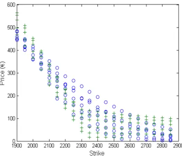
an estimation given by the user. The first naive attempt at running the optimization yielded the
results found in Figure 1 and Figure 2, for VG and GH processes respectively.
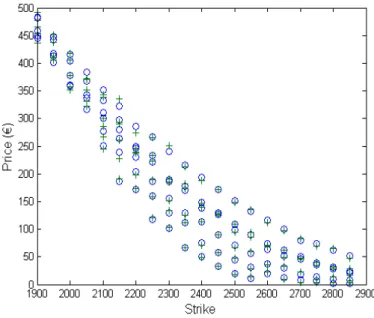
After running different initiations for the function, the results achieved improved substantially,
as can be seen in Figures 3 and 4. The modeled prices were nearer to the observed prices, and the
larger differences came from larger maturities or deep out-of-the-money options.
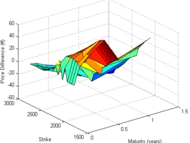
The surface of the differences between modeled prices and quoted prices are shown in Figure 5
and 6. The values for errors with VG have a higher range than the one with GH, which demonstrates
a better fit of the later model.
The highest difference was found in VG model: 13 euros, or 4% of the option value, as opposing
to Black-Scholes model results. Figure 7 shows the surface of discrepancies between BS prices and
observed prices. Here the errors are clearly larger than in the previous two models.
The calibration process might be improved with more robust computational tools.
Figure 1: First model calibration of VG distribution
Figure 2: First model calibration of GH distribution
estimation are presented on Figure 8.
5.2
Pricing exotic options
The options chosen to be priced were double barrier knock-out options, more precisely: a
Figure 3: Model calibration of VG distribution
Figure 4: Model calibration of GH distribution
money is just the sum of a put and a call at the same strike value K.
Let DB denote the down-and-out barrier and UB the up-and-out barrier of the options. The
strangle with a dual directional out barrier can be described as:
H =max(0, ST−K, K−ST)1DB<St<U B,0≤t≤T
Figure 5: Market prices minus modeled prices, via VG model
Figure 6: Market prices minus modeled prices, via GH model
It was not considered the forward start possibility. The pricing was performed on the 17th of
August, after close, considering the strike equal to Eurostoxx50 index closing value and the up and
down barriers were 130% and 70% of the strike, respectively.
We asked the price for this option to different possible counterparties, and priced it using Monte
Carlo simulation for both the VG and GH models as well as for the Black-Scholes assumptions.
Figure 7: Difference between Black-Scholes and market prices
Figure 8: Parameters estimation
the underlying price (jumps). Double barrier was used instead of single barrier because an analytic
closed formula is not known, only adaptations that require Laplace transformations calculations,
that are fast to compute and don’t require scenario simulation, such as Monte Carlo, but still
require convergence results for the calculations. So, the use of Monte Carlo can still be considered
adequate.
The results are presented below and are given in percentage, so we would not be dependent on
traded notional for these pricing. Indeed, over-the-counter quotes in percentage are very common:
Table 1: Prices for double knock-out option BS model VG model GH model Cntp. 1 Cntp. 2
Option Price 4.13% 7.26% 8.17% 8.47% 8.75%
As expected, the assumptions of BS applied to a Monte Carlo simulation to price this structure
It is referred in several articles that stochastic volatility modeling is becoming more and more
popular in the industry, and the prices that we received from market participants are likely to be
the result of such models. By using models with jumps we have obtained values that were closer
to market values. L´evy processes can also be used for stochastic volatility modeling, though this
6
Conclusions
In this thesis we assumed the price of an European index follows an exponential L´evy process,
and estimated the parameters for the Variance Gamma and Generalized Hyperbolic processes,
which are pure jump processes. When comparing the results of the estimated processes for vanilla
options pricing with the usual Black-Scholes model, we achieved better results. Results were better
overall, across maturities and strikes. It is worth noticing that the largest differences were observed
with deep out-of-the-money options, and higher maturities.
The exponential GH process evidenced a more stable approximation of the options market
surface. This was in line with our expectations, since the Variance Gamma is a special case of a
GH distribution. This fact enforces the idea that, though VG might be a clear improvement in
relation to a continuous diffusion model, the use of a more flexible process is justified.
Usually, other special cases such as the NIG or the Hyperbolic processes are estimated, but
one can generate the Generalized Hyperbolic by subordination of a Brownian motion with a GIG
process, enabling a structure that is not dependent on some pre-defined assumption for some of
the parameters.
The calibration to market prices consumes a lot of computational and numerical effort. The
work performed to calibrate the models showed the relevance of using strong estimation techniques,
as depending on predefined minimization toolboxes might yield an unsatisfactory calibration.
We used the calibrated models to price a double barrier option. This is a structure that is path
dependent and very sensitive to volatility. After analysing the prices with Monte Carlo simulation
for a diffusion model, both jump processes under study and the market prices for this derivative, we
found that the market prices were closer to the exponential L´evy models than to the exponential
Brownian motion.
After the completion of this work, some questions naturally arise. In the options surface there
were some discrepancies on out-of-the-money options, with longer maturities. One could study
whether the inclusion of stochastic volatility would diminish these differences considerably. Other
models could be studied as well, to test whether these differences would fade, like the CGMY or
Meixner processes. Additionally, posterior to an exotic option pricing, it could be tested whether a
hedging strategy supported by an exponential L´evy process would generate significant divergences
from the usual delta hedging supported by the Brownian motion.
Though superhedging is a possibility when considering hedging strategies, as it guarantees no
market, so further analysis in possible hedging strategies may be required for incomplete markets,
such as L´evy market models, as mentioned before. Besides, other tools such as fractional calculus
or Malliavin calculus might be required for dealing with more complex derivatives, or with barrier
options, where infinite derivatives might occur often, if the underlying approaches the barrier.
Stochastic volatility models may consider Brownian motion with a volatility parameter that
follows a stochastic process, may be a result of a subordination of a Brownian or L´evy process
by another L´evy process. A comparison between these models would be useful, since the effort
in calibrating these models depends on the type of process and the quantity of parameters to
be estimated, and the feasibility of the application will depend on this, so the gain of additional
7
Appendix A
DJ Eurostoxx50 Call Option Prices
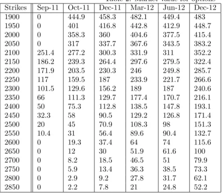
Listed below are 110 option prices on the DJ Eurostoxx50 index, at 13:05 of the 17th August, 2011. The index was at 2328.53. Estimated dividend yield for the next 12 months, according to Bloomberg data, was 5.10% and the interest rate for swaps on the euro, for maturity of 2 years, was 1.5341%.
Table 2: Market value for options Strikes Sep-11 Oct-11 Dec-11 Mar-12 Jun-12 Dec-12
1900 0 444.9 458.3 482.1 449.4 483
1950 0 401 416.8 442.8 412.9 448.7
2000 0 358.3 360 404.6 377.5 415.4
2050 0 317 337.7 367.6 343.5 383.2
2100 251.4 277.2 300.3 331.9 311 352.2
2150 186.2 239.3 264.4 297.6 279.5 322.4
2200 171.9 203.5 230.3 246 249.8 285.7
2250 117 159.5 187 233.9 221.7 266.6
2300 101.5 129.6 156.2 189 187 240.6
2350 66 111.3 129.7 177.4 170.7 216.1
2400 50 75.3 112.8 138.5 147.8 193.1
2450 32.3 58 90.5 129.2 126.8 171.4
2500 20 45 70.9 108.3 98 151.3
2550 10.4 31 56.4 89.6 90.4 132.7
2600 0 19.3 37.4 64 74 115.6
2650 0 12 30 51.9 61.6 100
2700 0 8.2 18.5 46.5 51 79.9
2750 0 5.9 13.4 36.3 38.5 73.3
2800 0 2.9 9.2 27.8 31.7 62.1
8
Appendix B
Matlab - most relevant code
function y = bs(x, r,q, sig, t)
d1 = (-log(x) + (r - q + 0.5 * sig2)∗t)/(sig∗sqrt(t));
d2 =d1−sig∗sqrt(t);
n1 =normcdf(d1);
n2 =normcdf(d2);
y= (exp(−q∗t)∗n1−x.∗n2∗exp(−r∗t));
function principal= VGcalibration(v0)
%Definition of the global variable
global OptPrice strike SpotsizeSsizeT lstrike pricesnorm r q a N eta b lambda alpha u x T B A;
%matrix of the prices of european call options
OptPrice = [0 444.9 458.3 482.1 449.4 483; 0 401 416.8 442.8 412.9 448.7; ...
0 358.3 360 404.6 377.5 415.4; 0 317 337.7 367.6 343.5 383.2; ...
251.4 277.2 300.3 331.9 311 352.2; 186.2 239.3 264.4 297.6 279.5 322.4; ...
171.9 203.5 230.3 246 249.8 285.7; 117 159.5 187 233.9 221.7 266.6;...
101.5 129.6 156.2 189 187 240.6; 66 111.3 129.7 177.4 170.7 216.1;...
50 75.3 112.8 138.5 147.8 193.1; 32.3 58 90.5 129.2 126.8 171.4;...
20 45 70.9 108.3 98 151.3; 10.4 31 56.4 89.6 90.4 132.7; 0 19.3 37.4 ...
64 74 115.6; 0 12 30 51.9 61.6 100; 0 8.2 18.5 46.5 51 79.9;
0 5.9 13.4 36.3 38.5 73.3; 0 2.9 9.2 27.8 31.7 62.1; 0 2.2 7.8 21 24.8 52.2];
%Strikes
strike= (1900:50:2850);
%Maturity of the considered options
T = [0.0806982 0.1765886 0.3300133 0.5793283 0.8286434 1.3464516];
Spot= 2328.53;
%parameters of the model
%risk free rate and dividend (annualized)
r = 0.01534;
q = 0.05109561;
%number of strikes and maturities for grid
sizeS = length(strike);
sizeT = length(T);
%log of the strike normalized by the spot
lstrike= log(strike/Spot);
%normalized matrix of prices
pricesnorm = OptPrice / Spot;
%integration grid - log strike grid
a = 600*2; % integration between 0 and a for the inverse Fourier transform
N = 4096*2; % strikes for FFT
A = zeros(sizeT, N);
B = zeros(sizeT, sizeS);
eta = a/N; % integration grid
b = pi/eta; % limits of the log-strike (-b,+b)
lambda = 2*pi/a; % step of the log strike
% Carr and Madan paramater (to avoid integration problem in 0) - 0.75 is
% suggested by Wim Schoutens in ”Levy Processes in Finance”
alpha = 0.75;
% integration grid
% log strike grid
x = -b + (0:N-1) * lambda;
f = @rootsqdif;
%Activate the following lines may improve precision for the minima search
options=optimset(’LargeScale’,’on’,’display’,’iter’,’TolFun’,1e-10,’TolX’,1e-10);
%search for the minima. The two vectors represent the range of the search
sigmam=f mincon(f, v0,[],[],[],[],[0.0050.0050.005],[151515],[], options);
maturF=[]; strikeF=[]; mktF=[]; calcul=[];
for j=1:sizeS
for l=1:sizeT
if OptPrice(j,l) ˜=0
strikeF = [strikeF, strike(j)];
marcheF = [mktF, OptPrice(j,l)];
calcul = [calcul , Spot*B(l,j)];
maturF = [maturF,T(l)];
end;
end;
end;
plot(strikeF,mktF,’o’,strikeF,calcul,’+’)
xlabel(’Strike’,’FontSize’,12)
ylabel(’Price ($)’,’FontSize’,12)
titre = ’Calibration: o market prices; + VG model’;
title(titre,’FontSize’,12,’FontWeight’, ’bold’)
print -dwin calibrationVG2011.eps
principal = sigmam;
Generalized hyperbolic generation:
%GH trajectories
function y = pathGH(Spot,r,q,x,alpha, beta, delta, lambda,n,deltat)
a =alpha2-beta2;
b =alpha2- (beta+ 1)2;
m = x*(r-q) + x * log((a/b)ˆ(lambda/2)*besselk(lambda,delta*sqrt(b))/besselk(lambda,delta*sqrt(a)));
%GIG number generator for the subordination
gig = GIGrn(delta2
t,lambda, alpha, beta,deltat, n);
Bm = normrnd(0,1,[1 n]);
% GH increments generation
deltax = Bm.*(gig.(1/2))+beta*gig;
v1 = zeros(1,n);
for i = 2:n;
v1(i)=v1(i-1)+deltax(i);
end;
%exponential of GH with drift to remain risk neutral
v2 = Spot*exp(v1).*(exp(m));
y = [max(v2), min(v2), v2(n)];
function z = GIGrn(lambda, a, b, delta, n)
gamma = sqrt(a2+b2);
beta = sqrt(gamma * delta);
m = (lambda-1 + sqrt((lambda−1)2+beta2)) / beta;
y1 = m;
y1= 2*y1;
while rootsg(y1,beta,m,lambda)<= 0
y1= 2*y1;
end;
y0 = m;
y2 = m;
y = y2;
y2 = 0.5 * (y0 +y1);
if rootsg(y2,beta,m,lambda) 0
y0=y2;
else
y1 = y2;
while abs(y2 - y)>= 0.00001*y2
y = y2;
y2 = 0.5 * (y0 +y1);
if rootsg(y2,beta,m,lambda) 0
y0=y2;
else
y1 = y2;
end;
end;
y0 = 0;
y1 = m;
y3 = 0;
y = y3;
y3 = 0.5 * (y0 + y1);
if rootsg(y3,beta,m,lambda) 0
y1 = y3;
else
y0 = y3;
end;
while abs(y3-y)>= 0.00001*y3
y = y3;
y3 = 0.5 * (y0 + y1);
if rootsg(y3, beta,m,lambda) 0
y1 = y3;
else
y0 = y3;
end;
end;
a1 = (y2 -m)*(y2/m)ˆ(0.5*(lambda-1))*exp(-0.25*beta*(y2+1/y2-m-1/m));
a2 = (y3 -m)*(y3/m)ˆ(0.5*(lambda-1))*exp(-0.25*beta*(y3+1/y3-m-1/m));
c = -0.25*beta*(m+1/m)+0.5*(lambda-1)*log(m);
value = zeros(1,n);
for i=1:n
r2 = unifrnd(0,1);
y = m + a1 * (r2/r1) + a2 * (1-r2)/r1;
while ˜(y ¿0 & -log(r1)¿=-0.5*(lambda-1)*log(y)+0.25*beta*(y+1/y)+c)
r1 = unifrnd(0,1);
r2 = unifrnd(0,1);
y = m + a1 * (r2/r1) + a2 * (1-r2)/r1;
end;
value(1,i) = y;
end;
References
Applebaum, D. (2009). L´evy Processes and Stochastic Calculus. Cambridge University Press.
Barndorff-Nielsen, O. E. (1977). Exponentially decreasing distributions for the logarithm of particle
size. Proceedings of the Royal Society of London, A353:pp. 401–419.
Bertoin, J. (1996). L´evy Processes. Cambridge University Press.
Bertoin, J. (1999). Subordinators: examples and applications. Ecole d’Et´e de Probabilit´es de St.
Flour XXVII, Lectures Notes in Mathematics 1717:4–79.
Carr, P. and Madan, D. (1998). Option valuation using the fast fourier transform. Journal of
Computational Finance, 2:pp. 61–73.
Cont, R. and Tankov, P. (2004).Financial Modelling With Jump Processes. Chapman & Hall/CRC.
Dagpunar, J. (1989). An easily implemented generalised inverse gaussian generator.
Communica-tions in Statistics - Simulation and Computation, 18:pp. 703–710.
Delbaen, F. and Schachermayer, W. (1998). The fundamental theorem of asset pricing for
un-bounded stochastic processes. Math. Ann., 312:pp. 215–250.
Dermoune, A. (1990). Distribution sur l’espaces de p. l´evy et calcul stochastique.Ann. Inst. Henri
Poincar´e, 26:pp. 101–119.
Eberlein, E. and Jacod, J. (1997). On the range of options prices. Finance Stoch., 1:pp. 131–140.
Eberlein, E. and Keller, U. (1995). Hyperbolic distributions in finance. Bernoulli, 1:pp. 281–299.
Eberlein, E. and Prause, K. (2001). The generalized hyperbolic model: financial derivatives and
risk measures. In: Mathematical Finance - Bachelier Congress 2000. H. Geman, D. Madan, S.
Pliska, and T. Vorst (eds.). Springer Verlag.
Eberlein, E., P. A. and Shiryaev, A. N. (2008). On the duality principle in option pricing:
semi-martingales setting. Finance Stoch., 12:pp. 265–292.
Geman, H. and An´e, T. (1996). Stochastic subordination. RISK, September.
Geman, H., M. D. and Yor, M. (2001). Time changes for l´evy processes. Math. Finance, 11:pp.
79–96.
Miyahara, Y. (1999). Minimal entropy martingale measures of jump type price processes in
in-complete asset markets. Asia-Pacific Financial Markets, 6:pp. 97–113.
Papapantoleon, A. (2008). An introduction to l´evy processes with applications in finance.
arXiv:0804.0482v2.
Prause, K. (1999).The Generalized Hyperbolic Model: Estimation, Financial Derivatives, and Risk
Measures. PhD thesis, University of Freiburg.
Protter, P. (1990). Stochastic integration and differential equations. Springer: Berlin.
Raible, S. (1998). L´evy processes in finance: theory, numerics and empirical facts. PhD thesis,
University of Freiburg.
Sato, K. (1999).L´evy Processes and Infinitely Divisible Distributions. Cambridge University Press.
Schoutens, W. (2003). L´evy Processes in Finance: Pricing Financial Derivatives. John Wiley &
Sons, Inc.