Inflation and business cycle convergence in the euro area: empirical analysis using an unobserved component model

Inflation and Business Cycle Convergence in the Euro

Area: Empirical Analysis Using an Unobserved

Component Model

Abstract The literature on optimum currency areas states that large inflation differentials can undermine monetary union. In the euro area, inflation rates diverged after the creation of the single currency, but started to converge again from mid-2002. Against this background, we assess the convergence of inflation rates and business cycles and study the relationship between them. The analysis is made using an unobserved component model estimated with the Kalman filter. In general, from 1980 to 2008 inflation rates and business cycles became more aligned in the euro area, but inflation rates converged more quickly than business cycles. The output gap is found to be a better indicator of the business cycle than unit labour cost when studying convergence. By looking at the causality between the convergence of inflation and output gap, it is found that inflation divergence has a limited destabilising economic impact.

Keywords Inflation convergence

.

.

.

JEL Classifications E31

.

1 Introduction

As stressed by the optimum currency area literature, large inflation differentials can undermine the success of a monetary union (Tavlas 1994). Moreover, since the business cycle is one of the main drivers of inflation, there should be a relationship between convergence of inflation rates and convergence of business cycles. The main goal of this paper is to study the association between these two convergence processes, namely we want to examine whether divergence (convergence) in inflation rates after the

S. G. Hall

University of Leicester, Leicester, UK e-mail: [email protected] S. Lagoa (*)

Instituto Universitário de Lisboa–ISCTE, Avenida das Forças Armadas, 1649-026 Lisboa, Portugal e-mail: [email protected]

S.G. Hall, S. Lagoa

introduction of the euro can be explained by divergence (convergence) in business cycles.

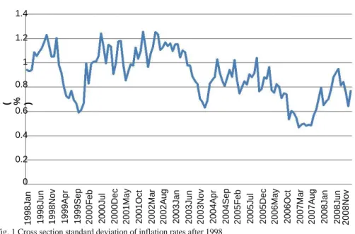
Since the creation of the European Exchange Rate Mechanism (ERM) in 1979, there has been evidence that monetary policy convergence in the euro area has been accompanied by inflation convergence. However, inflation divergence was observed after the introduction of the euro (Lane 2006; Busetti et al. 2007), as can be seen in Fig. 1. Due to the nominal convergence required by the Maastricht Criteria, the cross-sectional standard deviation of inflation rates in the euro area decreased to 0.6 % in September 1999. 1 This was followed by a rise until it reached 1.2 % in mid-2002. The downward trend in inflation dispersion started again after this peak, falling to the lowest level ever of 0.47 % in March 2007. In the first years of the euro (1999–2002), the countries with highest inflation rates were Greece, Ireland, the Netherlands, Portugal and Spain.

We can point several reasons for the initial increase in inflation differentials after the launch of the euro. Firstly, inflation divergence may be due to equilibrating mecha-nisms as long-run relative price levels across countries depend on relative productivity and income levels. Therefore, since economic and monetary integration may lead to convergence of productivity and income, the poor countries will have temporarily higher inflation rates. This is the Balassa-Samuelson effect, which is more important in the long-run. Inflation differentials can also replace nominal exchange rate adjust-ments since countries with low inflation gain external competitiveness (Lane 2006).

A further explanation for inflation differentials relies on the fact that the baskets of goods and services used to measure CPI inflation differ from country to country. However, these differences have not been of much importance since the creation of the euro (ECB 2003; Honohan and Lane 2003).

The euro may also produce inflation differentials with destabilizing macroeconomic consequences. The nominal convergence between countries before the creation of the euro meant a bigger decline in real interest rates in peripheral countries. This implied a faster growth of credit, house prices, aggregate demand, and therefore inflation for those countries. This one-off expansionary shock dissipated over time as higher inflation led to the real appreciation of the currency.

Temporary asymmetric shocks are recurrent in a monetary union; positive demand shocks in which short-run supply rigidities create transitory inflation are an example of this. Without a national monetary policy, the ability to deal with these shocks is limited as inflation differentials cannot be corrected by currency depreciation in high-inflation countries. In the case of deflationary shocks, countries may use expansionary fiscal policy to solve the problem, but this can lead to a violation of the Stability and Growth Pact with negative effects on the financial markets in the euro area (Honohan and Lane 2003).

The ability to deal with asymmetric shocks will be even more limited if shocks are persistent. When the labour market is not flexible, with current rather than future inflation determining wage growth, higher inflation today may lead to higher wage growth thus triggering an upward spiral of wage growth and inflation. Indeed, Vines et al. ( 2006) show that when inflation is expressively persistent, countries in a monetary union may be subject to large and long cycles in GDP after asymmetric shocks. In their

1

Inflation and Business Cycle Convergence in the Euro Area 1.4 1.2

Fig. 1 Cross section standard deviation of inflation rates after 1998

model, fiscal policy can play an important part in reducing inflation differences between countries.

In addition, in a monetary union, higher than average inflation rates produce lower than average real interest rates; this may lead to both excessive debt accumulation and a rise in property prices, followed by a painful adjustment process. The differences in business cycles among countries can then be exacerbated, widening inflation differen-tials even further in a cycle of divergence (Honohan and Lane 2003; Dullien and Fritshe 2008).

However, there are two empirically relevant stabilising mechanisms in the euro area (Hofmann and Remsperger 2005). Firstly, GDP growth in one country has positive output spillover effects on other countries, which contributes to the reduction of inflation differentials. Naturally, this mechanism is more relevant for large countries due to the limited impact of small countries on others. Secondly, the real exchange rate acts as a correcting mechanism: countries with higher than average inflation rates, will face a real appreciation that reduces demand and inflationary pressures. Even though this correction occurs gradually, the effect accumulates over time since external competitiveness depends on relative price levels.

Following our literature review of inflation and business cycle dynamics in a monetary union, we now highlight the most innovative features of this paper and our contribution to the literature. The analysis of the convergence of business cycles using the Kalman filter, as proposed by Hall et al. ( 1997), is new in the literature. In addition, the literature on convergence has largely ignored the real Unit Labour Cost (ULC) as an indicator of the business cycle despite its importance in the New Keynesian approach to inflation. 2 In addition, the joint analysis of the convergence of inflation and business cycles with Hall et al. ( 1997)’s model has two novelties. First, we compare the rates at 2

In the New Keynesian Phillips Curve the driver of inflation is the marginal cost, which can be measured using the labour income share, also called real unit labour cost.

S.G. Hall, S. Lagoa

which the (unobserved) convergence of inflation and business cycles evolves over time. Second, we analyse the two-way causality between inflation and business cycles convergence.

Our results indicate that inflation differentials in the euro area converged in expec-tation from 1980 to 2008. However, there was some temporary divergence after the creation of the euro, especially in Greece, Ireland, the Netherlands, Portugal and Spain. The business cycles of euro area countries also became more aligned; this is more evident when using the output gap than the real or nominal ULC. A further finding is that inflation rates converged faster than output gaps. When looking at the causality between these two variables, on one hand, output gap divergence is likely to cause cumulative inflation divergence, and on the other hand, a cumulative inflation diver-gence tends to lead to business cycle converdiver-gence.

The remainder of the paper is organised as follows. In Section 2 the main concepts of convergence are revised. Next, in Section 3 we analyse the convergence of inflation over the period 1980–2008, using the Kalman filter to test whether the variance of the unobserved convergence component decreased over time. In Section 4 we apply the same methodology to study the convergence of business cycles. The rates of conver-gence of inflation and output gap are compared in Section 5 before studying the causality between them in Section 6. Finally, Section 7 concludes.

2 The Methodology for Measuring Convergence

There are several ways of measuring economic convergence and there is no consensus as to the best method. Hall et al. ( 1997) refer to three definitions of convergence: point wise, in expectation and in probability. The most appealing definition is convergence in expectation, which occurs when the limit of the expected value of the scaled difference between two series (Xt and Yt for instance) converges to a constant:

lim E ð X _t−θY _t Þ ¼ α t→∞

This definition allows the difference between the two series to be random in the limit. This is an adequate feature to measure the convergence of economic time series because they are usually measured with error, and thus the variance of their difference will not go to zero asymptotically, as demanded by the concept of convergence in probability.

It is easy to see that if two series are stationary, then they converge in expectation. However, the discussion of convergence typically occurs in the context of non-stationary series, where we have at least three situations. Firstly, if the difference zt = Xt

−θYt is non-stationary as t goes to infinity, then there is no convergence by any of the

previous definitions, since the variance of zt will not go to zero asymptotically and there

is no long-run mean to which series converge. Secondly, if Xt and Yt are non-stationary

but cointegrated (and the cointegration residuals are I(0)), then they have converged in expectation but not necessarily in probability. Many studies have used the concept of cointegration between series and the stationarity of the difference of two series to assess inflation convergence (for example Holmes 2002; Busetti et al. 2007; Gregoriou et al. 2007). Thirdly, it is possible that two series are non-stationary and non-cointegrated for

Inflation and Business Cycle Convergence in the Euro Area

the entire sample, but they convergence at the end of the sample. This occurs when the difference between variables becomes stationary after an initial period of non-stationary behaviour due to changes in the economic environment. This means that cointegration is not a necessary condition for convergence. As Hall et al. ( 1997) highlight, convergence is defined as a limiting case, while cointegration is a concept that applies to the entire sample.

On the other hand, Hall et al. ( 1997) propose a more appealing way to measure convergence that makes use of time-varying parameters and allows convergence to take place gradually as the series generating process evolves towards stationarity. Therefore, this methodology deals adequately with structural breaks in convergence processes. The proposed model is then:

where εt is a random error that accounts for measurement errors. The model’s central

element is the unobserved component αt, which measures the convergence between

series, and depends on an error term vt, with initial variance given by Ω0. If the variance

of vt converges to zero (f <1), then αt will evolve to a non-stochastic constant, and

convergence in expectation is guaranteed. A formal test involves the null hypothesis of non-convergence H₀ :f=1. If the null is rejected in favour of the alternative hypothesis f <1 and the variance of εt is zero, then convergence in probability also occurs. This

framework encompasses the evaluation of convergence based on cointegration. In fact, an estimate of Ω0=0 for I(1) series means that they are cointegrated.

Notice that this model is in the state-space form, with Eq. ( 1) as the measurement or observation equation and Eq. ( 2) as the state or transition equation. The Kalman filter must be applied to the state-space form equations, where αt is the

state variable. Firstly, this filter provides “optimal” forecasts of the unobserved component αt. 3 Then, these forecasts are used to generate series of one-step-ahead

prediction errors and their variances, which contain unknown parameters to be estimated. Finally, using these series of errors and variances, standard maximum likelihood techniques can be used to estimate the unknown parameters.

The described model decomposes the difference between two series in two compo-nents: a permanent component, αt, which we interpret as a measure of convergence, and

an error εt, which is a transitory component. What the Kalman filter actually does is to

determine which part of the change in the dependent variable, Xt −θYt, can be attributed

to each of these components.

We can also use a similar model to test for each country if output gap and inflation converge at the same rate:

dif xit ¼ α x t þ ε x t ð3Þ 3

S.G. Hall, S. Lagoa i π π (4) dif πt¼ αt þ εt αtx ¼ αtx−1 þ vtx; αtπ ¼ αtπ−1 þ vtπ; εtx∼N 0; σx2 ; εtπ∼N 0; σπ2 ; vtx∼N 0; Ωtx ; vtπ∼N 0; Ωtπ ; Ωtπ ¼ fΩtπ−1; Ω0π given; Ωtx ¼ ffzΩtx−1; Ω0 x ¼ Ω0πΩ0z given;

where dif xit =xit −xeurot, with xit being the output gap of country i and xeurot the output gap

of the euro area. Also dif πit =πit −πeurot, with πit as the inflation rate of country i and πeurot

as the inflation rate of euro area. Equations ( 3) and ( 4) are estimated simultaneously. Since the convergence rates of the variances of unobserved components (and also the initial variances) are allowed to be different for inflation and output gap, these convergence rates can be compared. If we do not reject H0:f

z

=1, the two convergence processes occur at the same rate, Ωt/Ωt−1 =f . These processes will be even more similar if the initial variances of the

state variables also coincide, i.e., if we do not reject H0:Ωz0=1.

After looking at the first extension of Hall et al. ( 1997)’s model, we can turn to the second extension to assess the two-way causality between the convergence processes of inflation and business cycle, using the state variable αt as the convergence indicator. To

study this, two changes have been made to the model comprising Eqs. ( 3) and ( 4). First, we assume that the last period’s state variable of the output gap may affect the current state variable of inflation (Eq. ( 8) below). And since causality can be bidirectional, it was also assumed that the last period’s state variable of inflation may influence the current state variable of output gap (Eq. ( 7) below). This leads to the following model, where all equations are estimated simultaneously for each country i:

dif xt i ¼ αt x þ εt x ð5Þ dif πt i ¼ αtπ þ εtπ ð6Þ αt x ¼ γggαt x −1 þ γigαtπ−1 þ vt x ð7Þ αtπ ¼ γiiαtπ−1 þ γgiαtx−1 þ vtπ (8) εtx∼N 0; σx2 ; εtπ∼N 0; σπ2 ; vtx∼N 0; Ωtx ; v_tπ∼N 0; Ωtπ ; Ωt x ¼ fxΩt x −1; Ω0 x given; Ωtπ ¼ fπΩtπ−1; Ω0π given:

Some comments are necessary regarding the γ parameters. Firstly, we allowed γgg and γii

to be different from one to ensure the model’s stability. Moreover, when one of the series converges and the other does not, only some values for γ make sense. If the output gap converges but inflation does not, then γig=0. Otherwise, in the limit there was a

non-stationary component in the output gap. Likewise, if the output gap does not converges but inflation does, we should have γgi=0. Finally, if both series converge, γig and γgi may or may

not be different from zero. In the next sections, we apply the above models to the convergence of inflation and business cycles in the euro area.

Inflation and Business Cycle Convergence in the Euro Area

3 Convergence of Inflation Rates

In this section we study inflation convergence from 1980 to 2008. A relatively large period is analysed to put the evolution of inflation rates during the euro period in a historical context. The focus is on the convergence of each country towards the euro average, analysing the difference between each country’s inflation rate and the euro average: πi,t-πeur,t, where πi,t is the inflation rate of country i in period t, and

πeur,t is the euro area inflation rate. 4

When available, we used the quarterly harmonised CPI from Eurostat after removing seasonality; otherwise the non-harmonised CPI from OECD Main Economic Indicators was used. For the euro area seasonally adjusted data was obtained from ECB.

Our goal is to see whether inflation differences evolve gradually towards stationarity, as outlined in the model composed by Eqs. ( 1) and ( 2). Under the null hypothesis f=1, model (1) is non-stationary and f is in the boundary of the likelihood space. 5 Therefore, under the null the test statistic follows a non-standard distribution. Using Monte Carlo simulations, Hall et al. ( 1997) suggest that f is asymptotically normally distributed and that standard errors are underestimated by a factor that varies between 1.65 and 2.0. 6

Looking at Table 1, the null of non-convergence is not rejected only for Austria, Germany and the Netherlands. In the former two cases the z-statistics is higher than 1.8, but in the latter case it is smaller than one indicating a clear non-rejection of the null. The reason for this may be related with the fact that there is not a clear reduction in inflation’s volatility for these three countries, unlike for the others (Fig. 2). Indeed, inflation rates of these countries were already more stable at the beginning of the sample and their average inflation differentials were among the lowest. In addition, the null hypothesis that the variance of the state variable was zero in the first period or in the last period for each of the three countries is not rejected (fifth and sixth columns of Table 1, respectively). In other words, these countries already had a very high degree of convergence in 1980Q1, and hence the test does not identifies further convergence afterwards. In addition, notice that the variance of the state variable in 2008Q4 converged to zero for the other countries as well (sixth column of Table

1). In summary, there is evidence of inflation convergence in the euro area in the period 1980–2008.

However, the above statement does not mean that sub-periods of divergence did not exist. In fact, Becker and Hall ( 2009) show that inflation co-movement was smaller after the creation of the euro than before. Such divergence can be identified in our approach, for each country, when the unobserved convergence variable, αt, is

signif-icantly different from zero. An estimate of that variable can be obtained using its filtered value, and the root mean squared error (RMSE) can be used to assess whether that estimate is statistically different from zero. 7

4

πi,t: quarterly inflation rate annualised: (1 + inf quarterlyt)4−1, where inf quarterlyt=pt/p_t−1−1, with p as the CPI.

5

Note that with f >1 the model is explosive.

6

Consequently, the z-statistics critical value at 5 % significance for rejecting the null hypothesis (using a one-sided test: H₀:f=1 vs H₀:f<1) should be (in absolute value) between 2.71 (=1.65*1.645) and 3.29 (=2*1.645). 7

The filtered value of αt is computed as follows. Firstly, the one-step ahead forecast for period t is obtained using information until t-1. The filtered state of αt corresponds to the update of this forecast using information up to t.

S.G. Hall, S. Lagoa Table 1 Measuring inflation convergence towards euro area with time-varying parameters

Var(εt) f f−1 Ω80Q1 Ω08Q4 α09Q1|08Q4

Austria

Coeff. 8E-05*** 0.8900* −0.1099 0.0008 1.31E-09 −0.0026**

s.e./RMSE 1.13E-05 0.0392 0.0006 5.8E-09 0.0012

z stat. 7.0796 −2.8035 1.4151 0.2258 −2.0921

Log likelih. 340.23 Belgium

Coeff. 0.0001*** 0.9274** −0.0725 9.74E-05** 1.69E-08 0.0005

s.e./RMSE 1.2E-05 0.0193 5.74E-05 3.56E-08 0.0016

z stat. 8.3333 −3.7533 1.6968 0.4747 0.3448

Log likelih. 339.2969 France

Coeff. 4.08E-05*** 0.8858*** −0.0662 0.0012** 1.09E-09 −0.0026***

s.e./RMSE 6.69E-06 0.0235 0.0006 2.96E-09 0.0009

z stat. 6.0986 −4.8485 2.0261 0.3682 −2.6805

Log likelih. 367.1511 Finland

Coeff. 0.0001*** 0.9634*** −0.0365 0.0002** 3.8E-06 0.0041

s.e./RMSE 2.75E-05 0.0075 0.0001 3.08E-06 0.0051

z stat. 5.2727 −4.8358 2.2080 1.2337 0.7929

Log likelih. 300.1584 Germany

Coeff. 7.16E-05*** 0.9613 −0.0386 9.18E-05 9.9E-07 −0.0024

s.e./RMSE 8.31E-06 0.0207 8.8E-05 1.58E-07 0.0030

z stat. 8.6161 −1.8623 1.0431 0.6265 −0.7852

Log likelih. 346.3500 Greece

Coeff. 0.0001*** 0.9388*** −0.0611 0.0141** 1E-05 0.0092

s.e./RMSE 2.78E-05 0.0098 0.0061 8.26E-06 0.0062

z stat. 3.5971 −6.2280 2.3100 1.2106 1.4918

Log likelih. 237.7761 Ireland

Coeff. 0.0001*** 0.9204*** −0.0795 0.0058*** 4.25E-07 0.0038

s.e./RMSE 2.69E-05 0.0084 0.0014 3.96E-07 0.0032

z stat. 4.9814 −9.4265 3.9276 1.0732 1.2050

Log likelih. 275.9299 Italy

Coeff. 7.09E-05*** 0.9191*** −0.0808 0.0010*** 6.33E-08 0.0024

s.e./RMSE 1.11E-05 0.0100 0.0003 6.52E-08 0.0018

Inflation and Business Cycle Convergence in the Euro Area Table 1 (continued)

Var(εt) f f−1 Ω80Q1 Ω08Q4 α09Q1|08Q4

Luxembourg

Coeff. 0.0001*** 0.9173*** −0.0826 0.0005 2.64E-08 0.0053**

s.e./RMSE 2.75E-05 0.0185 0.0004 4.93E-08 0.0021

z stat. 6.0000 −4.4478 1.2321 0.5354 2.4823

Log likelih. 304.3132 Netherlands

Coeff. 0.0001*** 1.0095 0.0095 9.01E-06 2.68E-05 0.0012

s.e./RMSE 2E-05 0.0156 1.07E-05 2.3E-05 0.0084

z stat. 5.9000 0.6084 0.8420 1.1652 0.1520

Log likelih. 321.8492 Portugal

Coeff. 0.0001*** 0.9167*** −0.0833 0.0169*** 7.7E-07 0.0005

s.e./RMSE 4.2E-05 0.0112 0.0060 8.73E-07 0.0039

z stat. 4.3333 −7.4375 2.8095 0.8820 0.1333

Log likelih. 244.1434 Spain

Coeff. 0.0001*** 0.9030** −0.0969 0.0019 1.59E-08 0.0098***

s.e./RMSE 2.8E-05 0.0274 0.0013 4.55E-08 0.0019

z stat. 5.0000 −3.5373 1.4433 0.3494 4.9433

Log likelih. 301.7576

Estimation with the Kalman Filter, 1980Q1–2008Q4

The z-statistics are for the null of each respective coefficient equal to zero, except for f where the null is f =1. ***–Reject the null at 1 % significance level, **–at 5 %, and *–at 10 %. The significance refers to one-sided tests, except for α09Q1|08Q4 where it refers to two-sided test. For the significance of the null hypothesis f =1 see footnote 6. For the final one-step ahead values of the state variable, we present the corresponding RMSE

From Fig. 2 and Table 2, an increase can be observed in positive divergence (in the sense that the state variable stays significantly above zero for a certain number of periods) in some quarters after 1998 for Greece, Ireland, Italy, Luxembourg, the Netherlands, Portugal and Spain. In line with this finding, Busetti et al. ( 2007) identify Portugal, Greece, Ireland and Spain as a group where inflation differentials were stable after 1998, but with higher than average inflation rates. Notice that the divergence for these countries may have been associated with the significant reduction in the real interest rate that accompanied the nominal convergence to the euro.

In contrast, for Austria, Finland, France and Germany there are periods of negative divergence with the euro average. But for all countries, except Austria, France, Luxembourg and Spain, the divergence is reversed at the end of the sample. For these four countries, the indicator of convergence (the final filtered value of the state variable αt) is statistically different from zero in the last period of the sample (seventh column of

S.G. Hall, S. Lagoa Austria Belgium .04 .02 .02 .01 .00 .00 -.01 -.02 -.02 -.03 -.04 -.04 -.06 -.05 -.06 -.08 -.07 82 84868890 92 949698 0002 04 0608 82 848688 909294 9698000204 0608 Finland France .06 .06 .04 .04 .02 .02 .00 .00 -.02 -.02 -.04 -.04 -.06 -.06 82 848688 9092 94 9698 00 0204 0608 82 848688 909294 9698000204 0608 Germany Greece .04 .35 .02 .30 .25 .00 .20 -.02 .15 -.04 .10 .05 -.06 .00 -.08 -.05 82848688909294969800 020406 08 82848688 9092949698000204 0608 Ireland Italy .20 .14 .12 .15 .10 .10 .08 .06 .05 .04 .00 .02 .00 -.05 -.02 82 8486889092 94969800 0204 0608 82 848688 9092949698000204 0608 Luxembourg Netherlands .06 .06 .04 .04 .02 .02 .00 .00 -.02 -.02 -.04 -.04 -.06 -.06 -.08 -.08 82 8486889092 94969800 0204 0608 8284 8688 90 92 94 96 98 00 0204 0608 Portugal Spain .4 .12 .3 .10 .08 .2 .06 .1 .04 .02 .0 .00 -.1 -.02 82 84 86 88 90 92 94 96 9800 0204 0608 82848688 90 92 94 96 98 00 02040608

Fig. 2 Inflation differentials towards EA, filtered state variable, 1980Q1–2008Q4. Note: these graphs represent the filtered state variable and the upper and lower limit of the 95 % significance interval

Inflation and Business Cycle Convergence in the Euro Area

and France, it is positive for Luxembourg and Spain. In addition, the indicator of divergence for Luxembourg is half that of Spain, and the divergence occurred for a shorter period. This suggest that this situation had only a significant negative impact on the external competitiveness of Spain. In con-clusion, inflation divergence in general was temporary in nature.

4 Convergence of Business Cycles

Given that there is a strong relationship between business cycles and inflation, our hypothesis is that inflation convergence in the euro area has been accom-panied by convergence in business cycles. While output gap has traditionally been the preferred measure of business cycles, the New Keynesian approach argues that the real Unit Labour Cost (ULC) is the correct driver of inflation. Given this disagreement, we will use these two indicators, beginning with the real ULC.

4.1 Convergence of Real ULC

The literature has devoted some attention to wages and productivity as determinants of inflation divergence. For example, the ECB Inflation Persistence Network concluded that the most important source of inflation differentials in the euro area was the “sustainable differential in wage growth and narrower differences in productivity growth” (ECB 2003).

In this paper, we analyse the convergence of wages and productivity by looking at real ULC. This variable has the advantage of combining wages (w_t) and labour

Table 2 Quarters of statistically significant divergence in inflation after the creation of the euro Country Average of the state variable No. of quarters Quarters of divergence

in the diverging period of divergence

Austria −0.3626 26 1999Q2–Q3, 2002Q1, 2003Q1–2004Q4, 2005Q2–2008Q4 Finland −1.3792 11 2004Q1–2006Q3 France −0.3395 39 1999Q1–2004Q3, 2005Q1–2008Q4 Germany −0.8477 8 2002Q2–2004Q1 Greece 1.7277 11 2000Q4, 2001Q3–2002Q4, 2003Q2, 2005Q1, 2006Q3–Q4 Ireland 1.8260 25 1999Q3–2005Q1, 2006Q4–2007Q1 Italy 0.6662 7 1999Q1–1999Q3, 2000Q1–Q2, 2003Q2, 2003Q4 Luxembourg 0.5869 14 2005Q3–2008Q4 Netherlands 2.0184 8 1999Q1, 2001Q1–2002Q3 Portugal 1.5478 12 1999Q1, 2001Q1–2003Q3 Spain 1.0407 40 1999Q1–2008Q4

S.G. Hall, S. Lagoa

productivity (pr_t). In fact, real ULC (s_t) can be written in logs as: s_t =ulc_t −pd_t =w_t −pr_t − pd_t, where ulc_t is the nominal ULC and pd_t the GDP deflator. Notice that nominal ULC is given by w_t −pr_t.

There is some previous work by Dullien and Fritshe ( 2008) on the convergence of growth rates of nominal ULCs in the EMU using annual data between 1960 and 2007. These authors do not reject the hypothesis of convergence for all EMU countries on two grounds. Firstly, nominal ULC growth differentials towards the average are stationary. Secondly, there is cointegration between ULC growth rates of individual countries and the rest of the EMU. There is also no evidence of a structural break in the convergence of nominal ULC growth rates caused by the introduction of the euro.

Using a Panel Analysis of Nonstationarity in the Idiosyncratic and Common com-ponents (PANIC), Fritsche and Kuzin ( 2007) are more pessimistic regarding nominal ULC growth convergence in the euro area. They found that it is difficult to identify a common factor, with idiosyncratic factors explaining the majority of the variance. Moreover, countries respond to the common factor in very different ways, and it is possible to identify two groups of countries. One is the “hard currency” club, composed of Austria, Belgium, Germany, Luxembourg and the Netherlands. The other group includes Finland, Greece, Ireland, Portugal and Spain, which have common move-ments due to their catching-up processes.

Contrary to Fritsche and Kuzin ( 2007) and Dullien and Fritshe ( 2008), we prefer the real ULC to the nominal ULC because it is the correct driver of inflation in the New Keynesian Phillips Curve. Our initial focus is on the convergence tests applied to the difference between the log of real ULC of each country and the euro average. The real ULC was obtained by dividing the nominal ULC by the GDP deflator, with both indexes with base 100 in 2005. The seasonally adjusted nominal ULC for the entire economy and the seasonally adjusted GDP deflator were both obtained from the OECD.

8

Since data are expressed in indices, convergence is not expected towards the same level of real ULC. Nevertheless, if two countries converge, we expect to observe their real ULCs moving together, implying that real ULCs differential fluctuate around a constant (not necessarily zero). However, it is possible that at the beginning of the convergence process the co-movement of real ULC between a high inflation country and euro area will be small. A high inflation country aiming to reduce inflation rate to the euro area level must go through an initial period of strong reduction in real ULC. This will naturally imply an initial divergence between the two series. But once inflation has converged, it is expected that real ULCs will basically grow at the same rate in both countries. This justifies the use of the unobserved convergence component approach based on the Kalman filter, which is able to detect on-going convergence.

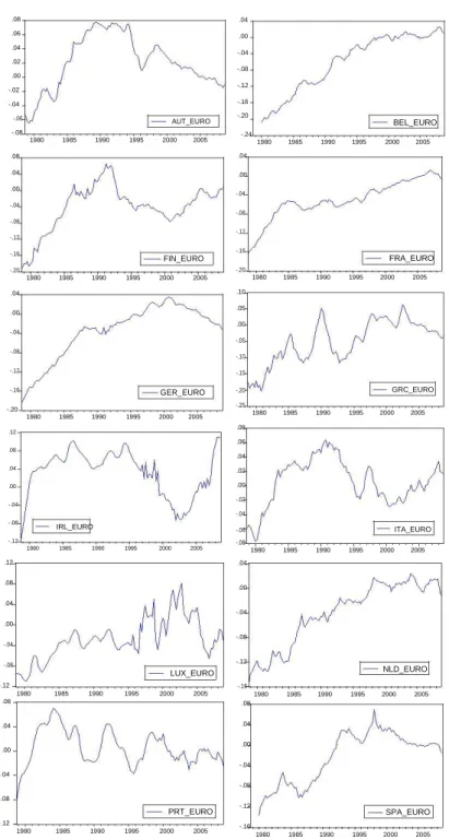
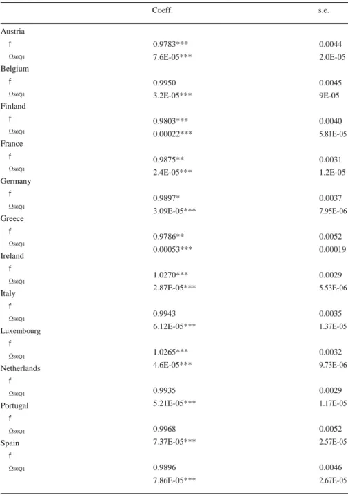
The graphs of real ULC differentials do not show a clear pattern of convergence (Fig. 3). Confirming this, the formal test shows convergence at 5 % significance only for Austria, Finland, France and Greece (Table 3).

We can observe from the graphs of the real ULC of the four countries for which the test identified convergence that the convergence process is not yet

8

The nominal ULC series excludes also the irregular movements in the underlying series. Moreover, since the ULC of the entire economy was not available for Portugal, we used the ULC of the business sector.

Inflation and Business Cycle Convergence in the Euro Area .08 .06 .04 .02 .00 -.02 -.04 -.06 AUT_EURO -.08 1980 1985 1990 1995 2000 2005 .08 .04 .00 -.04 -.08 -.12 -.16 FIN_EURO -.20 1980 1985 1990 1995 2000 2005 .04 .00 -.04 -.08 -.12 -.16 _{GER_EURO} -.20 1980 1985 1990 1995 2000 2005 .12 .08 .04 .00 -.04 -.08 IRL_EURO -.12 1980 1985 1990 1995 2000 2005 .12 .08 .04 .00 -.04 -.08 LUX_EURO -.12 1980 1985 1990 1995 2000 2005 .08 .04 .00 -.04 -.08 PRT_EURO -.12 1980 1985 1990 1995 2000 2005 .04 .00 -.04 -.08 -.12 -.16 -.20 BEL_EURO -.24 1980 1985 1990 1995 2000 2005 .04 .00 -.04 -.08 -.12 -.16 FRA_EURO -.20 1980 1985 1990 1995 2000 2005 .10 .05 .00 -.05 -.10 -.15 -.20 GRC_EURO -.25 1980 1985 1990 1995 2000 2005 .08 .06 .04 .02 .00 -.02 -.04 -.06 ITA_EURO -.08 1980 1985 1990 1995 2000 2005 .04 .00 -.04 -.08 -.12 NLD_EURO -.16 1980 1985 1990 1995 2000 2005 .08 .04 .00 -.04 -.08 -.12 SPA_EURO -.16 1980 1985 1990 1995 2000 2005

Fig. 3 Log difference between the real ULC of each country and the euro area. Note: X_EURO: the log difference between the real ULC of country X and the average of the euro area. Country headings: AUT– Austria, BEL–Belgium, FIN–Finland, FRA–France, GER–Germany, GRC–Greece, IRL– Ireland, ITA–Italy, LUX–Luxembourg, NLD–The Netherlands, PRT–Portugal, and SPA–Spain

S.G. Hall, S. Lagoa Table 3 Measuring real ULC convergence towards euro area with time-varying parameters

Coeff. s.e. Austria f Ω80Q1 Belgium f Ω80Q1 Finland f Ω80Q1 France f Ω80Q1 Germany f Ω80Q1 Greece f Ω80Q1 Ireland f Ω80Q1 Italy f Ω80Q1 Luxembourg f Ω80Q1 Netherlands f Ω80Q1 Portugal f Ω80Q1 Spain f Ω80Q1 0.9783*** 0.0044 7.6E-05*** 2.0E-05 0.9950 0.0045 3.2E-05*** 9E-05 0.9803*** 0.0040 0.00022*** 5.81E-05 0.9875** 0.0031 2.4E-05*** 1.2E-05 0.9897* 0.0037 3.09E-05*** 7.95E-06 0.9786** 0.0052 0.00053*** 0.00019 1.0270*** 0.0029 2.87E-05*** 5.53E-06 0.9943 0.0035 6.12E-05*** 1.37E-05 1.0265*** 0.0032 4.6E-05*** 9.73E-06 0.9935 0.0029 5.21E-05*** 1.17E-05 0.9968 0.0052 7.37E-05*** 2.57E-05 0.9896 0.0046 7.86E-05*** 2.67E-05

Estimation with the Kalman Filter, 1980Q1–2008Q4

The z-statistics are for the null hypothesis f=1 or Ω1980Q1 =0. ***–Reject the null at 1 % significance level, **–at 5 %, and *–at 10 %. The significance refers to one-sided tests. For the significance of the null hypothesis

f=1 see footnote 6. Initially, we assumed Var(εt)≠0, but this variance was not significantly different from zero.

Inflation and Business Cycle Convergence in the Euro Area

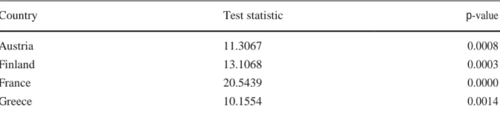
Table 4 Testing whether the variance of the convergence variable for the real ULC is zero in 2008Q4

Country Test statistic p-value

Austria 11.3067 0.0008

Finland 13.1068 0.0003

France 20.5439 0.0000

Greece 10.1554 0.0014

Wald test with the null hypothesis H0 :Ω2008Q4 =0 is performed for the countries for which convergence

was obtained in Table 3. The test statistics has a Chi-square distribution under the null

finished. To formally confirm this, a Wald test will be performed to analyse if the variance of the state variable, var(v_t), is zero in the last quarter of the

sample: H₀ : Ω2008Q4 =0. 9 For the four countries where convergence was detected,

this test rejects the null, confirming the incompleteness of the

convergence process (Table 4). In fact, the variance of the state variable residual was decreasing, but had not yet reached zero in 2008Q4. This means that the real ULC differentials still have a non-stationary behaviour with convergence in expectation not yet achieved, but in the limit the variance will go to zero.

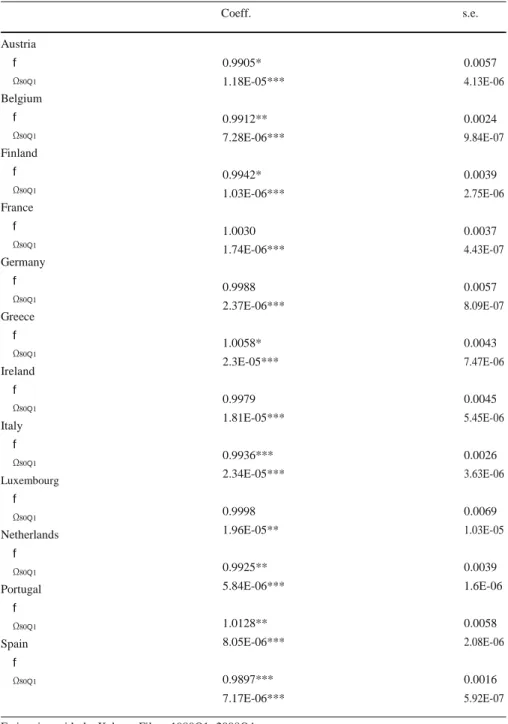
Since there is weak evidence of real ULC convergence, we next analyse the convergence of nominal ULC growth. Our results show convergence (at 5 % level of significance) only for Belgium, Italy, the Netherlands and Spain (Table 5). 10 This supports the results of Fritsche and Kuzin ( 2007).

In conclusion, convergence in inflation was achieved despite a rather incomplete convergence of real and nominal ULC. This casts doubts over the ability of both real and nominal ULC to explain inflation convergence. Therefore, in the next section we analyse output gap convergence, expecting to find better evidence of business cycles convergence.

4.2 Convergence of Output Gaps

In this section, we study the convergence of output gaps in the euro area by analysing the difference between the output gap of each country and the euro area output gap. This indicator measures the synchronisation of business cycles, but the variance is not expected to go exactly to zero, because output gap is measured with some error. Instead, it is sensible to assume that as business cycles become more synchronised,

9

Regarding this test, it is worth noting that as a Wald test is asymptotically equivalent to a likelihood ratio test, the null hypothesis tests more than whether the variance is zero in the last period. In fact, it tests whether a full path of convergence exists, leading to a zero variance in the last period.

10

Notice that for the growth rates of the nominal ULC we are not interested in studying if there is convergence in expectation, because that is already ensured as these variables are stationary. Instead, our main goal is to understand how the variance of these variables evolves over time. As a result, we can use the standard critical value 1.675 for a one-sided test at 5 % significance.

S.G. Hall, S. Lagoa

Table 5 Measuring nominal ULC growth convergence towards euro area with time-varying parameters

Austria f Ω80Q1 Belgium f Ω80Q1 Finland f Ω80Q1 France f Ω80Q1 Germany f Ω80Q1 Greece f Ω80Q1 Ireland f Ω80Q1 Italy f Ω80Q1 Luxembourg f Ω80Q1 Netherlands f Ω80Q1 Portugal f Ω80Q1 Spain f Ω80Q1 Coeff. s.e. 0.9905* 0.0057 1.18E-05*** 4.13E-06 0.9912** 0.0024 7.28E-06*** 9.84E-07 0.9942* 0.0039 1.03E-06*** 2.75E-06 1.0030 0.0037 1.74E-06*** 4.43E-07 0.9988 0.0057 2.37E-06*** 8.09E-07 1.0058* 0.0043 2.3E-05*** 7.47E-06 0.9979 0.0045 1.81E-05*** 5.45E-06 0.9936*** 0.0026 2.34E-05*** 3.63E-06 0.9998 0.0069 1.96E-05** 1.03E-05 0.9925** 0.0039 5.84E-06*** 1.6E-06 1.0128** 0.0058 8.05E-06*** 2.08E-06 0.9897*** 0.0016 7.17E-06*** 5.92E-07

Estimation with the Kalman Filter, 1980Q1–2008Q4

The z-statistics are for the null hypothesis f=1 or Ω1980Q1 =0. ***–Reject the null at 1 % significance level, **–at 5 %, and *–at 10 %. The significance refers to one-sided tests. For the significance of the null hypothesis

f=1 we used standard critical values. Initially, we assumed Var(εt)≠0, but this variance was not significantly different

Inflation and Business Cycle Convergence in the Euro Area

the variance of the difference between output gaps decreases. 11 The various studies on the evolution of output gap correlation in the euro area have not reached an unanimous conclusion (De Haan et al. 2008). Our analysis will assess whether there is convergence/divergence of output gaps, for the full period, despite possible short periods of convergence/divergence.

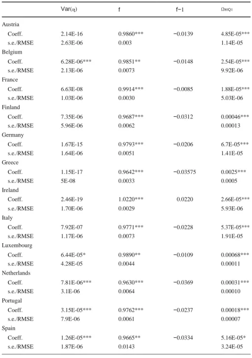
The output gap was obtained as the difference between the log of output and the log of the trend output. To obtain the trend output we used the Hodrick-Prescott filter, with lambda fixed at 1600. The real GDP data was obtained from the OECD for all countries except Portugal, for which IMF data is used. Applying the methodology to the data shows that the variance of output gap differentials for all countries except Ireland decreased in a statistically significant way between 1980 and 2008 (Table 6). 12 Notice that the result for Ireland is strongly affected by the steep decline in output gap that occurred in 2008.

The convergence of business cycles in the euro area was probably explained by the deepening of trade and monetary integration. In particular, the adoption of a system of fixed exchange rates in 1979 and the subsequent creation of a single currency implied convergence of policies that may have led to greater conformity in business cycles. Artis and Zhang ( 1997, 1999) defend that a similar evolution occurred when the European ERM was created.

The convergence rates vary from −1.09 % per quarter for Luxembourg to −3.69 % per quarter for the Netherlands (Table 6). 13 In addition, some interesting patterns can be identified. On one hand, there is a group of countries with smaller rates of convergence: Austria, Belgium, France and Luxembourg. It is probable that the output gap of these countries was already highly synchronised with the euro area in 1980. On the other hand, we have the Southern countries: Greece, Italy, Portugal and Spain. These countries, which were less linked to the euro area business cycle in 1980, converged at higher rates. In addition, Finland, which had strong trade links with the former Soviet Union, had a quick convergence towards the euro area business cycle.

In general, business cycles of euro area countries became more aligned from 1980, probably due to the increasing economic and monetary integration.

5 Comparing the Convergence Processes of Inflation and Output Gap

We see from the above that there is strong evidence of convergence in inflation rates and robust evidence of convergence of output gaps. In this context, it would be interesting to know if both processes occurred at the same rate. To answer this question, we estimated the model composed of Eqs. ( 3) and ( 4).

For Finland and Germany the convergence processes of inflation and output gap occurred at the same rate, since we do not reject H0 :f

z

=1 (Table 7). 14 For Ireland and the Netherlands we did not make the test because the non-convergence hypothesis was 11

Once more, we are not interested in studying if there is convergence in expectation because that is already ensured as output gaps are stationary variables.

12

In this test we use the standard critical values to test H0: f=1, because the difference of output gaps is

stationary even if H0 is not rejected. 13

The convergence rate is Ωt/Ωt−1 −1=f−1.

14

S.G. Hall, S. Lagoa Table 6 Measuring output gap convergence towards euro area with time-varying parameters

Var(εt) f f−1 Ω80Q1

Austria

Coeff. 2.14E-16 0.9860*** −0.0139 4.85E-05***

s.e./RMSE 2.63E-06 0.003 1.14E-05

Belgium

Coeff. 6.28E-06*** 0.9851** −0.0148 2.54E-05***

s.e./RMSE 2.13E-06 0.0073 9.92E-06

France

Coeff. 6.63E-08 0.9914*** −0.0085 1.88E-05***

s.e./RMSE 1.03E-06 0.0030 5.03E-06

Finland

Coeff. 7.35E-06 0.9687*** −0.0312 0.00046***

s.e./RMSE 5.96E-06 0.0062 0.00013

Germany

Coeff. 1.67E-15 0.9793*** −0.0206 6.7E-05***

s.e./RMSE 1.64E-06 0.0051 1.41E-05

Greece

Coeff. 1.15E-17 0.9642*** −0.03575 0.0025***

s.e./RMSE 5E-08 0.0033 0.0005

Ireland

Coeff. 2.46E-19 1.0220*** 0.0220 2.66E-05***

s.e./RMSE 1.70E-06 0.0029 5.93E-06

Italy

Coeff. 7.92E-07 0.9771*** −0.0228 5.37E-05***

s.e./RMSE 1.17E-06 0.0073 1.91E-05

Luxembourg Coeff. 6.44E-05* 0.9890** −0.0109 0.00068*** s.e./RMSE 4.28E-05 0.0044 0.00011 Netherlands Coeff. 7.81E-06*** 0.9630*** −0.0369 0.00031*** s.e./RMSE 3.1E-06 0.0064 0.00010 Portugal Coeff. 3.15E-05*** 0.9762*** −0.0237 0.00018*** s.e./RMSE 7.9E-06 0.0061 0.00007 Spain

Coeff. 1.26E-05*** 0.9665** −0.0334 5.16E-05*

s.e./RMSE 1.87E-06 0.0143 3.24E-05

Estimation with the Kalman Filter, 1980Q1–2008Q4

The z-statistics are for the null of each respective coefficient equal to zero, except for f where the null is f=1.

***–Reject the null at 1 % significance level, **–at 5 %, and *–at 10 %. The significance refers to one-sided tests. Standard critical values were used for the test regarding f

Inflation and Business Cycle Convergence in the Euro Area

Table 7 Testing the equality of the convergence processes of inflation and output gap

Coeff. s.e. Austria fz Ωz80Q1 (1−fπ)−(1−fx) Belgium fz Ωz80Q1 (1−fπ)−(1−fx) Finland fz Ωz80Q1 (1−fπ)−(1−fx) France fz Ωz80Q1 (1−fπ)−(1−fx) Germany fz Ωz80Q1 (1−fπ)−(1−fx) Greece fz Ωz80Q1 (1−fπ)−(1−fx) Italy fz Ωz80Q1 (1−fπ)−(1−fx) Luxembourg fz Ωz80Q1 (1−fπ)−(1−fx) Portugal fz Ωz80Q1 (1−fπ)−(1−fx) Spain fz Ωz80Q1 (1−fπ)−(1−fx) 1.1099** 0.0481 0.0534*** 0.0445 −0.0976 1.0649*** 0.0204 0.2146*** 0.1515 −0.0619 1.0031 0.0222 1.1307 0.6312 −0.0030 1.120*** 0.027 0.013*** 0.007 −0.106 1.0148 0.017 0.812 0.687 −0.0143 1.0271*** 0.0119 0.1848*** 0.1007 −0.025 1.064*** 0.0126 0.047*** 0.022 −0.059 1.077*** 0.022 1.272 1.056 −0.071 1.068*** 0.014 0.010*** 0.0053 −0.062 1.077** 0.0323 0.018*** 0.018 −0.070 Estimation with the Kalman Filter, 1980Q1–2008Q4

These coefficients result from the estimation of the unobserved component model composed of (3) and (4). To save space, only two coefficients are presented. The z-statistics are for the null of each coefficient equal to one.***–Reject the null at 1 % significance level, **–at 5 %, and *–at 10 %. Significance levels are for two-sided tests and based on standard critical values

S.G. Hall, S. Lagoa

not rejected for one of the variables in a very clear manner. For the remaining eight countries, the processes were distinct, with the convergence of inflation occurring at a faster rate than the convergence of the output gap: on average 6.9 % per quarter faster. The same occurs for Finland and Germany, but the difference in the convergence dynamics of the two variables was not statistically significant. The reason for a faster convergence of inflation than output gap may be found in the Maastricht criteria that stressed the importance of nominal convergence.

It is worth mentioning that the comparison between the rates of convergence of inflation and output gap does not elucidate about the causality between the two phenomena. For instance, the two processes may have occurred at the same rate because other factors implied a common rate of convergence. Therefore, in the next section we study the causality between the two processes of convergence.

6 Causality Between the Convergence of Inflation and Output Gap

There are many reasons why the convergence of inflation and the convergence of output gap may influence each other. For easier understanding, in what follows we refer to divergence that is simply the reverse of convergence. On one hand, when a country’s output gap is higher than the average output gap, there is pressure for its inflation to be also higher than average. On the other hand, divergence of inflation may affect that of the output gap even though the direction of the impact is unclear. It is true that when a country’s inflation is growing faster than average, this leads to a loss of competitiveness, which cools down the economy and brings about convergence of output gap. On the other hand, high inflation leads to lower real interest rates, which increases aggregate demand and output gap divergence. We must use empirical means to determine which of these effects is dominant.

Some papers have already linked output gap and inflation differentials. Using annual data, Rogers ( 2002), Honohan and Lane ( 2003), Honohan and Lane ( 2004) and Angeloni and Ehrmann ( 2007) conclude for the significance of output gap in explaining inflation differences in the euro area. However, when Honohan and Lane ( 2004) uses quarterly data concludes for the insignificance of output gap. Our work contributes to this literature by estimating with quarterly data a new model to assess convergence–the unobserved component model composed of (5) and (6)–which allows a two-way causality between inflation and the business cycle.

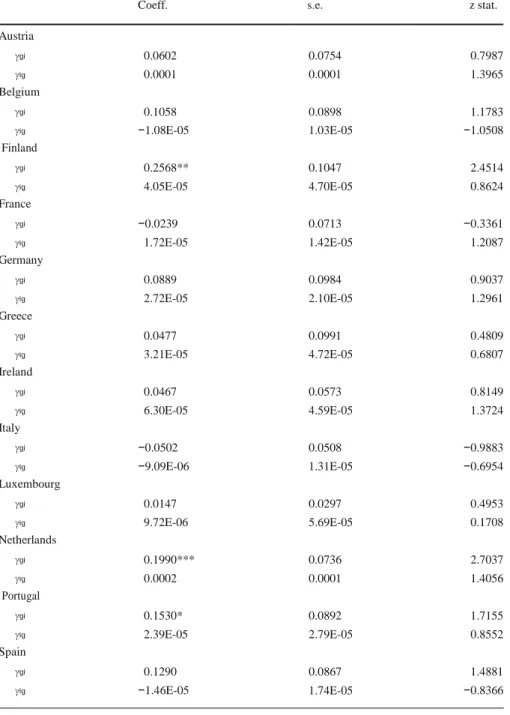
As expected from the discussion above, our results (Table 8) show that the effect of output gap divergence on inflation divergence is positive for all countries except for France and Italy, but is never statistically significant except for Finland, the Netherlands and Portugal (the latter at 10 % significance level). On the other hand, the sign of the effect of inflation divergence on output gap divergence is positive, except for Belgium, Italy and Spain, but it is never statistically significant.

So far, our evidence shows that the causality between the two processes is statisti-cally weak. However, it is well known that the impact of inflation differentials has a cumulative effect on the cyclical position, because price differences undermine the external competitive position in a permanent way. Therefore, we next analyse the cumulative effect of inflation divergence on output gap divergence. To that end, we

Inflation and Business Cycle Convergence in the Euro Area Table 8 Causality between convergence of inflation and output gap

Coeff. s.e. z stat.

Austria γgi 0.0602 0.0754 0.7987 γig 0.0001 0.0001 1.3965 Belgium γgi 0.1058 0.0898 1.1783 γig −1.08E-05 1.03E-05 −1.0508 Finland γgi 0.2568** 0.1047 2.4514 γig 4.05E-05 4.70E-05 0.8624 France γgi −0.0239 0.0713 −0.3361 γig 1.72E-05 1.42E-05 1.2087 Germany γgi 0.0889 0.0984 0.9037 γig 2.72E-05 2.10E-05 1.2961 Greece γgi 0.0477 0.0991 0.4809 γig 3.21E-05 4.72E-05 0.6807 Ireland γgi 0.0467 0.0573 0.8149 γig 6.30E-05 4.59E-05 1.3724 Italy γgi −0.0502 0.0508 −0.9883 γig −9.09E-06 1.31E-05 −0.6954 Luxembourg γgi 0.0147 0.0297 0.4953 γig 9.72E-06 5.69E-05 0.1708 Netherlands γgi 0.1990*** 0.0736 2.7037 γig 0.0002 0.0001 1.4056 Portugal γgi 0.1530* 0.0892 1.7155 γig 2.39E-05 2.79E-05 0.8552 Spain γgi 0.1290 0.0867 1.4881 γig −1.46E-05 1.74E-05 −0.8366

Estimation with the Kalman Filter, 1980Q1–2008Q4

These coefficients result from the estimation of the unobserved component model composed of (5) and (6). To save space, only two coefficients are presented. The z-statistics are for the null of each individual coefficient equal to zero. ***–Reject the null at 1 % significance level, **–at 5 %, and *–at 10 %. Significance levels are for two-sided tests and based on standard critical values

S.G. Hall, S. Lagoa Table 9 Causality between convergence of CPI and output gap

Coeff. s.e. z stat.

Austria γgi 0.0900* 0.0491 1.8297 γig −0.0009*** 2.60E-05 −34.6175 Belgium γgi 0.0360 0.0684 0.5261 γig 0.0009*** 2.09E-06 463.4060 Finland γgi 0.0746*** 0.0206 3.6224 γig −0.0162*** 0.0007 −20.5568 France γgi 0.0263*** 0.0019 13.3666 γig 0.0015 0.0017 0.9002 Germany γgi 0.1015* 0.0581 1.7467 γig 0.0010 0.0029 0.3539 Greece γgi 0.0006 0.0473 0.0143 γig 2.72E-05 0.0031 0.0085 Ireland γgi 0.0078*** 7.71E-05 102.1373 γig −0.0108 0.0079 −1.3620 Italy γgi 0.0125 0.0620 0.2018 γig −0.0010*** 0.0001 −6.1782 Luxembourg γgi 0.0106 0.0136 0.7825 γig 0.0010 0.0489 0.0210 Netherlands γgi 0.1421** 0.0557 2.5480 γig −0.0101*** 0.0010 −9.8890 Portugal γgi 0.1530* 0.0892 1.7155 γig 2.39E-05 2.79E-05 0.8552 Spain γgi −0.0056 0.0680 −0.0824 γig −0.0016 0.0033 −0.4852

Estimation with the Kalman Filter, 1980Q1–2008Q4

These coefficients result from the estimation of the unobserved component model composed of (5) and (6) using the difference of CPIs instead of the difference of inflation rates. To save space, only two coefficients are presented. The z-statistics are for the null of each individual coefficient equal to zero.***–Reject the null at 1 % significance level, **–at 5 %, and *–at 10 %. Significance levels are for two-sided tests and based on standard critical values

Inflation and Business Cycle Convergence in the Euro Area

use the percentage difference of CPIs instead of the difference of inflation rates and we obtain more significant results than previously (Table 9). An increase in the distance of output gap from the euro average increases CPIs differentials for all countries (except Spain), and this relation is statistically significant for Austria, Finland, France, Germany, Ireland, Netherlands and Portugal. 15

Reverse causality also exists: when CPI is above the euro average, output gap differences tend to decrease, and this relationship is statistically significant for Austria, Finland, Italy and the Netherlands. For Ireland and Spain, the effect is also negative but not statistically significant. Belgium is the only country for which CPI divergence has a positive and statistically significant effect on output gap divergence. For France, Germany, Greece, Luxembourg and Portugal that effect is also positive but not statistically significant. One explanation for the non-statistical significance of this effect for some countries may be that the two effects of inflation divergence on output gap divergence described above tend to compensate each other. In sum, these results show that inflation differentials tend to have a non-statistically significant effect on output gap divergence or tend to reduce it, which limits the destabilising effects of inflation differentials.

7 Conclusion

This paper addresses two major issues: assessing the convergence of inflation rates and business cycles in the euro area, and studying the relationship between these conver-gence processes. We started by analysing the convergence of inflation, real ULC, nominal ULC and output gap towards the euro average. From 1980 to 2008, inflation differentials in the euro area converged in expectation, despite the emergence of some temporary divergence after the introduction of the euro. This transitory diverging dynamic was more significant for Greece, Ireland, the Netherlands, Portugal and Spain.

Business cycles of euro area countries also became more aligned between 1980 and 2008, and this was clearer when they were measured using the output gap. Together with the above evidence on inflation, this indicates that the output gap is a better indicator of business cycle than the real or nominal ULC when studying inflation convergence.

For countries where convergence of output gap and inflation was identified, conver-gence of inflation occurred at a faster rate than that of output gap. When examining the causality between the two phenomena, an increase in output gap divergence leads to cumulative divergence in inflation for a considerable number of countries. In the opposite direction, a cumulative increase in inflation divergence tends to reduce business cycles divergence. As a result, the destabilising impact of inflation divergence is limited.

Our results allow making some comments on the recent developments in the euro area. Inflation divergence observed in Greece, Ireland, Italy, Portugal, and Spain was responsible for the reduction in economic growth that contributed to the 2010 Sovereign Debt Crisis. Because of this crisis, business cycle divergence of these countries from the rest of the euro area deepens. This causes divergence in terms of

15

S.G. Hall, S. Lagoa

inflation; while this helps these countries to regain external competitiveness, it may make it more difficult to resolve the private and public debt problems. In the long run, a more sustainable euro area depends on the deepening of economic and monetary integration, supported by strong fiscal and monetary policies at the European level, leading to an alignment of business cycles and inflation rates.

Acknowledgments We are grateful to Kevin Lee, Simon Wren-Lewis, the anonymous referees and George S. Tavlas (the Editor-in-Chief) for helpful comments and suggestions. The usual disclaimer applies. Sérgio Lagoa thanks the financial support of Fundação para a Ciência e Tecnologia, scholarship SFRH/BD/27973/2006. References

Angeloni I, Ehrmann M (2007) Euro area inflation differentials. BE J Macroecon 7:1

Artis MJ, Zhang W (1997) International business cycles and the ERM: is there a European Business cycle? Int J Financ Econ 2:1–16

Artis MJ, Zhang W (1999) Further evidence on the international business cycle and the ERM: is there a European business cycle? Oxf Econ Pap 51:120–132

Becker B, Hall S (2009) A new look at economic convergence in Europe: a common factor approach. Int J Financ Econ 14:85–97

Busetti F, Forni L, Harvey A, Venditti F (2007) Inflation convergence and divergence within the European Monetary Union. Int J Cent Bank 3(2):95–121

De Haan J, Inklaar R, Jong-A-Pin R (2008) Will business cycles in the Euro area converge? A critical survey of empirical research. J Econ Surv 22(2):234–273

Dullien S, Fritshe U (2008) Does the dispersion of unit labor cost dynamics in the EMU imply long-run divergence? IEEP 5:269–295

ECB (2003) Inflation differentials in the Euro Area: potential causes and policy implications. ECB Report, Frankfurt, September

Fritsche U, Kuzin V (2007) “Unit labor growth differentials in the Euro area, Germany, and the US: lessons from PANIC and cluster analysis.” German Institute for Economic Research DIW Discussion Paper No. 667, Berlin, February

Gregoriou A, Kontonikas A, Montagnoli A (2007) “Euro area inflation differentials: unit roots, structural breaks and non-linear adjustment.” Department of Economics University of Glasgow Working Paper No. 13/2007, Glasgow, June

Hall SG, Robertson D, Wickens MR (1997) Measuring economic convergence. Int J Financ Econ 2:131–143 Hofmann B, Remsperger H (2005) Inflation differentials among the Euro area countries: potential causes and

consequences. J Asian Econ 16:403–419

Holmes MJ (2002) Panel data evidence on inflation convergence in the European Union. Appl Econ Lett 9: 155–158

Honohan P, Lane PR (2003) Divergent inflation rates in EMU. Econ Policy 18:357–394

Honohan P, Lane PR (2004) "Exchange Rates and Inflation Under EMU: An Update," CEPR Discussion Papers 4583, London, August

Lane PR (2006) The real effects of European Monetary Union. J Econ Perspect 20:47–66

Rogers JH (2002) “Monetary union, price level convergence, and inflation: how close is Europe to the United States?.” International Finance Discussion Papers No. 740, Board of Governors of the Federal Reserve System. Washington, DC, October

Tavlas GS (1994) The theory of monetary integration. Open Econ Rev 5:211–230

Vines D, Kirsanova T, Wren-Lewis S (2006) Fiscal Policy and Macroeconomic Stability within a Currency Union, CEPR Discussion Paper No. 5584, London, March