REM WORKING PAPER SERIES
Investors' Perspective on Portfolio Insurance
Expected Utility vs Prospect Theories
Raquel M. Gaspar and Paulo M. Silva
REM Working Paper 092-2019
September 2019
REM – Research in Economics and Mathematics
Rua Miguel Lúpi 20,
1249-078 Lisboa,
Portugal
ISSN 2184-108X
Any opinions expressed are those of the authors and not those of REM. Short, up to
two paragraphs can be cited provided that full credit is given to the authors.
Expected Utility vs Prospect Theories
Raquel M. Gaspar · Paulo M. Silva
September 2019
Abstract This study supports the use of behavioural finance to explain the popularity of portfolio insur-ance. Portfolio insurance strategies are important financial solutions sold to institutional and individual investors, that protect against downside risk while maintaining some upside valuation potential. The way some of these strategies are engineered has been criticised, and portfolio insurance itself blamed for increasing market volatility in depressed markets. Despite this, investors keep on buying portfolio insurance that has a solid market share. This study contributes to understand the phenomenon.
We compare investors’ decision using two distinct frameworks: expected utility theory and behavioural theories. Based upon Monte Carlo simulation techniques we compare portfolio insurance strategies against uninsured basic benchmark strategies.
We conclude that cumulative prospect theory may be a viable framework to explain the popularity of portfolio insurance. However, among portfolio insurance strategies, na¨ıve strategies seem to be preferable to most commonly traded strategies.
Keywords portfolio insurance · expected utility · prospect theory · Monte Carlo simulation JEL Classification: G11, G13, G17
1 Introduction
Portfolio insurance (PI) strategies have been a popular investment alternative for institutional and retail investors since the 1980’s. Despite its designation, a PI strategy is not an insurance contract, where an investor pays a premium for a risk transference to an insurance company to limit losses from adverse market conditions. Instead, it is a dynamic asset allocation strategy.
The two most common PI strategies are option–based portfolio insurance (OBPI) and constant pro-portion portfolio insurance (CPPI). The OBPI was developed after the seminal article of Black and Scholes (1973), when Leland and Rubinstein (1976) suggested the use of options for hedging portfolios. About a decade later, Perold (1986) and Black and Jones (1987) proposed CPPIs.
From an incumbent market in the late 70s and early 80s, PI investments gained momentum, and became important in the asset management industry. Due to falling costs on trading, and exuberant product innovation (e.g. structured financial products, index notes, warrants, etc.), PI have also expanded from institutional solutions to retail investments, suggested to individual investors.
ISEG – REM
Rua Miguel Lupi 20, room 510 1200-781 Lisboa, Portugal E-mail: Rmgaspar@iseg.ulisboa.pt ISEG – CGS and Lusitania
Financial markets, specially since de 1980s, have suffered several crises impacting investors’ wealth. The intensity of those crises varied across markets and asset classes, but the uncertainty became a permanent factor in investors’ decisions. This environment of uncertain outcomes, coupled with global integration, and the increasing complexity of investment alternatives, drove investors’ decisions into a more demanding risk management process, also explaining why market players kept on developing and proposing PI strategies to provide both hedging and leverage solutions.
Ironically, since the Brady (1988) report, PI strategies have been identified as possibly responsible for the increasing severity of financial market crisis. On this matter, important references are Shiller (1988), Dybvig (1988), Brennan and Schwartz (1989), Rubinstein (1999), Tucker (2005), Leland (2011), Vandenbroucke (2015) and Bertrand and Prigent (2016). In spite of this, the fact is that PI investments remain attractive to both institutional and retail investors – see, for instance Pain and Rand (2008) and Vrecko and Branger (2009).
The current importance of PI is clear when in November 11th 2015, The New York Times dedicates its wealth special section to the subject describing the most recently developed strategies (Wasik 2015) or when Forbes, in March 4th 2016, recommends its usage after the strong equity returns on 2016 and the rising fear of losses on the increasing wealth from market returns (Russell 2016). With the opposite view on PI, the Financial Times March 21st 2017 claims that the rise of new forms of portfolio insurance spark fears (Wigglesworth 2017), at The Wall Street Journal October 19th 2017, the Nobel prize winner Prof. Robert Shilller notes that there is a resurgent idea about PI as a solution that was designed to protect investors from falling markets but, instead, it could lead to a new market panic as in 1987 (Shiller 2017) and Bloomberg Opinion in October 25th 2017 calls for caution (Gandel 2017).
When taking the investors’ perspective, several studies have also questioned the optimality of PI strategies. Using the von Neumann and Morgenstern (1947) classical expected utility theory (EUT) we have, among others, Benninga and Blume (1985), Black and Perold (1992), Cesari and Cremonini (2003), Annaert, Van Osselaer, and Verstraete (2009), or Bertrand and Prigent (2016). Black and Perold (1992), for instance, documented that a CPPI strategy, with unconstrained borrowing, only maximizes expected utility when investors show hyperbolic absolute risk aversion utility functions. More importantly, Vrecko and Branger (2009) show that averse investors would not choose PI investments over unhedged alternatives, such as a plain investment in the risky asset.
EUT and the traditional finance paradigm considers agents to be rational, i.e. it assumes that when agents receive new information, they update their beliefs correctly, and that given their beliefs, they make choices that are normatively acceptable. This traditional framework is appealingly simple, and it would be very satisfying if its predictions were empirically confirmed. However, after years of effort, it has become clear that basic facts about the aggregate stock market, the cross-section of average returns and individual trading behaviour are not easily understood in this framework (see Samuelson (1977)). Behavioural theories of Tversky and Kahneman (1974), Kahneman and Tversky (1979) and Tversky and Kahneman (1992) has emerged in response to these difficulties, arguing that investors are not fully rational. In fact, experimental results show investors tend to be more averse to losses than gains, which seem aligned with the PI downside protection profile. See Barberis and Thaler (2003) for an overview on behavioural issues. Vrecko and Branger (2009) and Dichtl and Drobetz (2011) were the first to look at PI investments from a behavioural perspective. More recent related studies are Bernard and Kwak (2016), Deng and Liu (2017), Silva (2018), and Escobar, Lichtenstern, and Zagst (2019).
This paper is in line with that latest stream of literature that considers the investor viewpoint. It uses Monte Carlo simulations to compare PI strategies, and plain investments on stock market and the riskless asset, to find how capable are the previously mentioned alternative theories – the traditional EUT, and behavioural prospect and cumulative prospect theories (PT and CPT) – of explaining the persistent popularity of portfolio insurance. It reproduces some results in the existing literature, but represents a more exhaustive study by considering not only popular PI strategies and non-PI investments, but also na¨ıve PI strategies. With respect to the na¨ıve strategies, it considers the safety–first strategy first introduced by Costa and Gaspar (2014), that turns out to be the dominant PI strategy in almost all scenarios, even when behavioural theories are considered.
The remaining of the text is organised as follows: Section 2 defines the framework for portfolio insurance and sets the notation. The methodology and simulation features are set in Section 3. Section 4 presents and discusses the results. Finally, Section 5 concludes summarising the main results and discussing future research.
2 Portfolio Insurance
Portfolio insurance (PI) is a term that characterises investment strategies, which offer an investor the ability to limit the downside risk, and, simultaneously, to keep the possibility of benefiting from the upside potential of an underlying risk asset or portfolio.
Overall PI can be understood as a distributor of financial risk among agents willing to absorb it. In fact, issuers of portfolio insurance solutions can be exposed to relevant downside risk (unexpected high losses), enhancing the conditions to more volatile financial markets.
Despite the concerns from the literature, and the increasing complexity of risk management decisions, PI popularity has not decreased. If some PI strategies became controversial and lost popularity (e.g. CPPIs, see discussion in Carvalho, Gaspar, and Sousa (2016)), other have emerged in their place. Pain and Rand (2008) summarises some of the developments until then, from which we highlight various mod-ifications of the original CPPI strategy: from the Time Invariant Portfolio Protection (TIPP) proposed by Estep and Kritzman (1988), to the “cushion insurance” of Prigent and Tahar (2005), the dynamics proportions proposed by Chen, Chang, Hou, and Lin (2008) or the contingent retracted floor of Lee, Hsieh, and Hsu (2013). Hocquard, Papageorgiou, and Remillard (2015) proposes alternative strategies with pre-specified distributional properties that present much better results than CPPIs and Bernard and Kwak (2016) suggests modifications taking the perspective of the pension funds industry and long-term investors.
Nowadays investors are, thus, presented with a wide range of strategies, offered from very active distribution channels on retail banking and institutional segments.
This section briefly presents the PI strategies under analysis and presents a brief literature review.
2.1 Portfolio Insurance Strategies
The implementation of portfolio insurance is possible both using PI strategies commonly traded in the market, and na¨ıve strategies that can be directly implemented by investors, as they require no financial engineering.
Historically, the most popular PI strategies on retail and institutional markets are the synthetic Option-Based Portfolio Insurance (OBPI) and the Constant Proportion Portfolio Insurance (CPPI) with a multiplier superior to 1. As plain CPPIs lost popularity, Time Invariant Portfolio Protection (TIPP) became also very popular (amongst the array of variants from plain CPPIs).
On the na¨ıve side, we have the classical Stop Loss Portfolio Insurance (SLPI) and the more recently suggested safety-first strategy, which turn out to be nothing but a CPPI with a multiplier equal to 1 (CPPI1).
Table 1 summarises the PI strategies under analysis.
Table 1 List of major portfolio insurance strategies
Portfolio Insurance Strategies Na¨ıve strategies Complex strategies
SLPI
CPPI CPPI TIPP OBPI
m = 1 m > 1 Dynamic Floor
Synthetic Options
Stop Loss Portfolio Insurance (SLPI)
In a SLPI strategy, the investor sets the equivalent to a stop loss order, which is a conditional instruction to sell the risky underlying if it’s value falls below a given level – floor. In this case, an investor, who allocates the total initial wealth (V0) in the underlying risky asset, cuts the loss to the
major problem with this strategy is its path dependency (Rubinstein (1985)): when market falls below the predefined floor portfolio, stock is sold and converted into cash/bonds, which are then held until maturity. From that moment on, there is independence on future market movements until maturity.
The investor position in the risky underlying is held as long as the present value of the floor (Ft) is
smaller than the current wealth (portfolio value at time t), i.e. the investor will be 100% invested in the risky underlying as long as Vt> Ft) and it will be 100% invested in the risk free asset otherwise. Thus
the exposure to risky underlying (ESt):
ESt=
(
Vt, if Vt> Ft
0, if Vt≤ Ft,
(1)
where the value of the floor at maturity FT = K is the guaranteed amount.
If the market value of the risky underlying falls below the floor Ft, the portfolio is sold and converted
into the risk-free asset and held until maturity. EBtdenotes the strategy’s exposure to the riskless asset.
Therefore, at maturity, the value of a SLPI stratgey (VSLP I), is given by:
VTSLP I = EST + EBT
(
EST = 0 ∧ EBT = ESter(T −t), if Vt< Ft,
EST = WT ∧ EBT = 0, if Vt≥ Ft.
(2)
Option-Based Portfolio Insurance(OBPI)
Investors, pursuing an OBPI strategy, mimic a portfolio investing in the risky asset, the riskless asset and at-the-money options on the risky asset. OBPIs can be understood as a static strategy, when it happens that the option can be bought, but that is rarely feasible for the desired maturities, strikes or underlying (see Lee, Finnerty, Lee, Lee, and Wort (2013)). In practice, the option component is dynamically synthesised using only the risky and riskless asset, as proposed by (Rubinstein and Leland (1981)).
Given a floor, the proportions of the risk-free and risky assets depend on the price of at-the-money options at the time of initial investment.1OBPIs can be understood as a static approach when it happens that the option can be bought. That is, however, rarely the case for the desired maturities, strikes or underlying (see Lee, Finnerty, Lee, Lee, and Wort (2013)), so in practice the option is dynamically replicated using only the risky and riskless asset, as proposed by (Rubinstein and Leland (1981)).
Here we consider a dynamic OBPI using synthetic replication of call options under the (Black and Scholes 1973) model. The value of the OBPI strategy is as follows:
VtOBP I = ESOBP It + EBOBP It , (3)
where
(
ESOBP It = qStN (d1),
EBOBP It = qKe−r(T −t)N (−d2) + EBOBP It=0 ,
where C0 is the price of a call at the money in inception, Stis the price of the underlying risky asset, K
is the strike price (floor), the number of call options is given by
q = V
OBP I
t=0 − Ke−rT
C0
,
and the initial amount in risk free asset is EBt=0OBP I= (1 − q)Ke−rT.
The factor N (x) is the cumulative probability distribution function for a standardized normal distri-bution, and d1 and d2, which are defined by d1 =
(ln(S K)+( 1 2rσ 2)T ) (σ√T ) , and d2= d1− σ √ T , where σ is the standard deviation of the underlying risky asset returns.
1 A static OPBI strategy can be implemented either using put or call options (Leland, 1980). With the put option,
investor holds the underlying risky portfolio and buys a put option with striking price equal to floor. When an investor insures the portfolio with call options, there is a call on the underlying risky asset with striking price equal to the floor and holds risk free (cash/bonds) asset discounted by the risk-free interest rate until maturity.
Constant Proportion Portfolio Insurance m > 1 (CPPI m)
A CPPI strategy can be understood as a portfolio of risky and risk-free assets, where holdings are dynamically rebalanced according to a discrete trading rule – mechanism – in order to achieve at maturity a minimum amount of the initial portfolio.
In each rebalancing date, the difference between the discounted floor and the initial portfolio value (Vt=0) – cushion (Cu) – must be determined. The amount invested in the risky asset is defined by
applying a factor – multiplier (m) – to the cushion. As a result, the exposure to the risky asset is simply EStCP P I = m × Cut. The multiplier is fixed and chosen to reflect the expected performance of the
risky asset and investor’s preferences. In this strategy, the investor must decide both the floor and the multiplier. Typical multiplier values range from 3 to 7. Thus, when m > 1 there is a potential leverage of the investment.
The outcome of the CPPI strategy is the following:
VtCP P I = EStCP P I+ EBtCP P I , (4)
where
(
ESCP P It = m × Cut
EBCP P It = VtCP P I− EStCP P I ,
and the floor at any time t ∈ [0; T ] is Kt= KTe−r(T −t), the cushion is calculated at rebalancing moments
Cut= VtCP P I− Ktand m remains fixed until maturity.
Constant Proportion Portfolio Insurance m = 1 (CPPI 1)
If the multiplier is set to m = 1 the CPPI 1 is equivalent to initially putting aside the present value of the floor in the riskless asset and investing only the remaining, i.e. the initial cushion, in the risky asset – this na¨ıve strategy was first proposed in Costa and Gaspar (2014).
Time Invariant Portfolio Protection (TIPP)
The TIPP is a variant of CPPI proposed by Estep and Kritzman (1988), and incorporates a dynamic absolute floor, which is ratchet up whenever the portfolio value increases. In this way, the investor not only guarantees the standard floor (present value of future guarantee), but can increase it by incorporating intra-period gains, VtT IP P = ES T IP P t + EB T IP P t , (5) where ( EStT IP P = m × Cut EBT IP Pt = VtT IP P − EStT IP P ,
and the floor at any time t ∈ [0; T ] is
KtT IP P =
(
VtT IP Pe−r(T −t), if VtT IP P > Kt
KTe−r(T −t), ifVtT IP P ≤ Kt.
The cushion is calculated at rebalancing moments Cut= VtT IP P− KtT IP P and m remains fixed until
maturity. Due to this mechanism, at the end of period (T ), the TIPP strategy is expected to have a greater percentage of risk-free assets than the plain-vanilla CPPI.
2.2 Literature review
There has been extensive theoretical work on the optimality of portfolio insurance strategies, as well as empirical studies comparing different portfolio strategies against alternative basic investment strategies (i.e. buy-and-hold, mix buy and hold and risk-free allocation). There are also comparative studies using simulation methods that focus on the dominance of portfolio insurance strategies in specific market conditions. For a comprehensive surveys see Ho, Cadle, and Theobald (2010), Lee, Finnerty, Lee, Lee, and Wort (2013) or Ho, Cadle, and Theobald (2013).
The first studies on the evaluation of the performance of CPPI and OBPI were made by Zhu and Kavee (1988). They find that both strategies capture partial upside, and protect on the downside risk. However, this market protection has two costs: explicit (transactions costs), and implicit (returns that are forgone when using the protection). Perold and Sharpe (1988) simulate the performance of four dy-namic asset allocation strategies in bull, bear, trendless and volatile markets – namely, the buy-and-hold, constant mix, CPPI, and OBPI; they find that there is no dominance of a particular strategy in all situations.Cesari and Cremonini (2003) use measures for risk, returns, and risk adjusted performance, to compare portfolio insurance strategies. They also find that there are no dominant strategies in any of the simulated market conditions. On the other hand, in Ho, Cadle, and Theobald (2010), the authors find that different strategies are dominant in specific market conditions, depending also on the considered performance measure. Annaert, Van Osselaer, and Verstraete (2009) evaluate the performance of the SLPI, OBPI, and CPPI techniques, based on a block-bootstrap simulation and considering traditional performance measures, along with some measures that capture the non-normality of the return distribu-tion (value-at-risk, expected shortfall, and the omega measure). They also use the more comprehensive stochastic dominance criteria, and find that, even though a buy-and-hold strategy generates higher av-erage excess returns, it does not stochastically dominate the PI strategies, nor vice versa. They indicate that a 100% floor value should be preferred to lower floor values, and that daily-rebalanced OBPI, and CPPI strategies, dominate their counterparts with less frequent rebalancing. Zagst and Kraus (2011) also analyse OBPI and CPPI strategies, considering stochastic dominance criteria, up to the third order. They derive parameter conditions implying the second and third order stochastic dominance of the CPPI strategy. In particular, restrictions on the CPPI multiplier resulting from the spread between implied and empirical volatilities are analysed. Maalej and Prigent (2016) also analyse conditions for stochastic dominance in PI strategies. Almeida and Gaspar (2012) analyse the performance of the most common strategies based on a block-moving bootstrap simulation and find that the unhedged CPPI strategy (with m = 1) is preferable in terms of stochastic dominance.
Costa and Gaspar (2014) use Monte Carlo simulations and also find na¨ıve strategies generally out-perform OBPI, and CPPIs. Dichtl, Drobetz, and Wambach (2017) test for statistical significance of the differences in downside performance risk measures between pairs of PI strategies using a bootstrap-based hypothesis test. They find OBPI and CPPI provide superior downside protection compared to SLPI or more recently developed strategies, such as the TIPP strategy or the dynamic VaR-strategy, that do not seem to provide significant improvements over the plain-vanilla CPPI. Carvalho, Gaspar, and Sousa (2016) further analyse the design problem of CPPIs using conditional Monte Carlo simulations.
Vrecko and Branger (2009) are among the first to consider behavioural theories. The analysis looks at OBPI and CPPI and considers both an EUT investor with constant relative risk aversion (CRRA), and a cumulative prospect theory (CPT) investor. They find that the CRRA investor does not profit from PI and chooses rather low protection levels. The CPT investor, on the other hand, strongly prefers OBPI to CPPI strategies. Both loss aversion, and probability weighting in CPT, turn out to be critical to explain the attractiveness of PI strategies, as utility gains drop sharply if one of these two elements is eliminated. The study of Dichtl and Drobetz (2011) also analyses PI in a behavioural context and find that most PI strategies are the preferred investment strategy for a prospect theory investor.
Our study closely follows the Dichtl and Drobetz (2011) approach; however, we include a different perspective to compare investors’ preference. In addition to the OBPI, CPPI and TIPP strategies we also consider na¨ıve PI strategies – the SLPI and the CPPI 1. It turns out behavioural theories can indeed explain why investors may opt for PI strategies as opposed to unhedged risky investments, but interestingly in that context na¨ıve PI strategies are preferable to the market traded strategies. In the next section we present the methodology used.
3 Methodology
This section starts with a discussion of the theoretical frameworks for investment decision under analysis, and goes on presenting the simulation method.
3.1 Theoretical Framework
The classical expected utility theory (EUT), initially designed by Bernoulli, in 1738, and further developed by von Neumann and Morgenstern (1947) to model economic agents’ decisions, is based on preference axioms – completeness, transitivity, continuity and independence – that define decision making of rational investors over uncertain prospects. Intuitively, it states individuals do not care directly about monetary values of the outcomes, but about the utility money provides. Given the rationality axioms, the investment choice problem is reduced to the goal of maximising expected utility. Utility functions map between the physical measure of money and the investors’ perceived value of money. The most common utility functions used in finance are the exponential, logarithmic, power and iso-elastic, due to its mathematical tractability.
Since the 1950s, experimental work showed, however, that individuals systematically violate EUT axioms when choosing among risky gambles2. Since then, alternative theories have been proposed to explain the experimental evidence. In chronologic order, the most well-known are: the weighted-utility theory (see Chew and MacCrimmon (1979) and Chew (1983)), the implicit expected utility (see Chew (1989) and Dekel (1986)), the disappointment aversion (see Gul (1991)),the regret theory (Bell (1982) and Loomes and Sugden (1982)), the rank-dependent utility theories (as in Quiggin (1982), Segal (1987), Segal (1989) and Yaari (1987)), and prospect and cumulative prospect theories (from the seminal papers of Kahneman and Tversky (1979) and Tversky and Kahneman (1992)).
Under the PT assumptions, investors assess their decisions, against a reference target, in terms of gains and losses. This formulation means that utility is defined over gains and losses rather than over final wealth positions, an idea already discussed in Markowitz (1952). So, in this setup, investors are able to rank differently two gambling problems where bets achieve the same level of expected wealth, because they focus on gains and losses. PT investors’ value function has a sigmoid curve – with the curve being concave for gains, and convex for losses; the degree of response is defined by a factor λ – , representing risk-aversion in the domain of gains, and risk-seeking in the domain of losses. This means that, for the same referential absolute variation, the impact of losses is bigger than the impact of gains. Investors weight the probabilities of outcomes, and evidence highlights the fact that events with low probabilities are overweighted.
In its first formulation PT was concerned with simple prospects of the form (x, p; y, q), which had at most two non-zero outcomes. In this prospect an individual receives x with probability p, y with probability q, and nothing with probability (1 − p − q), where p + q ≤ 1. The decision between the prospects depends on its value (V ). The overall value of a prospect is defined in two scales π and v, where π associates with each probability p a decision weight π(p), reflecting the impact of p on the value of the prospect, and v assigns each outcome x a number v(x) which reflects a subjective value for the outcome. The outcomes are defined relative to a reference point, which is the zero point of the value scale (i.e. measures losses and gains). That means that V is defined on prospects and v is defined in outcomes. Therefore,
V (x, p; y, q) = π(p)v(x) + π(q)v(y) , (6) where v(0) = 0, π(0) = 0, π(1) = 1 and when prospects are sure V (x, 1) = V (x) = v(x) and the evaluation of strictly positive or negative prospects follows a different formula.
The theory, originally introduced by Kahneman and Tversky (1979), has been modified since then. Based on additional evidence, Tversky and Kahneman (1992) propose a generalization of PT which can be applied to gambles with more than two outcomes, leading to the cumulative prospect theory (CPT). The CPT value function is defined as strictly increasing and assess the negative and positive outcomes
2 There are several well known examples in the literature that question the normative behaviour of individuals – e.g.
of each prospect (f ), V (f ) = V (f+) + V (f−) = n X i=−m πiv(xi), (7) where V (f+) =P0 i=−mπ − i v(xi), V (f−) =Pni=0π + i v(xi) and −m ≤ i ≤ n.
With this value function, it is possible to evaluate investment strategies prospects (from negative to positive outcomes in relation to a reference point—initial wealth), as in the case of EUT. In this theory, a two–component power valuation function is defined to characterise the curve pattern describing decision behaviour:
v(∆x) = (
(∆x)α (∆x) ≥ 0
−λ(−∆x)β (∆x) < 0, (8) where i denotes outcomes, ∆xi and i = 1, · · · , N , which are ranked in ascending order. Tversky and
Kahneman (1992) propose values for the parameters, namely α ≈ β ≈ 0.88 for the exponent reflect the diminishing sensitivity and λ ≈ 2.25 for the coefficient of loss aversion, a measure of the relative sensitivity to gains and losses. Investors are assumed to assign value to all outcomes, not by applying single probabilities as in PT, but instead in CPT, by using weighted probabilities
πi= ( π−i = w − (p−m+ · · · + pi) − w−(p−m+ · · · + pi−1), 1 − m ≤ i ≤ 0, π+i = w+(pi+ · · · + pn) − w+(pi+1+ · · · + pn), 0 ≤ i ≤ n − 1. (9) where3 w+(p) = p γ (pγ + (1 − p)γ)(1/γ) and w − (p) = p δ (pδ+ (1 − p)δ)(1/δ) . (10)
In this paper we use both the classical EUT and the behavioural PT and CPT frameworks.
For EUT we standard utility functions representative of the three major investors’ attitude towards risk: aversion, neutrality and risk seeking. Expected utilities are calculated using final wealth maturity.
For PT and CPT frameworks, we use the valuation function in (8). We consider both λ = 1, which means that reaction to losses is not different from the reaction to gains, and λ = 2.25 that differentiates gains and losses. From the empirical Tversky and Kahneman (1992) literature we also get the typical parameter values are for gains of γ = 0.61, and for losses of δ = 0.69. These lead to a curvature of the value function that indicate that risk aversion for gains is more pronounced than risk seeking for losses (for moderate and high probabilities). These weight functions determine the shape of the indifference curves for CPT for non-negative and non-positive prospects, while the value of outcomes control their slope.
3.2 Simulations
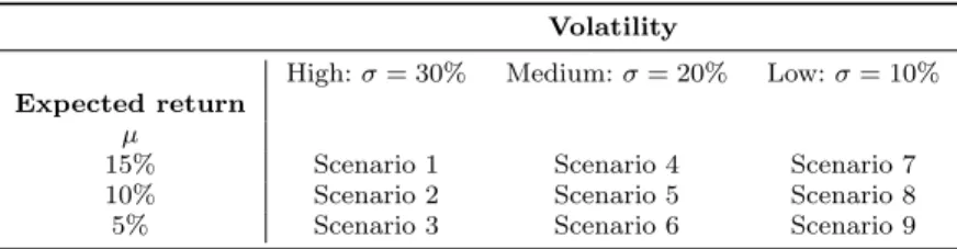
We use standard Monte Carlo methods to simulate the evolution of the risky asset for a variety of 9 different scenarios – see Table 2. The continuous compound stock market returns are generated 100,000 times for each scenario, using the Black and Scholes (1973) model, a one-year time horizon with daily rebalancing (252 trading days), a floor at 100%, and a risk-free rate of 5%.4
The risky asset dynamics are, thus, given by
dSt= µStdt+ σStWt ⇔ d(lnS) = (µ −
σ2
2 )dt + σdWt, (11) where µ and σ are constant and W is a Wiener process.
For each scenario we start by evaluating the performance of portfolio insurance strategies and bench-mark investments, and then evaluate each of them from the point of view of an investor with EUT, PT or CPT preferences.
The above 9 market scenarios – with high, medium and low volatility; high, medium and equivalent risk-free equity returns – allow us to capture a large span of possible bear and bull market conditions.
3 The smoothing of curves are weighting functions, assuming that the value function is linear.
Table 2 Stock market scenarios
Volatility
High: σ = 30% Medium: σ = 20% Low: σ = 10% Expected return
µ
15% Scenario 1 Scenario 4 Scenario 7
10% Scenario 2 Scenario 5 Scenario 8
5% Scenario 3 Scenario 6 Scenario 9
Following most empirical studies on PI, our simulations do not consider tax, bid and offer spreads, nor transaction costs on the stock market. Although tax and transaction costs may impact performance and affect final wealth, the purpose of this study is the comparison of the ability of the different frameworks – EUT, PT and CPT – to explain investor preferences across investment strategies but along the same simulated paths. See Leland (1985) for further discussion on the matter.
Contrary to the studies of Dichtl and Drobetz (2011), Do and Faff (2004), and Cesari and Cremonini (2003), we do not apply any filter on portfolio shifts (single or cumulative), in order to avoid biased comparisons. The time horizon of the investment period is one year, which is the standard maturity in retail and institutional markets.
3.3 Investment Strategies
The portfolio insurance strategies considered are:
1. Stop Loss Portfolio Insurance (SLPI) 2. Option Based Portfolio Insurance (OBPI)
3. Constant Proportion Portfolio Insurance with m = 1 (CPPI1) 4. Constant Proportion Portfolio Insurance with m = 3 (CPPI3) 5. Time Invariant Portfolio Protection (TIPP)
The benchmark non-PI strategies are: 6. Passive stock market strategy (Risky asset) 7. Portfolio with risky and riskless assets (50:50) 8. Risk-free cash market deposit (Riskless asset).
Given the evolution of the risky asset, the implementation of each strategy follows from the formulas in Section 2. In relation to CPPI 3 we opted for not allowing for short positions using a constraint on the risk-free asset: wrisk−f ree=
EBCP P I t
VCP P I t
∈ [0; 1], as in Benninga (1990), Do (2002), Annaert, Van Osselaer, and Verstraete (2009), and Dichtl and Drobetz (2011):
ESCP P It = max[min(m × Cut, VtCP P I), 0] . (12)
The constraint is included in each simulated path at the end of each trading day, when risky and risk-free asset allocations are recalculated. We also include this in the implementation of the TIPP – which can be seen as a variant of CPPI – so we can compare the strategies.
4 Results
Our results are of two different natures: performance and statistical results and investor decision results. This section finishes with a robustness analysis.
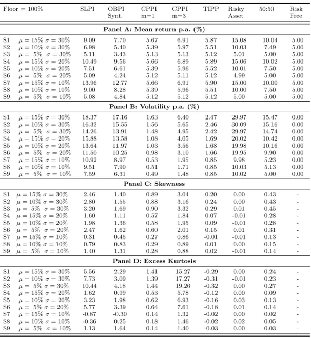
Table 3 Monte Carlo simulation results - Distributions of Returns.
This table shows descriptive statistics of the distributions of returns at maturity for the portfolio insurance and the benchmark strategies. Returns of the stock market were generated using a GBM. Portfolio insurance and benchmark strategies’ returns were simulated using Monte Carlo, and the risk-free rate was set at 5%. Stock returns were simulated daily for a period of one year with 252 trading days. The returns were simulated 100,000 times for each of the 9 scenarios presented in Table 2.
Floor = 100% SLPI OBPI
Synt. CPPI m=1 CPPI m=3 TIPP Risky Asset 50:50 Risk Free Panel A: Mean return p.a. (%)
S1 µ = 15% σ = 30% 9.09 7.70 5.67 6.91 5.87 15.08 10.04 5.00 S2 µ = 10% σ = 30% 6.98 5.40 5.39 5.97 5.51 10.03 7.49 5.00 S3 µ = 5% σ = 30% 5.11 3.43 5.13 5.13 5.12 5.01 5.00 5.00 S4 µ = 15% σ = 20% 10.49 9.56 5.66 6.89 5.89 15.06 10.02 5.00 S5 µ = 10% σ = 20% 7.51 6.61 5.39 5.96 5.52 10.01 7.50 5.00 S6 µ = 5% σ = 20% 5.09 4.24 5.12 5.11 5.12 4.99 5.00 5.00 S7 µ = 15% σ = 10% 13.96 12.77 5.66 6.91 5.90 15.00 10.00 5.00 S8 µ = 10% σ = 10% 9.00 8.28 5.39 5.96 5.51 10.00 7.50 5.00 S9 µ = 5% σ = 10% 5.08 4.84 5.12 5.12 5.12 5.00 5.00 5.00
Panel B: Volatility p.a. (%)
S1 µ = 15% σ = 30% 18.37 17.16 1.63 6.40 2.47 29.97 15.47 0.00 S2 µ = 10% σ = 30% 16.32 15.55 1.56 5.65 2.46 30.09 15.16 0.00 S3 µ = 5% σ = 30% 14.26 13.91 1.48 4.95 2.42 29.97 14.74 0.00 S4 µ = 15% σ = 20% 15.88 13.58 1.08 4.05 1.69 20.02 10.42 0.00 S5 µ = 10% σ = 20% 13.64 11.97 1.03 3.56 1.68 19.98 10.16 0.00 S6 µ = 5% σ = 20% 11.50 10.25 0.98 3.10 1.66 19.95 9.90 0.00 S7 µ = 15% σ = 10% 10.92 8.97 0.53 1.95 0.85 9.98 5.23 0.00 S8 µ = 10% σ = 10% 9.51 7.90 0.51 1.71 0.85 10.03 5.13 0.00 S9 µ = 5% σ = 10% 7.59 6.31 0.49 1.48 0.85 10.02 5.00 0.00 Panel C: Skewness S1 µ = 15% σ = 30% 2.46 1.40 0.89 3.04 0.20 0.00 0.43 -S2 µ = 10% σ = 30% 2.80 1.55 0.88 3.16 0.24 0.00 0.43 -S3 µ = 5% σ = 30% 3.20 1.69 0.90 3.32 0.29 0.01 0.45 -S4 µ = 15% σ = 20% 1.60 1.11 0.57 1.84 0.07 -0.01 0.28 -S5 µ = 10% σ = 20% 1.98 1.36 0.58 1.95 0.09 -0.01 0.28 -S6 µ = 5% σ = 20% 2.47 1.62 0.60 2.01 0.15 0.01 0.31 -S7 µ = 15% σ = 10% 0.31 0.45 0.27 0.86 -0.01 -0.01 0.13 -S8 µ = 10% σ = 10% 0.79 0.83 0.29 0.89 0.01 0.00 0.15 -S9 µ = 5% σ = 10% 1.40 1.31 0.28 0.88 0.02 -0.01 0.14
-Panel D: Excess Kurtosis
S1 µ = 15% σ = 30% 5.56 2.29 1.41 15.27 -0.29 0.00 0.24 -S2 µ = 10% σ = 30% 7.73 3.09 1.39 17.27 -0.31 -0.01 0.23 -S3 µ = 5% σ = 30% 10.44 4.18 1.44 19.26 -0.32 0.00 0.27 -S4 µ = 15% σ = 20% 1.62 0.99 0.53 5.78 -0.12 0.00 0.09 -S5 µ = 10% σ = 20% 3.23 1.98 0.62 6.93 -0.16 0.03 0.13 -S6 µ = 5% σ = 20% 5.77 3.39 0.64 7.61 -0.18 0.01 0.14 -S7 µ = 15% σ = 10% -0.87 -0.30 0.14 1.32 -0.02 0.00 0.02 -S8 µ = 10% σ = 10% -0.36 0.25 0.18 1.46 -0.02 0.02 0.05 -S9 µ = 5% σ = 10% 1.13 1.64 0.14 1.40 -0.03 0.00 0.03
-4.1 Performance and statistical results
Table 3 presents descriptive statistics on the distribution of returns of the various investment strategies for the different scenarios. Although the descriptive statistics are clearly not sufficient to conclude on the best portfolio insurance strategy, specially when the focus is on wealth protection or potential wealth increase (Annaert, Van Osselaer, and Verstraete (2009)), it is interesting to point results under several market conditions.
The annual expected return is presented in Panel A of Table 3 . In relation to expected returns in three bullish market conditions (scenarios 1-2, 4-5 and 7-8), holding the risky asset delivers the highest expected
return. Amongst the portfolio insurance strategies, the SLPI is the one with the highest expected return. The OBPPI is better than the unleveraged CPPI(m = 1), when market presents high returns, which is explained by the cost of protection that is accommodated in markets with high expected returns. The TIPP, with the ability to protect intermediary gains, presents the second lowest expected returns, amongst the portfolio insurance strategies, due to the cost of “cashing in” the intermediary upward movements of the risky asset. However, in depressed markets it tends to present better performance, excluding the unleveraged CPPI. The reason for the dominant results of the passive stock market strategy in bullish markets, compared with any of the portfolio insurance strategies, lies on the protection cost of downside risk, which is implicit on the latter. In a neutral market (Scenarios 3, 6 and 9), expected returns from the simulated strategies are all very similar, except for the OBPI, which penalizes returns due to volatility.
The annual volatilities are presented in Panel B of Table 3. The results are dependent on volatility parameter we set for the scenarios. TIPP and unleveraged CPPI are the portfolio insurance strategies with the lowest volatility in all scenarios. Regarding the benchmark strategies, naturally, the 50 : 50 strategy delivers the lowest volatility (except for the case of risk-free asset). The characteristic of moving up the floor of TIPP limits the dispersion of the returns at maturity, which gives the investor the lowest volatile strategy in all scenarios, except in the case of unleveraged CPPI. A particular feature of the SLPI strategy is that volatility decreases as scenarios change from more unstable market conditions to less volatile market (in relation to expected returns), due to the lower probability of activating stop loss orders.
The skewness measure is presented in Panel C of Table 3. Return distributions with positive skewness have frequent small losses, and some large gains; whereas, those with negative skewness have frequent small gains, and some large negative returns. Due to the characteristics of portfolio insurance strategies, we expect the results to show positive skewness, which was what was obtained. The SLPI return distri-butions have the highest skewness, as the loss cutting features make these distridistri-butions very right tailed. However, this does not occur in all scenarios, as the more bullish, and volatile, the market, the bigger the probability of the stop loss order being activated, and in these situations, the leveraged CPPI (m = 3) strategy has the most right tailed returns distribution.
The excess kurtosis results are presented in Panel D of Table 3. Higher kurtosis means that variance results from infrequent extreme deviations, rather than frequent modest deviations. As expected, return distribution of the benchmark strategies are mesokurtic, because the returns follow a lognormal distribu-tion. The TIPP return distributions are near mesokurtic in all scenarios, due to the fact that a dynamic floor limits deviations. In scenarios 7 to 9, in particular, the Stop Loss strategy is near mesokurtic, since low volatility and high returns make it less probable to execute the stop loss order, thus becoming a proxy of the lognormal return distribution. A leptokurtic distribution has more returns around the mean, but with large deviations. The return distributions of portfolio insurance strategies, in general, have leptokurtic behaviour and in the scenarios with the highest volatility we observe higher excess kurtosis.
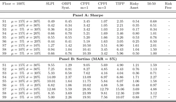
Table 4 presents the results for the performance ratios of Sharpe (1994) and Sortino and Van Der Meer (1991). The Sharpe ratio measures excess return per unit of risk (volatility). The higher the ratio, the better the performance adjusted by the risk. The ratio is given by
Sharpe Ratio =r¯p− rf σp
, (13)
where ¯rp is the expected return of the portfolio, σp is the volatility of portfolio and rf is the risk-free
interest rate of the market.
The Sortino ratio measures the risk-adjusted return of an investment (Sortino and Price, 1994), and is a modification of the Sharpe ratio, penalizing only those returns falling below an investor’s required rate of return, while the Sharpe ratio penalizes both upside and downside volatility equally. Though both ratios measure an investment’s risk-adjusted returns, they do so in significantly different ways, which will frequently lead to differing conclusions, regarding to the true nature of the investment’s return-generating efficiency. The Sortino ratio is commonly used to compare the risk adjusted performance of strategies with differing risk and return profiles. As most investors consider risk as the probability of not attaining the target return, this is an important measure for the downside risk. The Sortino ratio is given by
Sortino Ratio =r¯p− M AR σd
Table 4 Monte Carlo simulation results - Performance ratios
This table shows the results of performance (Sharpe and Sortino ratios) for the returns at maturity for the portfolio insurance and benchmark strategies. Returns of the stock market were generated using a GBM. Portfolio strategies returns and benchmark strategies were simulated using Monte Carlo, and the risk-free rate was set at 5%. Stock returns were simulated daily for a period of one year, with 252 trading days. The returns were simulated 100,000 times for each of the 9 scenarios presented in Table 2.
Floor = 100% SLPI OBPI
Synt. CPPI m=1 CPPI m=3 TIPP Risky Asset 50:50 Risk Free Panel A: Sharpe S1 µ = 15% σ = 30% 0.49 0.45 3.45 1.07 2.35 0.54 0.68 -S2 µ = 10% σ = 30% 0.42 0.34 3.42 1.05 2.21 0.35 0.51 -S3 µ = 5% σ = 30% 0.36 0.24 3.42 1.03 2.10 0.17 0.34 -S4 µ = 15% σ = 20% 0.66 0.70 5.21 1.69 3.46 0.80 1.01 -S5 µ = 10% σ = 20% 0.55 0.55 5.20 1.66 3.26 0.53 0.76 -S6 µ = 5% σ = 20% 0.44 0.41 5.18 1.63 3.05 0.25 0.50 -S7 µ = 15% σ = 10% 1.27 1.42 10.50 3.51 6.90 1.61 2.01 -S8 µ = 10% σ = 10% 0.94 1.04 10.41 3.45 6.43 1.04 1.50 -S9 µ = 5% σ = 10% 0.66 0.76 10.39 3.42 5.96 0.50 1.00
-Panel B: Sortino (MAR = 5%)
S1 µ = 15% σ = 30% 9.55 1.29 9.05 5.69 4.90 1.21 1.59 -S2 µ = 10% σ = 30% 7.25 0.91 8.27 4.85 4.43 0.76 1.13 -S3 µ = 5% σ = 30% 5.33 0.58 7.62 4.16 4.04 0.36 0.71 -S4 µ = 15% σ = 20% 14.09 2.37 13.09 6.97 6.86 1.71 2.27 -S5 µ = 10% σ = 20% 10.01 1.64 11.75 5.84 6.07 1.06 1.58 -S6 µ = 5% σ = 20% 6.82 1.06 10.62 4.88 5.38 0.48 0.97 -S7 µ = 15% σ = 10% 12.88 5.59 28.95 12.79 15.06 3.69 4.88 -S8 µ = 10% σ = 10% 8.35 3.69 23.99 9.81 12.36 2.09 3.12 -S9 µ = 5% σ = 10% 5.00 2.26 19.91 7.56 10.07 0.88 1.77
-where ¯rp is the expected return of the portfolio, M AR is the target return defined by the investor for the
portfolio (in some cases it is named the minimum acceptable return), and σd is the downside deviation
volatility of portfolio, that can be interpreted as the annualized standard deviation of returns below the target. The formula for the σd is
σd= v u u t n X i=1 min[(ri− M AR), 0]2 n . (15)
In all market scenarios the best Sharpe ration is given by the unleveraged CPPI (m = 1) strategy, which dominates all the other strategies. For the Sortino ration, In bullish and volatile markets, because the ratio penalizes the downside, the SLPI delivers the best risk-adjusted return. However, in the majority of market conditions, the unleveraged CPPI delivers the highest Sortino ratio, as the returns are right tailed.
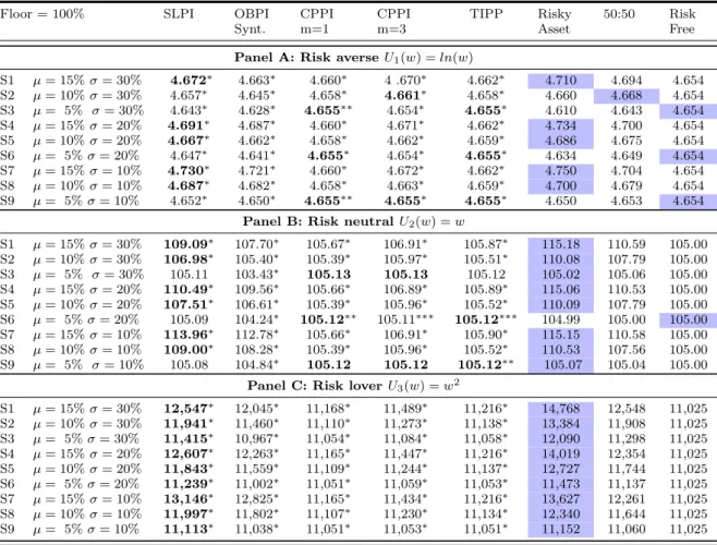
4.2 Investor decision results
The results for EUT investors are depicted in Table 5. The results for a risk averse investor are presented in Panel A of Table 5. In bullish markets (Scenarios 1, 4 and 7), for a risk averse investor, the highest utility is obtained from a passive stock market portfolio. The reason for this outcome is that the passive stock market delivers the highest expected wealth at maturity. Regarding portfolio insurance strategies, SLPI is the strategy that delivers the highest utility. When the market is neutral (Scenarios 3, 6 and 9), the results are inconclusive, as there is no dominant strategy between PI and benchmark strategies. The results for the risk neutral investor are presented in Panel B of Table 5. In market neutral conditions (Scenarios 3, 6 and 9), utility value is very similar amongst all strategies, except for the Synthetic OBPI, where the utility values are the lowest. In this strategy, due to the costs of protection, the lower the
volatility, the higher the utility value. Although very similar, the passive stock market strategy delivers the highest utility. When market conditions are very positive (Scenarios 1-2, 4-5 and 7-8) investors should choose the passive stock market investment in order to maximize utility. The results for a risk seeking investor are presented in Panel C of Table 5. The results are very interesting, because, as expected, investor should choose a passive stock market strategy for all market conditions. In any scenario, for a risk loving investor, portfolio insurance strategies should not be appealing options, as the upward movement is only partial. In this framework, investing in the equity market to collect a risk premium provides the best utility choice. Overall, our EUT results are in line with what would be expected from the previous literature. I.e, our results show no evidence that PI strategies are appealing to risk averse investors under this setup.
Table 5 Monte Carlo simulation results - EUT
This table shows the results of three utility functions (U1, U2, U3) representative of investors’ attitude towards
risk: aversion, neutrality and risk seeking. Utility functions are calculated using the portfolio value at maturity of the portfolio insurance and benchmark strategies. Wealth at maturity is the result of accumulated daily returns of each strategy. Returns of the stock market were generated using a GBM. Portfolio insurance and benchmark strategies’ returns were simulated using Monte Carlo, and the risk-free rate was set at 5%. Stock returns were simulated daily for a period of one year, with 252 trading days. The returns were simulated 100,000 times for each of the 9 scenarios presented in Table 2. The null hypothesis in the paired t-test is that the utility value of a portfolio insurance strategy is equal to that of the benchmark strategy with the highest utility value.
The test statistic is significant at a level ∗ = 1%, ∗∗ = 5% or, ∗ ∗ ∗ = 10%
Floor = 100% SLPI OBPI
Synt. CPPI m=1 CPPI m=3 TIPP Risky Asset 50:50 Risk Free Panel A: Risk averse U1(w) = ln(w)
S1 µ = 15% σ = 30% 4.672∗ 4.663∗ 4.660∗ 4 .670∗ 4.662∗ 4.710 4.694 4.654 S2 µ = 10% σ = 30% 4.657∗ 4.645∗ 4.658∗ 4.661∗ 4.658∗ 4.660 4.668 4.654 S3 µ = 5% σ = 30% 4.643∗ 4.628∗ 4.655∗∗ 4.654∗ 4.655∗ 4.610 4.643 4.654 S4 µ = 15% σ = 20% 4.691∗ 4.687∗ 4.660∗ 4.671∗ 4.662∗ 4.734 4.700 4.654 S5 µ = 10% σ = 20% 4.667∗ 4.662∗ 4.658∗ 4.662∗ 4.659∗ 4.686 4.675 4.654 S6 µ = 5% σ = 20% 4.647∗ 4.641∗ 4.655∗ 4.654∗ 4.655∗ 4.634 4.649 4.654 S7 µ = 15% σ = 10% 4.730∗ 4.721∗ 4.660∗ 4.672∗ 4.662∗ 4.750 4.704 4.654 S8 µ = 10% σ = 10% 4.687∗ 4.682∗ 4.658∗ 4.663∗ 4.659∗ 4.700 4.679 4.654 S9 µ = 5% σ = 10% 4.652∗ 4.650∗ 4.655∗∗ 4.655∗ 4.655∗ 4.650 4.653 4.654
Panel B: Risk neutral U2(w) = w
S1 µ = 15% σ = 30% 109.09∗ 107.70∗ 105.67∗ 106.91∗ 105.87∗ 115.18 110.59 105.00 S2 µ = 10% σ = 30% 106.98∗ 105.40∗ 105.39∗ 105.97∗ 105.51∗ 110.08 107.79 105.00 S3 µ = 5% σ = 30% 105.11 103.43∗ 105.13 105.13 105.12 105.02 105.06 105.00 S4 µ = 15% σ = 20% 110.49∗ 109.56∗ 105.66∗ 106.89∗ 105.89∗ 115.06 110.53 105.00 S5 µ = 10% σ = 20% 107.51∗ 106.61∗ 105.39∗ 105.96∗ 105.52∗ 110.09 107.79 105.00 S6 µ = 5% σ = 20% 105.09 104.24∗ 105.12∗∗ 105.11∗∗∗ 105.12∗∗∗ 104.99 105.00 105.00 S7 µ = 15% σ = 10% 113.96∗ 112.78∗ 105.66∗ 106.91∗ 105.90∗ 115.15 110.58 105.00 S8 µ = 10% σ = 10% 109.00∗ 108.28∗ 105.39∗ 105.96∗ 105.52∗ 110.53 107.56 105.00 S9 µ = 5% σ = 10% 105.08 104.84∗ 105.12 105.12 105.12∗∗ 105.07 105.04 105.00
Panel C: Risk lover U3(w) = w2
S1 µ = 15% σ = 30% 12,547∗ 12,045∗ 11,168∗ 11,489∗ 11,216∗ 14,768 12,548 11,025 S2 µ = 10% σ = 30% 11,941∗ 11,460∗ 11,110∗ 11,273∗ 11,138∗ 13,384 11,908 11,025 S3 µ = 5% σ = 30% 11,415∗ 10,967∗ 11,054∗ 11,084∗ 11,058∗ 12,090 11,298 11,025 S4 µ = 15% σ = 20% 12,607∗ 12,263∗ 11,165∗ 11,447∗ 11,216∗ 14,019 12,354 11,025 S5 µ = 10% σ = 20% 11,843∗ 11,559∗ 11,109∗ 11,244∗ 11,137∗ 12,727 11,744 11,025 S6 µ = 5% σ = 20% 11,239∗ 11,002∗ 11,051∗ 11,059∗ 11,053∗ 11,473 11,137 11,025 S7 µ = 15% σ = 10% 13,146∗ 12,825∗ 11,165∗ 11,434∗ 11,216∗ 13,627 12,261 11,025 S8 µ = 10% σ = 10% 11,997∗ 11,802∗ 11,107∗ 11,230∗ 11,134∗ 12,340 11,644 11,025 S9 µ = 5% σ = 10% 11,113∗ 11,038∗ 11,051∗ 11,053∗ 11,051∗ 11,152 11,060 11,025
Table 6 Monte Carlo simulation results - Prospect and Cumulative Prospect Theories
This table shows the results of (mean or cumulative) prospect value. Prospect values are calculated using the portfolio gains and losses, relative to a reference point (100 or 0% return) at maturity of the portfolio insurance and benchmark strategies. Gains and losses at maturity are the result of the accumulated daily returns of each strategy. Returns of the stock market were generated using a GBM. Portfolio insurance and benchmark strategies’ returns were simulated using Monte Carlo, and the risk-free rate was set at 5%. Stock returns were simulated daily for a period of one year, with 252 trading days. The returns were simulated 100,000 times for each of the 9 scenarios presented in Table 2. The null hypothesis in the paired t-test is that the (mean or cumulative) prospect value of a portfolio insurance strategy is equal to that of the benchmark strategy with the highest prospect value.
The test statistic is significant at a level ∗ = 1%, ∗∗ = 5% or, ∗ ∗ ∗ = 10%
Floor = 100% SLPI OBPI
Synt. CPPI m=1 CPPI m=3 TIPP Risky Asset 50:50 Risk Free Panel A: Mean prospect value (λ = 1.0)
S1 µ = 15% σ = 30% 6.93∗ 6.42∗ 7.75∗ 8.65∗ 7.92∗ 11.61 10.50 7.16 S2 µ = 10% σ = 30% 5.43∗ 4.58∗ 7.45∗∗∗ 7.73∗ 7.51 6.43 7.70 7.16 S3 µ = 5% σ = 30% 3.63∗ 2.47∗ 7.12∗ 6.73∗ 7.02∗ 0.73 4.62 7.16 S4 µ = 15% σ = 20% 9.68∗ 9.85∗ 7.79∗ 9.02∗ 8.03∗ 15.22 11.95 7.16 S5 µ = 10% σ = 20% 6.82∗ 6.59∗ 7.45∗ 7.92∗ 7.56∗ 9.14 8.65 7.16 S6 µ = 5% σ = 20% 4.67∗ 4.27∗ 7.15∗ 6.99∗ 7.11∗ 3.52 5.64 7.16 S7 µ = 15% σ = 10% 14.96∗ 14.36∗ 7.79∗ 9.15∗ 8.06∗ 17.53 12.84 7.16 S8 µ = 10% σ = 10% 9.98∗ 9.69∗ 7.47∗ 8.08∗ 7.60∗ 11.76 9.77 7.16 S9 µ = 5% σ = 10% 5.74∗ 5.92∗ 7.16∗ 7.12∗ 7.15∗ 5.68 6.58 7.16
Panel B: Mean prospect value (λ = 2.25)
S1 µ = 15%; σ = 30% 5.10∗ 1.11∗ 7.75∗ 8.65∗ 7.92∗ 0.74 6.45 7.16 S2 µ = 10% σ = 30% 3.52∗ -0.87∗ 7.45∗ 7.73∗ 7.51∗ -7.33 2.48 7.16 S3 µ = 5% σ = 30% 1.65∗ -3.28 7.12∗ 6.73∗ 7.02∗ -15.96 -1.77 7.16 S4 µ = 15% σ = 20% 8.60∗ 7.43∗ 7.79∗ 9.02∗ 8.03∗ 10.44 10.43 7.16 S5 µ = 10% σ = 20% 5.64∗ 3.65∗ 7.45∗ 7.92∗ 7.56∗ 1.96 6.27 7.16 S6 µ = 5% σ = 20% 3.38∗ 1.09∗ 7.15∗ 6.99∗ 7.11∗ -6.44 2.23 7.16 S7 µ = 15% σ = 10% 14.69∗ 14.08∗ 7.79∗ 9.15∗ 8.06∗ 16.91 12.75 7.16 S8 µ = 10% σ = 10% 9.61∗ 9.16∗ 7.47∗ 8.08∗ 7.60∗ 10.19 9.51 7.16 S9 µ = 5% σ = 10% 5.21∗ 5.15∗ 7.16∗ 7.12∗ 7.15∗ 2.07 5.81 7.16
Panel C: Mean cumulative prospect value (λ = 2.25)
S1 µ = 15% σ = 30% 17.04∗ 7.00∗ 7.86∗ 11.61∗ 7.20∗∗ 6.96 7.65 7.16 S2 µ = 10% σ = 30% 14.34∗ 3.65∗ 7.52∗ 10.25∗ 6.88∗ -0.37 3.82 7.16 S3 µ = 5% σ = 30% 11.30∗ 0.14∗ 5.21∗ 8.70∗ 6.68∗ -8.06 -0.18 7.16 S4 µ = 15% σ = 20% 15.65∗ 9.08∗ 4.13∗ 9.13∗ 7.71∗ 10.48 9.44 7.16 S5 µ = 10% σ = 20% 12.53∗ 5.31∗ 7.49∗ 8.84∗ 7.26∗ 3.42 5.82 7.16 S6 µ = 5% σ = 20% 9.65∗ 1.37∗ 3.70∗ 7.06∗∗ 6.80∗ -4.12 1.97 7.16 S7 µ = 15% σ = 10% 15.50∗∗ 12.98∗ 2.52∗ 6.58∗ 8.01∗ 15.83 11.98 7.16 S8 µ = 10% σ = 10% 11.25∗ 8.36∗ 7.55∗ 8.21∗ 7.53∗ 8.67 8.42 7.16 S9 µ = 5% σ = 10% 7.56∗ 3.60∗ 7.22∗ 7.19∗∗ 4.63∗ 1.04 4.70 7.16
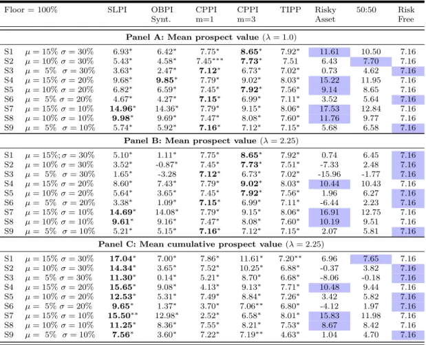
The results for the prospect theories – PT and CPT – are presented in Table 6. In Panel A of Table 6 we use mean prospect with λ = 1, which means that reaction to losses is not different from the reaction to gains. In Panel B, we incorporate a different loss reaction, using λ = 2.25. In both situations, there is no distinct weighting of the gains, and losses; therefore, we calculate the simple mean of the simulated prospect values. In Panel C of Table 6, we incorporate the cumulative probability weightings.
The results of Panel A of Table 6 present the prospect values for an investor with similar reactions to gains and losses. The prospect values show that, for bullish market conditions (scenarios 1-2, 4-5, and 7-8), a passive stock market strategy yields the best global results. In neutral conditions (scenarios 3, 6 and 9), the unleveraged CPPI strategy is the best choice. The leveraged CPPI and TPPI, as well as the risk-free investment have prospect values very similar to unleveraged CPPI. In Panel B of Table 6, we incorporate the loss reaction for investors in valuing outcomes, and find that results become more favourable to portfolio insurance strategies. In some bullish market conditions with medium to low volatility, a passive stock market investment delivers high prospect value, as high negative returns are not frequent. In market conditions with high and medium expected returns and volatility, portfolio insurance strategies yields high
prospect values for investors. In most cases, leveraged CPPI is the best strategy. When market conditions are relatively stable, and with high expected returns (scenarios 7 and 8), a risky investment continues to deliver the highest prospect value. Except for the bearish market conditions, where risk-free investment has the highest value, and the low to medium volatile markets with high expected returns, where a passive stock market strategy yields the best result, in all other scenarios portfolio insurance strategies are the best choices. The results of Panel C in Table 6 present the cumulative prospect values. There is only one scenario where benchmark strategies dominate portfolio insurance strategies: scenario 7, where the best choice is a passive stock market strategy. The SLPI strategy dominates all other strategies in the remaining scenarios. The results support a possible explanation for the popularity of portfolio insurance on a behavioural finance context, and especially regarding the preference of na¨ıve strategies as the SLPI. Amongst PI strategies, the SLPI is always the best choice. The way investors react against prospects with losses or gains, and also on the different valuation of low or high probabilities, is not captured in an expected utility theory. Hence, this is not a complete framework to explain the attractiveness of portfolio insurance. On the contrary, a prospect theory approach may support the longevity of strategies that offer protection on the downside and, at the same time, keep a potential to benefit from the upside.
4.3 Robustness Tests
We perform several tests in order to assess the adherence of the results. We begin by changing the floor from 100% to 80% and re-run the model. On a second analysis, we test the parameters of CPT used by Tversky and Kahneman (1992): we change these assumptions in order to increase the overweight of small probability events in negative outcomes (we change the δ from 0.69 to 0.77, and the γ from 0.61 to 0.44, while keeping the α constant at 0.88), in line with parameters defined in the experiment by Gonzalez and Wu (1999) regarding the weighting process. The final tests are related with the changes of risk-free rates (we stress the risk-free rate by 150 basis points, from 5% to 3.5% and from 5% to 6.5%) in order to check the impact on investor choices.
Floor at 80%
We elaborate a complete rerun of the model using a floor of 80% on the portfolio insurance strategies. The results confirm the overall findings when floor is at 100%.
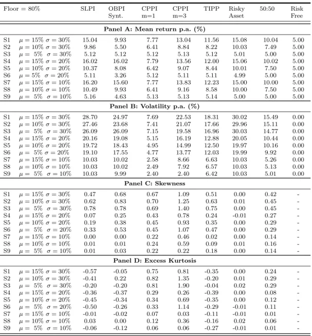
Table 7 presents the performance indicator. As expected, the portfolio insurance strategies yield wider range of returns and high volatility. The new conditions result in positive skewness for portfolio insurance strategies, but bigger exposure to risky assets leads to a less positive skew distribution.
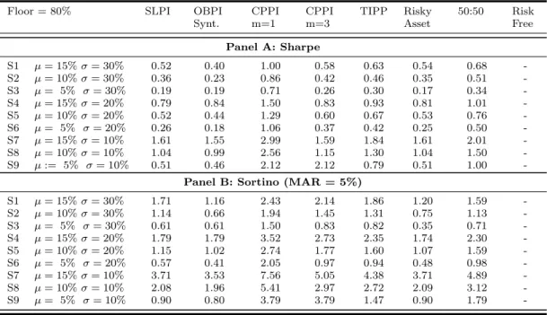
The Sharpe ratio results are presented in Table 8. The unleveraged CPPI with a lower floor continues to yield the best reward to risk, overall. However, a greater exposure to risk, with increasing probability of losses, results on a lower Sharpe ratio for portfolio insurance strategies. The results of the Sortino ratio show high dispersion, as the chances of negative outcomes are bigger. Comparing these results with the Sortino ratio for portfolio insurance strategies with a floor of 100%, we observe lower values, as expected.
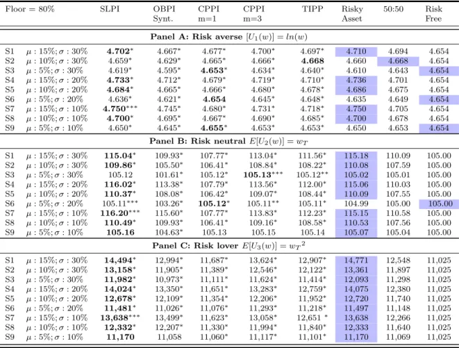
The results under the expected utility framework are presented in Table 9.
For a risk averse investor, indicated in Panel A of Table 9, when the floor is changed from 100% to 80%, the results confirm, overall, the utility derived from the passive stock market strategy, and, also, the risk-free investment. However, with the new floor, in market conditions with low volatility, SLPI strategy and unleveraged CPPI yield a higher utility value than benchmark strategies.
The results for a risk neutral investor, presented in Panel B of Table 9, points that portfolio insurance strategies do not yield higher utility to a neutral investor. In the case of an 80% floor, a SLPI becomes a possible choice for a risk neutral investor, in high expected market returns with low volatility, as utility is very similar to a passive stock market strategy –as expected, because the probability of executing the stop loss order is lower. For a risk loving investor, the reduction of the floor does not change the results. They are very similar to results from Panel B of Table 5, and the passive stock market strategy yields the highest utility for all bullish or neutral scenarios.
Overall results by portfolio insurance strategies, when the floor is reduced, and, consequently, an increasing exposure to risky assets is allowed, present higher utility values. However, this increase is not enough to change investors choices. The explanation for the popularity of portfolio insurance strategies
Table 7 Monte Carlo simulation results - Distributions of Returns
This table shows descriptive statistics of the distributions of returns at maturity for the portfolio insurance and the benchmark strategies. Returns of the stock market were generated using a GBM. Portfolio insurance and benchmark strategies’ returns were simulated using Monte Carlo, and the risk-free rate was set at 5%. Stock returns were simulated daily for a period of one year with 252 trading days. The returns were simulated 100,000 times for each of the 9 scenarios presented in Table 2.
Floor = 80% SLPI OBPI
Synt. CPPI m=1 CPPI m=3 TIPP Risky Asset 50:50 Risk Free Panel A: Mean return p.a. (%)
S1 µ = 15% σ = 30% 15.04 9.93 7.77 13.04 11.56 15.08 10.04 5.00 S2 µ = 10% σ = 30% 9.86 5.50 6.41 8.84 8.22 10.03 7.49 5.00 S3 µ = 5% σ = 30% 5.12 5.12 5.12 5.13 5.12 5.01 5.00 5.00 S4 µ = 15% σ = 20% 16.02 16.02 7.79 13.56 12.00 15.06 10.02 5.00 S5 µ = 10% σ = 20% 10.37 8.08 6.42 9.07 8.44 10.01 7.50 5.00 S6 µ = 5% σ = 20% 5.11 3.26 5.12 5.11 5.11 4.99 5.00 5.00 S7 µ = 15% σ = 10% 16.20 15.60 7.77 13.83 12.23 15.00 10.00 5.00 S8 µ = 10% σ = 10% 10.49 9.93 6.41 9.16 8.58 10.00 7.50 5.00 S9 µ = 5% σ = 10% 5.16 4.63 5.13 5.13 5.14 5.00 5.00 5.00
Panel B: Volatility p.a. (%)
S1 µ = 15% σ = 30% 28.70 24.97 7.69 22.53 18.31 30.02 15.49 0.00 S2 µ = 10% σ = 30% 27.46 23.68 7.41 21.07 17.66 29.96 15.11 0.00 S3 µ = 5% σ = 30% 26.09 26.09 7.15 19.58 16.96 30.03 14.77 0.00 S4 µ = 15% σ = 20% 20.16 19.08 5.15 16.19 12.88 20.05 10.44 0.00 S5 µ = 10% σ = 20% 19.72 18.43 4.95 14.99 12.50 19.97 10.16 0.00 S6 µ = 5% σ = 20% 19.10 17.55 4.77 13.77 12.03 19.99 9.92 0.00 S7 µ = 15% σ = 10% 10.03 10.02 2.58 8.66 6.63 10.03 5.26 0.00 S8 µ = 10% σ = 10% 10.03 10.02 2.49 7.92 6.57 10.03 5.13 0.00 S9 µ = 5% σ = 10% 10.03 9.99 2.40 2.40 6.42 10.03 5.01 0.00 Panel C: Skewness S1 µ = 15% σ = 30% 0.47 0.68 0.67 1.09 0.51 0.00 0.42 -S2 µ = 10% σ = 30% 0.62 0.83 0.70 1.25 0.63 0.01 0.45 -S3 µ = 5% σ = 30% 0.78 0.78 0.69 1.40 0.75 0.00 0.45 -S4 µ = 15% σ = 20% 0.07 0.25 0.43 0.78 0.24 -0.01 0.27 -S5 µ = 10% σ = 20% 0.19 0.38 0.45 0.93 0.35 0.00 0.29 -S6 µ = 5% σ = 20% 0.33 0.53 0.45 1.07 0.47 0.00 0.29 -S7 µ = 15% σ = 10% 0.00 0.00 0.22 0.46 0.02 0.00 0.14 -S8 µ = 10% σ = 10% 0.01 0.01 0.24 0.59 0.09 0.01 0.16 -S9 µ = 5% σ = 10% 0.01 0.03 0.22 0.22 0.18 0.00 0.14
-Panel D: Excess Kurtosis
S1 µ = 15% σ = 30% -0.57 -0.05 0.75 0.81 -0.35 0.00 0.24 -S2 µ = 10% σ = 30% -0.41 0.22 0.82 1.35 -0.20 0.01 0.29 -S3 µ = 5% σ = 30% -0.20 -0.20 0.81 1.90 -0.04 0.02 0.29 -S4 µ = 15% σ = 20% -0.36 -0.37 0.29 0.26 -0.39 0.00 0.08 -S5 µ = 10% σ = 20% -0.45 -0.34 0.34 0.69 -0.35 0.00 0.12 -S6 µ = 5% σ = 20% -0.50 -0.26 0.33 1.14 -0.29 -0.01 0.11 -S7 µ = 15% σ = 10% -0.01 -0.02 0.07 0.03 -0.11 -0.01 0.01 -S8 µ = 10% σ = 10% 0.03 0.00 0.12 0.36 -0.16 0.02 0.06 -S9 µ = 5% σ = 10% -0.06 -0.12 0.06 0.06 -0.27 -0.01 0.01
-is, according with our simulation, not explained under the framework of expected utility theory, even if we increase the upside potential.
Table 8 Monte Carlo simulation results - Performance ratios
This table shows the results of performance ratios (Sharpe and Sortino) for the returns at maturity for the portfolio insurance and benchmark strategies. Returns of the stock market were generated using a GBM. Portfolio insurance and benchmark strategies’ returns were simulated using Monte Carlo and the risk-free rate was set at 5%. Stock returns were simulated daily for a period of one year, with 252 trading days. The returns were simulated 100,000 times for each of the 9 scenarios presented in Table 2.
Floor = 80% SLPI OBPI
Synt. CPPI m=1 CPPI m=3 TIPP Risky Asset 50:50 Risk Free Panel A: Sharpe S1 µ = 15% σ = 30% 0.52 0.40 1.00 0.58 0.63 0.54 0.68 -S2 µ = 10% σ = 30% 0.36 0.23 0.86 0.42 0.46 0.35 0.51 -S3 µ = 5% σ = 30% 0.19 0.19 0.71 0.26 0.30 0.17 0.34 -S4 µ = 15% σ = 20% 0.79 0.84 1.50 0.83 0.93 0.81 1.01 -S5 µ = 10% σ = 20% 0.52 0.44 1.29 0.60 0.67 0.53 0.76 -S6 µ = 5% σ = 20% 0.26 0.18 1.06 0.37 0.42 0.25 0.50 -S7 µ = 15% σ = 10% 1.61 1.55 2.99 1.59 1.84 1.61 2.01 -S8 µ = 10% σ = 10% 1.04 0.99 2.56 1.15 1.30 1.04 1.50 -S9 µ := 5% σ = 10% 0.51 0.46 2.12 2.12 0.79 0.51 1.00
-Panel B: Sortino (MAR = 5%)
S1 µ = 15% σ = 30% 1.71 1.16 2.43 2.14 1.86 1.20 1.59 -S2 µ = 10% σ = 30% 1.14 0.66 1.94 1.45 1.31 0.75 1.13 -S3 µ = 5% σ = 30% 0.61 0.61 1.50 0.83 0.82 0.35 0.71 -S4 µ = 15% σ = 20% 1.79 1.79 3.52 2.73 2.35 1.74 2.30 -S5 µ = 10% σ = 20% 1.15 1.02 2.74 1.77 1.60 1.07 1.59 -S6 µ = 5% σ = 20% 0.57 0.41 2.05 0.97 0.94 0.48 0.98 -S7 µ = 15% σ = 10% 3.71 3.53 7.56 5.05 4.38 3.71 4.89 -S8 µ = 10% σ = 10% 2.08 1.96 5.41 2.97 2.72 2.09 3.12 -S9 µ = 5% σ = 10% 0.90 0.80 3.79 3.79 1.47 0.90 1.79
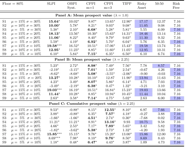
-The results of prospect values are presented in Table 10. -The outcomes of the simulation for portfolio insurance strategies with a floor set at 80% confirms the possibility of explaining the choices by investors for these type of strategies under the cumulative prospect valuation. The comparison is between investors with λ = 2.25, which represent different reactions to gains and losses.
The mean prospect values of Panel B in Tables 6 and 10 denote a consistent option of the investor for strategies with less chances of negative outcomes. There is evidence that, when a bigger exposure to risky assets in low volatile markets (scenarios 7 and 8) is allowed, the choice between a passive stock market and a SLPI strategy is almost indifferent. Since the return distributions of these two strategies tend to coincide, and present more chances of losses, the risk-free investments becomes more attractive. We also observe a shift from leveraged to unleveraged CPPI strategies for high and medium volatile markets (scenarios 1, 2, 4 and 5). In general, amongst portfolio insurance strategies, the more protective the strategies are, the more valuable to prospect investors.
The results for cumulative investors point to a possible explanation for some flight to safety when markets are neutral (scenarios 3, 6 and 9). In these market conditions, we can expect a change from SLPI to risk-free investments. In positive market expectations, independently of volatility, the cumulative value of leveraged CPPI strategies is higher than SLPI (scenarios 1-2, 4-5, and 8). The portfolio insurance strategies, under these market conditions, are still providing better results than benchmarking strategies. Results from Panel C of Tables 6 and 10, for positive market conditions (i.e. expected positive risk premium), strengthens the possibility that cumulative prospect theory explains investors’ choices. The specific decisions of portfolio insurance are, nonetheless, dependent on the market conditions and char-acteristics of each portfolio insurance strategy—e.g. the reduction of the percentage floor from 100% to 80% depicts a shift from SLPI to CPPI strategies.
Table 9 Monte Carlo simulation results - EUT
This table shows the results of three utility functions (U1; U2; U3) representative of investors’ attitude towards
risk: aversion, neutrality and risk seeking, respectively. Utility functions are calculated using the portfolio value at maturity of the portfolio insurance and benchmark strategies. Wealth at maturity is the result of accumulated daily returns of each strategy. Returns of the stock market were generated using a GBM. Portfolio insurance and benchmark strategies’ returns were simulated using Monte Carlo, and the risk-free rate was set at 5%. Stock returns were simulated daily for a period of one year, with 252 trading days. The returns were simulated 100,000 times for each of the 9 scenarios presented in Table 2. The null hypothesis in the paired t-test is that the utility value of a portfolio insurance strategy is equal to that of the benchmark strategy with the highest utility value.
The test statistic is significant at a level ∗ = 1%, ∗∗ = 5% or, ∗ ∗ ∗ = 10%
Floor = 80% SLPI OBPI
Synt. CPPI m=1 CPPI m=3 TIPP Risky Asset 50:50 Risk Free Panel A: Risk averse [U1(w)] = ln(w)
S1 µ : 15%; σ : 30% 4.702∗ 4.667∗ 4.677∗ 4.700∗ 4.697∗ 4.710 4.694 4.654 S2 µ : 10%; σ : 30% 4.659∗ 4.629∗ 4.665∗ 4.666∗ 4.668 4.660 4.668 4.654 S3 µ : 5%; σ : 30% 4.619∗ 4.595∗ 4.653∗ 4.634∗ 4.640∗ 4.610 4.643 4.654 S4 µ : 15%; σ : 20% 4.733∗ 4.712∗ 4.679∗ 4.719∗ 4.710∗ 4.736 4.701 4.654 S5 µ : 10%; σ : 20% 4.684∗ 4.665∗ 4.666∗ 4.680∗ 4.678∗ 4.686 4.675 4.654 S6 µ : 5%; σ : 20% 4.636∗ 4.621∗ 4.654 4.645∗ 4.648∗ 4.635 4.649 4.654 S7 µ : 15%; σ : 10% 4.750∗∗∗ 4.745∗ 4.680∗ 4.731∗ 4.718∗ 4.750 4.705 4.654 S8 µ : 10%; σ : 10% 4.700∗ 4.695∗ 4.667∗ 4.690∗ 4.685∗ 4.700 4.678 4.654 S9 µ : 5%; σ : 10% 4.650∗ 4.645∗ 4.655∗ 4.653∗ 4.653∗ 4.650 4.653 4.654
Panel B: Risk neutral E[U2(w)] = wT
S1 µ : 15%; σ : 30% 115.04∗ 109.93∗ 107.77∗ 113.04∗ 111.56∗ 115.18 110.09 105.00 S2 µ : 10%; σ : 30% 109.86∗ 105.50∗ 106.41∗ 108.84∗ 108.22∗ 110.08 107.59 105.00 S3 µ : 5%; σ : 30% 105.12 101.61∗ 105.12∗ 105.13∗∗∗ 105.12∗∗ 105.02 105.01 105.00 S4 µ : 15%; σ : 20% 116.02∗ 113.38∗ 107.79∗ 113.56∗ 112.00∗ 115.06 110.03 105.00 S5 µ : 10%; σ : 20% 110.37∗ 108.08∗ 106.42∗ 109.07∗ 108.44∗ 110.09 107.55 105.00 S6 µ : 5%; σ : 20% 105.11∗∗∗ 103.26∗ 105.12∗ 105.11∗∗ 105.11∗ 104.99 105.00 105.00 S7 µ : 15%; σ : 10% 116.20∗∗∗ 115.60∗ 107.77∗ 113.83∗ 112.23∗ 115.15 110.58 105.00 S8 µ : 10%; σ : 10% 110.49∗ 109.93∗ 106.41∗ 109.16∗ 108.58∗ 110.53 107.56 105.00 S9 µ : 5%; σ : 10% 105.16 104.63∗ 105.13 105.15 105.14 105.07 105.04 105.00
Panel C: Risk lover E[U3(w)] = wT2
S1 µ : 15%; σ : 30% 14,494∗ 12,994∗ 11,687∗ 13,624∗ 12,907∗ 14,771 12,548 11,025 S2 µ : 10%; σ : 30% 13,158∗ 11,905∗ 11,389∗ 12,546∗ 12,122∗ 13,361 11,897 11,025 S3 µ : 5%; σ : 30% 11,982∗ 10,973∗ 11,111∗ 11,624∗ 11,414∗ 12,093 11,298 11,025 S4 µ : 15%; σ : 20% 14,024∗ 13,350∗ 11,651∗ 13,283∗ 12,759∗ 14,075 12,380 11,025 S5 µ : 10%; σ : 20% 12,678∗ 12,109∗ 11,354∗ 12,206∗ 11,952∗ 12,720 11,740 11,025 S6 µ : 5%; σ : 20% 11,481∗ 11,026∗ 11,076∗ 11,293∗ 11,218∗ 11,497 11,148 11,025 S7 µ : 15%; σ : 10% 13,638∗∗∗ 13,499∗ 11,623∗ 13,058∗ 12,651∗ 13,638 12,266 11,025 S8 µ : 10%; σ : 10% 12,332∗ 12,207∗ 11,330∗ 11,994∗ 11,840∗ 12,333 11,640 11,025 S9 µ : 5%; σ : 10% 11,170 11,058 11,060∗ 11,117∗ 11,101∗ 11,170 11,069 11,025 Changing CPT parameters
The Table 11 presents the cumulative prospect value with changes on the parameters for the curvature and the elevation of the smoothing of curves. In this sensitivity analysis we modify the assumptions in order to increase the overweight of small probability events in negative outcomes (we change the δ from 0.69 to 0.77, and the γ from 0.61 to 0.44, while keeping the α constant at 0.88), in line with parameters defined in the experiment by Gonzalez and Wu (1999) regarding the weighting process.
The results on cumulative prospect values indicate portfolio insurance dominates benchmark strategies in all market conditions. The portfolio insurance strategy with higher value is the SLPI, since there is an overreaction to losses. Comparing the results with scenarios of Panel C in Table 6, we find that cumulative values are higher, and the downside risk aversion is managed using the same strategy – SLPI, hence confirming our results that prospect theory is a viable framework to explain portfolio insurance popularity.