J. Aerosp. Technol. Manag. vol.3 número1

Davidson Martins Moreira* Universidade Federal do Pampa

Bagé – Brazil [email protected]

Leonardo Barboza Trindade Universidade Federal do Rio Grande do Sul Porto Alegre – Brazil [email protected]

Gilberto Fisch Institute of Aeronautics and Space

São José dos Campos – Brazil [email protected]

Marcelo Romero de Moraes Universidade Federal do Pampa

Bagé – Brazil [email protected]

Rodrigo Martins Dorado Universidade Federal do Pampa

Bagé – Brazil [email protected]

Roberto Lage Guedes Institute of Aeronautics and Space

São José dos Campos – Brazil [email protected]

*author for correspondence

A multilayer model to simulate

rocket exhaust clouds

Abstract: This paper presents the MSDEF (Modelo Simulador da Dispersão de Eluentes de Foguetes, in Portuguese) model, which represents the solution for time-dependent advection-diffusion equation applying the Laplace transform considering the Atmospheric Boundary Layer as a multilayer system. This solution allows a time evolution description of the concentration ield emitted from a source during a release lasting time tr , and it takes into account deposition velocity, irst-order chemical reaction, gravitational settling, precipitation scavenging, and plume rise effect. This solution is suitable for describing critical events relative to accidental release of toxic, lammable, or explosive substances. A qualitative evaluation of the model to simulate rocket exhaust clouds is showed.

Keywords: Alcântara Launch Center, Advection-diffusion equation, Atmospheric dispersion.

INTRODUCTION

A model is an abstract idealization of a process involving one or more functions designed to simplify our description of the process. Constraints on the model include the availability and scope of the dataset; the mathematical approximation and limits of solution; and the complexity of analysis and data reduction that can be tolerated. In these considerations, we are interested in a diffusion model to provide a viable description

of the transport of rocket exhaust efluents in the atmosphere. The transport of the rocket exhaust efluents is characterized

by turbulent diffusion, in the atmosphere, which has not been uniquely formulated in the sense that a single basic physical

model capable of explaining all the signiicant aspects of the

transport process has not yet been proposed. The two general models are: the gradient transport model and the statistical one. Since atmospheric transport processes tend to be generally a nonstationary random process over periods of interest, and because normal meteorological data are incompatible with the statistical model, this approach is rejected in favor of the gradient transport model in the selection of an operational diffusion one. While the numerical and statistical techniques offer some vantages, especially in research investigations, the state of art of these transport techniques has not evolved

to the point where they offer a viable solution to operational

transport predictions rocket exhaust efluents for air quality

and environmental assessments; thus, our selection offers an analytical technique for diffusion predictions (Stephens and Stewart, 1977).

The burning of rocket engines during the irst few seconds

prior to and immediately following vehicle launches results in the formation of a large cloud of hot, buoyant exhaust products near the ground level, which subsequently rises and entrains ambient air until the temperature and density of the cloud reach an approximate equilibrium with ambient conditions. By convention, this cloud is referred to as the ground-cloud. The rocket engines also leave an exhaust trial from normal launches that extend throughout and beyond the troposphere depth. The National Aeronautics and Space Administration (NASA) has computational codes that are designed to calculate peak concentration, dosage and deposition (resulting from both gravitational settling and precipitation scavenging) downwind from normal and aborted launchings to use in mission planning activities and environmental assessments, pre-launch forecasts of the environmental effects of launch operations and post-launch environmental analysis (Bjorklund et al., 1982). Many of these models are based on the same steady-state Gaussian dispersion model concepts used by other ones. For sake of illustration, we cite the MSFC (Dumbauld et al., 1973),

Received on: 11/02/11 Accepted on: 10/03/11

REEDM (Bjorklund et al., 1982), RTVSM (Bjorklund, 1990), and OBODM (Bjorklund et al., 1998).

Recently, we take a step forward regarding the Gaussian concepts to simulate pollutant dispersion in atmosphere. The solution was obtained for a vertically inhomogeneous atmospheric boundary layer (ABL) of the time-dependent advection-diffusion equation, applying the Laplace transform, considering the ABL as a multilayer system. This technique is called advection-diffusion multilayer method (ADMM) and it is well established in the literature (Moreira et al., 2005a, b, c, d; Moreira et al., 2006).

Therefore, the aim of this paper is to report the construction of a new model based on ADMM model, now called MSDEF, to simulate rocket exhaust clouds.

For a better understanding, in the sequel, we briely

discuss the idea behind this method. The main feature of the ADMM approach consists on the following steps: stepwise approximation of the eddy diffusivity and wind speed; the Laplace transform application to the advection-diffusion equation in the x and t variables; semi-analytical solution of the linear ordinary equation set resulting in the Laplace transform application and construction of the pollutant concentration by the Laplace transform inversion, using the Gaussian quadrature

scheme. It is important to mention that, for the irst time,

the ADMM model (now MSDEF) is depending on time

release, deposition velocity, irst-order chemical reaction,

gravitational settling, and precipitation scavenging. This solution allows a time evolution description of

the concentration ield emitted from a source during a

release lasting time t_r. The model takes into account the plume rise formulation of the literature (Briggs, 1975) for convective conditions, which is included in the computational codes of the NASA. The code used by

NASA is the well-know rocket exhaust efluent diffusion

model (REEDM). The REEDM has been used to assess the environmental impact of Space Shuttle operation and

to support the irst launches of the Space Shuttle. The

dispersion models used in the REEDM code are based on Gaussian model concepts. The exhaust material, which is a mixture amongst CO, CO₂, HCl and alumina, that is, the most solid propellants exhausted gases, is assumed to be uniformly distributed in the vertical and to have a bivariate Gaussian distribution in the plane of the horizon at the point of cloud stabilization. The REEDM system is operationally used at Cape Canaveral to model the behavior of rocket exhaust clouds, and to evaluate the potential threat to health from the toxic gases present in those clouds.

PHYSICAL APPROACH

A tool for analysis of toxic dispersion in the USA and to support the release and evaluation of public risk is the 7.13 version of the REEDM (Bjorklund et al., 1982; Bjorklund, 1990; Bjorklund et al., 1998). Thus, this program was used as reference for modeling physics and mathematics of the problem in the development of MSDEF program. For more details about these approaches, see Bjorklund et al. (1982).

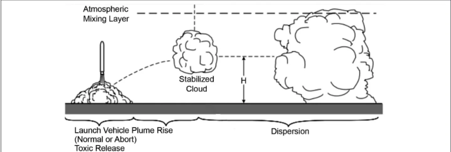
The main assumption used in the REEDM on the nature and behavior of the cloud released by the rocket is that it

can be initially deined as a single cloud that grows and

moves, but remains the same during the formation of its ascending phase. This concept is illustrated in Fig. 1, where it can be noticed that the model is designed for REEDM concentrations from the vertical position of the stabilized cloud.

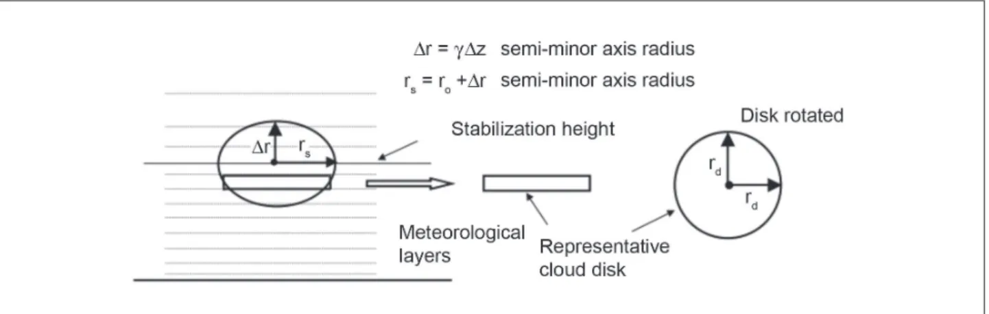
The aspect “multilayer” is still used in the REEDM and relates to the partitioning of cloud stabilized in “disks” of material from the cloud, represented by different meteorological levels at different altitudes. Typical levels are 20 to 50 m deep.

Since the cloud is deined and has reached the condition

of thermal stability with the atmosphere, it is partitioned into “disks”.The position of each disk with respect to the origin (launch pad) is determined based on the cloud’s

rise time through a sequence of layers, which are deined

using meteorological measuring levels obtained from a radiosonde. Each layer can have a single meteorological speed and wind direction that moves the disk into the same cloud. The concept of stabilized cloud partition is illustrated in Fig. 2.

The hypothesis of transport in a straight line used in the REEDM during the transport of clouds and phase

dispersion ignores the possibility of wind ields, which

can arise in complex mountainous terrain or may evolve during the passage of a sea breeze front or greater scale. Thus, it is recommended that the assumption of uniform wind is limited to the transport of the plume at distances that do not exceed 25 km. Therefore, the model does forecast REEDM concentration ranging from 5 to 10 km from the launch pad, so that this hypothesis is not a problem.

The REEDM assumes that all chemical reactions are completed before the combustion process of the cloud’s rise. A mass fraction is assigned to each constituent and the total mass of the source (cloud) is multiplied by this fraction to determine the total mass of each chemical component in the cloud. The molecular weight of each species is used to convert the mass concentration per unit volume (mg/m3_{) to part per million (ppm).}

The REEDM makes predictions of instantaneous and average concentration in time (typically a 10-minute average). In many situations, an average of one hour is made to compute the average concentrations. A shorter average time is appropriate to expose the cloud of the rocket, because the source (cloud) typically goes on a receiver with a time scale of ten minutes before the hour.

THE MATHEMATICAL MODEL

A typical problem with the advection-diffusion equation involves the solutions of problems corresponding to instantaneous and continuous sources of pollution. More precisely, considering a Cartesian coordinate system in which the x direction coincides with the one of the average wind, the time dependent advection-diffusion equation can be written as (Huang, 1979):

y

y "

© «ª ¹ »º © «ª ¹ C t u C x v C

z x K

C

x y K

C y

g x y

y y y y y y y y y y y y »»º © «ª ¹ »º y y y y z K C z S z (1)

Where C denotes the average concentration, K_x, K_y, K_z

are Cartesian components of eddy diffusivity, u is the longitudinal wind speed, v_g is the gravitational settling, and S is a source/sink term.

The analytical solution of the Eq. 1 can be obtained assuming (Huang, 1979):

C x y z t f x y t Cy x z t

( , , , )" ( , , ) ( , , ) (2)

The function f (x,y,t) can be expressed as:

f x y t y y

y

o

y

( , , )" exp©( )

« ª ¹ » º 1 2 2 2 2

UX X . (3)

Cy( , , )x z t is the solution of the following equation:

y

y "

© «ª ¹ »º C t u C x v C

z x K

C

x z K

C z y y g x y z y y y y y y y y y y y y y ©© «ª ¹

ȼQC C

y ₁ y

(4)

Where Cy is the crosswind integrated concentration, λ

represents a chemical-physical decay coeficient, and Λ is the scavenging coeficient. The decay term λ represents

in situ loss associated with processes, such as chemical reaction or radioactive decay.

The mathematical description of the dispersion problem represented by the Eq. 4 is well posed when it is provided by initial and boundary conditions. Indeed, it is assumed that at the beginning of the pollutant’s release, the dispersion region is not polluted, which means:

Cy( , , )x z 0 "0 at t = 0 (5)

A source of constant emission rate Q is assumed:

C ( z t)=Q

u z H

y

s

0, , ¬®M M(t)- (t-t )_r ¼¾ I( ) at x = 0 (6)

Where δ(z-H_S) is the Dirac delta function, H_S the source height, η is the Heaviside function, and t_r is the duration of release (Bianconi and Tamponi, 1993).

The pollutants are also subjected to the boundary conditions: K C z z y y

y "0 at z = h (7a)

and

K C

z V C

z y

d y

y

y " at z = 0 (7b)

Where h is the height of ABL and V_d is the deposition velocity.

Next, we assume that K_x, K_z as well as the wind speed u

depend only on the variable z , and an averaged value is taken. The stepwise approximation is applied in problem (4) by discretization the height h into sub-layers in such manner that inside each sub-layer, average values for K_x, K_z and u are taken. At this point, it is important to remark that this procedure transforms the domain of problem (4) into a multilayered-slab in the z direction. Furthermore, this approach is quite general, and can be applied when these parameters are an arbitrary continuous function of the z variable.

Indeed, it is now possible to recast problem (4) as a set of advective-diffusive problems with constant parameters, which for a generic sub-layer reads like:

y

y "

C t u C x v C z K C x K C n y n n y g n y x n n y z n n y y y y y y y y , , 2 2 2

yyz QCn C y

n y

2 1

z_nf fz z_{n1 (8)}

for n = 1:NL, where NL denotes the number of sub-layers and C_ny

, the concentration at the nth _{sub-layer. Besides} which, two boundary conditions are imposed at z = 0 and

h given by Eq. 7 together with the continuity conditions

for the concentration and lux of concentration at the

interfaces Namely:

C_ny"C_ny₁ n = 1, 2,...(N-1) (9a)

K C z K C z n n y n n y y y " y y 1 1

n = 1, 2,...(N-1) (9b)

Both equations must be considered in order to be possible to uniquely determine the 2N arbitrary constants, appearing in the set of problems solution (Eq. 8).

Now, applying the Laplace transform in Eq. 8, the result is:

d C s z p

dz v

K

dC s z p dz

p su K

n y g z n y n x 2 2 ( , , ) ( , , ) (

Q 1 ss C s z p

K K n y z 2 ) ( , , ) ( "

Q 1 p K s u C z p

K

x n n

y

z

0

( , , ) ( ) ( , , )

" (10)

with the initial condition:

Cy s z

( , , )0 "0 at t = 0 (11)

source condition:

C ( ,z p)=Q u s

e

s z H

y

pt

s r

0 , (1 ) (

I ) _{at x = 0 (12)}

and the boundary conditions:

K dC s z p dz

z y

( , , )

"0 at z = h (13a)

and

K dC s z p

dz V C s z p

z y d y ( , , ) ( , , )

" _{at z = 0 (13b)}

where Cy( , , )s z p "L C

`

b

C s z p A e B e

e p Q R e n y n R z n R z pt a R z H

n n

r

n

( , , )"

1

ss)_eRn(z Hs)

(14)

Finally, applying the initial and boundary conditions, one obtains a linear system for the integration constants. Then, the concentration is obtained by numerically inverting the transformed concentration C by a Gaussian quadrature scheme (Stroud and Secrest, 1966):

for t > t_r:

C x z t a p

t a

p

x A e

n y i i i k j j j m n

( , , )" ©

«ª ¹ »º © « ª ¹ » º " "

¨

¨

z H G z H

n n

i r

s n s

B e

Q e

F e e

¬ ® (1 ) ( ) ( )GG

s

n _{H z H}

for t_r > t :

C x z t a p

t a

p

x A e

n y i i i k j j j m n

( , , )" ©

«ª ¹ »º © « ª ¹ » º " "

¨

¨

z H G z H G

s

n n

s n s n

B e

Q

F e e H z H

¨

¾ ½ (16) Where, G v K v K K p t p x u p P n g z g z z i j n j e

" t © « ª ¹

»

º ©

2 1 2 4 1 2 Q 1 «« ª ¹ » º ¬ ® ­ ­ ¼ ¾ ½ ½_; F p t K p t p x u p P p P n i z i j n j e j " © « ª ¹ » º ¬ ® ­ ­ ¼ ¾ ½ ½ 2 1 1 Q 1 ee © « ª ¹ » º

Where η is the Heaviside function and P_e"u x K_{n x} is the well known Peclet number, essentially representing the ratio between the advective transport to diffusive transport. This can be physically interpreted as the parameter whose magnitude indicates the atmospheric conditions in terms of the winds strength. Small values of this number may be related to the weak winds when the downwind diffusion becomes important and the region of interest remains close to the source, whereas large values imply moderate to strong winds when the downwind diffusion is neglected in comparison to the advection, and the region of interest extends to a larger distance from the source.

The solution is valid for x > 0 and t > 0, as the quadrature scheme of Laplace inversion does not work for x = 0 and

t = 0. The constants a_i , a_j , and p_i , p_j are the weights and roots of the Gaussian quadrature scheme and are tabulated in the book by Stroud and Secrest (1966), while k and

m are the quadrature points. However, we are aware of the existence in the literature of more accurate methods to evaluate this integral, like the multi-precision approach (Abate and Valkó, 2004). The semi-analytical character of the solutions (Eq. 15) and (Eq. 16) reduces to the solution

of Moreira et al. (1999), when time goes to ininity

(t →∞), P_e→∞ , v_g= 0, Λ = 0 and λ = 0.

In order to show time-dependent three-dimensional

pollutant numerical simulations, we inalize reporting a simpliied solution for this sort of problem, reliable for

some physical scenarios. Indeed, we assume that the time-dependent three-dimensional solution is written in terms of the time-dependent two-dimensional solution, multiplied by the steady Gaussian function in the y-direction. This procedure yields:

C x y z t Cy x z t e

y y y ( , , , ) ( , , ) / "

2 X

UX , (17)

Where Cy x z t

( , , ) is expressed by the previous discussed formulation.

Therefore, after determining the stabilization time and source

(multiple sources due to partitioning of the cloud), the inal

concentration will be the contribution from all sources, i.e.,

C x y z t C x y z t_i

i n

( , , , )"

¨

Where i = 1,2,3,…, n and n represents the nth _{source due to} the partitioning of the cloud of pollutants released by the rocket at the stabilization time.

BOUNDARY LAYER PARAMETERIZATION

In the atmospheric diffusion problems, the choice of a turbulent parameterization represents a fundamental aspect for pollutant dispersion modeling. The reliability of each model strongly depends on the way the turbulent parameters are calculated, and it is related to the current understanding of the ABL (Mangia et al., 2002). In order to calculate the three-dimensional concentration in the ground-level centerline concentration (Eq. 14), we need to know the lateral dispersion parameter σ_y. In this paper, the lateral dispersion parameter σ_y derived by Degrazia et al. (1998) was used. It presents the following form:

X U ^ y h Xn dn n n 2 2

2 1 3

5 3 2 0

0 21

2 26

1

"

e e h

µ

Where X is a nondimensional distance (X"xw uh_* ), w_* is the convective velocity scale, and h is the ABL top.

Equation 19 contains the unknown function Ψ, the molecular dissipation of turbulent velocity is a leading destruction terms in equations for the budget of second-order moments, and according to Hφjstrup (1982), has the form:

^1 3

2 2 3 1 2

1 0 75

/ / / . " © «ª ¹ »º © «ª ¹ »º ¬ ® ­ ­ ¼ ¾ ½ ½ z h z L (20)

Where L is the length of Monin-Obukhov deined in the

surface boundary layer.

In terms of the scaling parameters, the vertical eddy diffusivity can be formulated as (Degrazia et al., 1997):

K w h z h z h z h z * / / . exp " © «ª ¹ »º © «ª ¹ »º © «ª ¹

0 22 1 1 4

1 3 1 3

»»º © «ª ¹ »º ¬ ® ­ ¼ ¾ ½ 0 0003. exp 8z

h

The micrometeorological parameters are adapted from the routine of the model AERMET / AERMOD (EPA, 2004), whose function is to calculate the parameters:

u_* (friction velocity), L (Monin-Obukhov length), w_* (convective velocity), h (ABL height), and H (heat lux)

from the sounding (including the vertical wind speed) taken in Alcântara Launch Center.

NUMERICAL SIMULATIONS

For sake of illustration, the sensitivity analysis on t_r and λ parameters is showed. Then, the sensitivity of the ground-level concentration to these parameters is tested.Firstly, to show an example of the application of the obtained solution (Eq. 16) (t_r > t), we report in Fig. 3 the time evolution of nondimensional concentration (Cyuh / Q) at three downwind distances (x = 500, 1000 and 2000 m). The concentration was computed as a mixture of CO,

CO₂, HCL and Alumina, which are the residuals from the

solid propellant combustion.

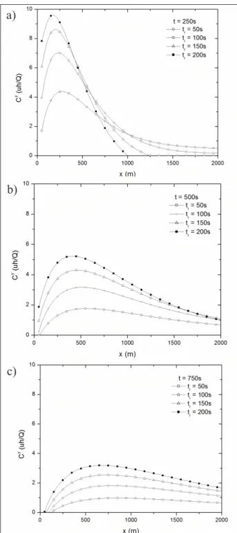
Figure 4 shows the nondimensional ground level concentration (Cyuh / Q) as a function of the source distance with variable duration releases (t_r= 50, 100, 150, 200 seconds) for three different times (t = 250, 500 and 750 seconds), emitted through a stack with a physical height of 10 m, in micrometeorological conditions characterized by a 2 m/s wind velocity, a 1,100 m mixing layer, w_* = 2 m/s and L = -10 m.

Figure 4 shows that the concentration peak values increases as the duration of the release grows longer, until it reaches

a limit value, for suficiently long durations of the release.

Besides, the concentration peak values decrease with the source distance increase.

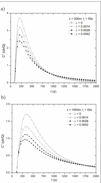
Figure 5 demonstrates the concentration time evolutions with the parameters of the reference situation for time release of 50 seconds to different values of the

chemical-physical decay coeficient (λ), at downwind distance of 500 and 1000 m (typical values of λ: 10-6 to 10-2_{). It also shows that the concentration peak} values decrease as the downwind distance increase.

!

!

!

a)

b)

c)

Figure 4: Crosswind integrated concentration as a function of the source distance for three different times (t = 250, 500 and 750 seconds) and different durations of release (t_r = 50, 100, 150 and 200 seconds).

Also, as the downwind distance increase, the peak position changes with respect to time and the peak concentration variation between the chemical-physical decay constants increase.

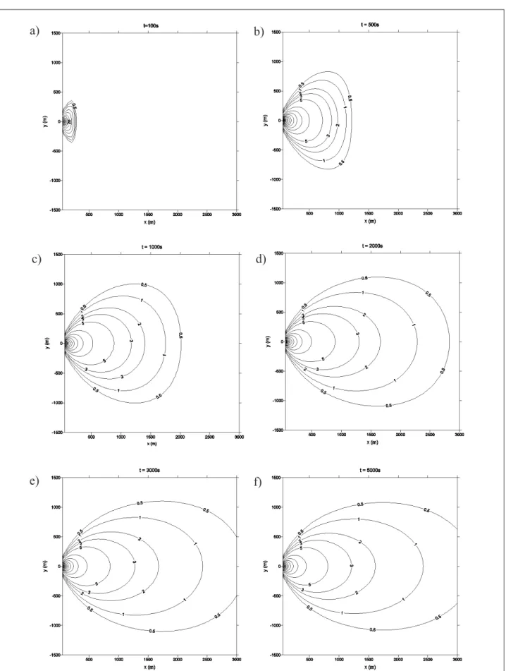
Figure 6 has the concentration distributions in the horizontal xy-plane at ground-level for six different

times: t = 100, 500, 100, 2000, 3000 and 5000 seconds.

These isolines of equal concentration corresponds to the solution t_r > t.

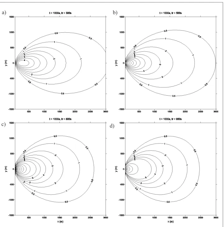
As expected, when time becomes longer, the concentrations values enter into a steady-state condition. Figure 7 shows concentration distributions in the horizontal xy-plane at ground-level for the time t = 1000 seconds and four different time release (t_r = 300, 500,

800 and 950 seconds). The lines represent isolines of equal concentration.

As the duration of the release becomes longer, the concentrations values enter into a steady-state condition. Comparing Fig. 6 for t = 1000 seconds with Fig. 7, this

afirmative is clearly observed.

Furthermore, due to lack of experimental data with rockets, we evaluated the performance of the model (t_r > t, with a single source at 115 m) with the boundary layer parameterization proposed, using the well-known Copenhagen data set (Gryning et al., 1987). The Copenhagen data set is composed of tracer SF₆ data from dispersion experiments carried out in Northern Copenhagen. The tracer was released without buoyancy from a tower at 115 m height, and was collected at ground-level positions in up to three crosswind arcs of tracer sampling units. The sampling units were positioned from 2 to 6 km far from the point of release. We used the values of the crosswind integrated concentrations normalized with the tracer release rate from Gryning et al. (1987). Tracer releases typically start up one hour before the tracer sampling and stop at the end of the sampling period. The site was mainly residential with a roughness length of 0.6 m. Generally, the distributed data set contains hourly mean values of concentrations and meteorological data. However, in this work, data with a greater time resolution were used. In particular, 20 minutes averaged measured concentrations and 10 minutes averaged values for meteorological data were used. In such manner, in the present work, the variables (L, u_* ,

w*) in the Copenhagen data set are dynamical (except

the variable h). For details of the experimental data, see the work of Tirabassi and Rizza (1997).

The results obtained with the model are compared with the M4PUFF model (Tirabassi and Rizza, 1997), which is based on a general technique for solving the K-equation using the truncated Gram-Charlier expansion (type A)

of the concentration ield, and a inite set equation for

the corresponding moments. Table 1 presents some performance measurements, obtained using the well-known statistical evaluation procedure described by Hanna (1989). The statistical index FB indicates whether the predicted quantities underestimate or overestimate the observed ones. The statistical index NMSE represents the quadratic error of the predicted quantities in relation to the observed ones. The best results are indicated by values nearest 0 in NMSE, FB, and FS, and nearest 1 in COR and FA2.

The statistical indices point out that a good agreement is obtained between experimental data and the model.

!

!

a)

Figure 6:Concentrations distributions in the horizontal xy-plane at ground-level for six different times: t = 100, 500, 100, 2000, 3000 and 5000 seconds, for the solution t_r > t.

!

!

!

!

!

!

a)

b)

c)

d)

A more detailed inspection of the Table 1 can stress that the model does a very well simulation of the observed concentrations presenting the best values for NMSE, COR (81%), and FA2 (95%).

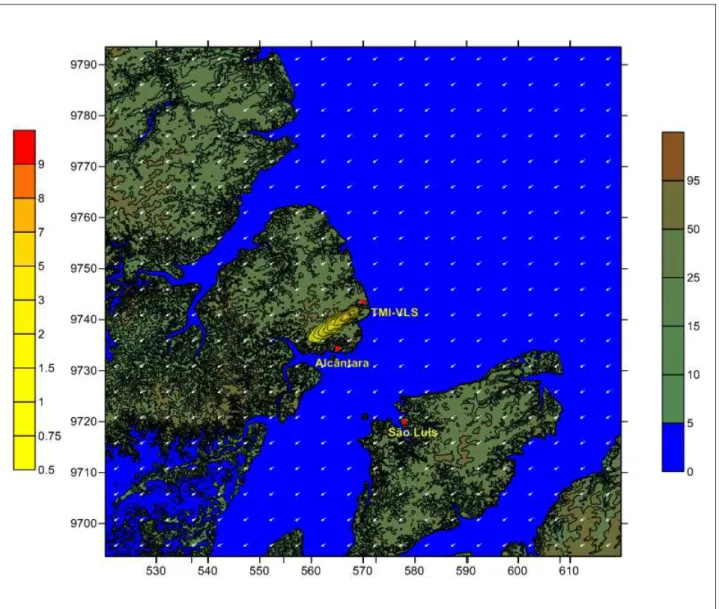
Finally, a simulation considering a grid of 100 x 100 km in the region covered by the Alcântara Launch Center is carried out. The main points are shown in Fig. 8, with the vector wind speed and dispersion of the plume. The concentration unit is ppm.

CONCLUSIONS

A solution of the time-dependent advection-diffusion equation in the construction of the MSDEF has been

Figure 7:Concentrations distributions in the horizontal xy-plane at ground-level for t = 1,000 seconds and four different times releases: t_r = 300, 500, 800 and 950 seconds, for the solution t > t_r.

!

!

!

!

a)

b)

c)

_d)

Table 1: Statistical evaluation of model results (Copenhagen dataset)

Model NMSE R FA2 FB FS

MSDEF 0.15 0.81 0.95 0.18 0.38

presented. This solution considers duration time release, chemical-physical decay, settling velocity, scavenging coefficient, and can be applied for describing the turbulent dispersion of many scale quantities, such as air pollution, radioactive material, heat, and so on. From the previous results, we promptly notice the aptness this model to understand the time evolution of the concentration and its dependency on the duration of the contaminant emission. In fact, this model allows us to simulate the continuous, short-term, and instantaneous emissions. In particular, the model is suitable for an initial and rapid assessment of atmospheric dispersion under emergency conditions without sophisticated computing resources. The model can be used in different conditions of atmospheric stability, making it possible to predict or simulate the concentration in accordance with emergency plans and pre and post-launches for environmental management,

in situations of rocket launches in the Alcântara Launch Center.

To show the solution performances in actual scenarios, a parameterization of the ABL has been introduced, and their values have been compared with experiment dataset. The analysis of the results shows a reasonably good agreement between the computed values and the experimental ones. The discrepancies with the experimental data depend not on the solution of the advection-diffusion equation but on the equation itself, which it is only a reality model. Moreover, a source of discrepancies between the predicted and measured values lies in the ABL parameterization used (i.e., vertical wind and eddy diffusivity profiles). Although models are sophisticated instruments that ultimately reflect the current state of knowledge on turbulent transport in the atmosphere, the results they provide

!

are subject to a considerable margin of error. This is due to various factors, including the uncertainty of the atmosphere intrinsic variability. Models, in fact, provide values expressed as an average, that is, a mean value obtained by the repeated performance of many experiments, whereas the measured concentrations are a single value of the sample to which the ensemble average provided by models refers.

This is a general characteristic of the theory of atmospheric turbulence and is a consequence of the statistical approach used in attempting to parameterize the chaotic character of the measured data. In light of the considerations, an analytical solution is useful to evaluate the performances of sophisticated numerical dispersion models, which numerically solve the advection-diffusion equation, yielding results that can be compared not only with experimental data but, in an easy way, with the solution itself, to check numerical errors without the uncertainties presented above.

ACKOWLEDGEMENTS

The authors thank the Brazilian National Council for

Scientiic and Technological Development (CNPq) for the partial inancial support of this work through their

Research Grant (PQ).

REFERENCES

Abate, J., Valkó, P.P., 2004, “Multi-precision Laplace transform inversion”, International Journal for Numerical Methods in Engineering, Vol. 60, pp. 979-993. doi: 10.1002/nme.995

Bianconi, R., Tamponi, M., 1993, “A mathematical model of diffusion from a steady source of short duration in a

inite mixing layer”, Atmospheric Environment, Vol. 27,

No. 5, pp. 781-792. doi:10.1016/0960-1686(93)90196-6

Bjorklund, J.R., Dumbauld, J.K, Cheney, C.S. and Geary, H.V., 1982, “User’s manual for the REEDM (Rocket

Exhaust Efluent Diffusion Model) compute program”,

NASA contractor report 3646. NASA George C. Marshall Space Flight Center, Huntsville, AL.

Bjorklund, J.R., 1990, “User instructions for the Real-Time Volume Source Dispersion Model (RTVSM)”, H.E Cramer Company, Inc. Report TR-90-374-02, prepared for U.S. Army Dugway Proving Ground, Dugway, UT.

Bjorklund, J.R., Bowers, J.F., Dodd, G.C. and White, J.M., 1998, “Open Burn/Open Detonation Dispersion Model (OBODM) users’ guide”, Vol. 2, Technical description.

West desert test center, US Army Dugway proving ground, Dugway, Utah.

Briggs, G.A., 1975, “Plume Rise Predictions, Lectures on Air Pollution and Environmental Impact Analyses”, D.A. Haugen ed., American Meteorological Society, Boston, MA, pp. 59-111.

Degrazia, G.A., Campos Velho, H.F. and Carvalho, J.C., 1997,

“Nonlocal exchange coeficients for the convective boundary

layer derived from spectral properties”, Contributions to Atmospheric Physics, Vol. 70, No. 1, pp. 57-64.

Degrazia, G.A., Mangia, C. and Rizza U., 1998, “A comparison between different methods to estimate the lateral dispersion parameter under convective conditions”, Journal of Applied Meteorology, Vol. 37, pp. 227-231.

Dumbauld, R.K., Bjorklund, J.R. and Bowers, J.F., 1973, “NASA/MSFC multilayer diffusion models and computer program for operational prediction of toxic fuel hazards”, NASA Contractor Report CR-129006, NASA George C. Marshall Space Flight Center, Huntsville, AL.

EPA-454/B-03-002, 2004. User’s Guide for the AERMOD meteorological preprocessor (AERMET).

Gryning, S., Holtslag, A., Irwing, J. and Silversten, B., 1987, “Applied dispersion modeling based on

meteorological scaling parameters”, Atmospheric

Environment, Vol. 21, pp. 79-89.

Hanna, S.R., 1989, “Conidence limit for air quality

models as estimated by bootstrap and jacknife resampling methods”, Atmospheric Environment, Vol. 23, pp. 1385-1395.

Hφjstrup, J., 1982, “Velocity spectra in the unstable boundary layer”, Journal of Atmospheric Science, Vol. 39, pp. 2239-2248.

Huang, C.H., 1979, “A theory of dispersion in turbulent shear

low”, Atmospheric Environment, Vol. 13, pp. 453-461.

Mangia, C., Moreira, D.M., Schipa, I., Degrazia, G.A., Tirabassi, T. and Rizza, U., 2002, “Evaluation of a new eddy diffusivity parameterisation from turbulent Eulerian spectra in different stability conditions”, Atmospheric Environment, Vol. 36, pp. 67-76.

Moreira, D.M., Rizza, U., Vilhena, M.T. and Goulart, A.G., 2005a, “Semi-analytical model for pollution dispersion in the planetary boundary layer”, Atmospheric Environment, Vol. 39, No. 14, pp. 2689-2697.

Moreira, D.M, Carvalho, J.C., Goulart, A.G. and Tirabassi, T., 2005b, “Simulation of the dispersion of pollutants using two approaches for the case of a low source in the SBL: evaluation of turbulence parameterisations”, Water, Air and Soil Pollution, Vol. 161, pp. 285-297.

Moreira, D.M, Ferreira Neto, P.V. and Carvalho, J.C., 2005c, “Analytical solution of the Eulerian dispersion equation for nonstationary conditions: development and evaluation”, Environmental Modelling and Software, Vol. 20, No. 9, pp. 1159-1165.

Moreira, D.M., Tirabassi, T. and Carvalho, J.C., 2005d, “Plume dispersion simulation in low wind conditions in stable and convective boundary layers”, Atmospheric Environment, Vol. 39, No. 20, pp. 3643-3650.

Moreira, D.M, Vilhena, M.T., Tirabassi, T., Costa, C. and Bodmann, B., 2006, “Simulation of pollutant dispersion

in the atmosphere by the Laplace transform: the ADMM approach”, Water, Air and Soil Pollution, Vol. 177, pp. 411-439.

Moreira, D.M., Trindade, L., 2010, “Manual do Usuário do Modelo MSDEF (Modelo Simulador da Dispersão

de Eluentes de Foguetes)”, Versão 1.0/2010, Relatório

Técnico, CTA/IAE/ACA. 70pp.

Nyman, R.L., 2009, “NASA Report: Evaluation of Taurus II Static Test Firing and Normal Launch Rocket Plume Emissions”.

Stephens, J.B., Stewart, R.B., 1977, “Rocket exhaust

efluent modeling for thopospheric air quality and

environmental assessment”, National Aeronautics and Space Administration – NASA Technical Report.

Stroud, A.H., Secrest, D., 1966, “Gaussian Quadrature Formulas”, Englewood Cliffs, N.J., Prentice Hall, Inc.