ABSTRACT: The Operational Modal Analysis technique is a methodology very often applied for the identiication of dynamic systems when the input signal is unknown. The applied methodology is based on a technique to estimate the Frequency Response Functions and extract the modal parameters using only the structural dynamic response data, without assuming the knowledge of the excitation forces. Such approach is an adequate way for measuring the aircraft aeroelastic response due to random input, like atmospheric turbulence. The in-light structural response has been measured by accelerometers distributed along the aircraft wings, fuselage and empennages. The Enhanced Frequency Domain Decomposition technique was chosen to identify the airframe dynamic parameters. This technique is based on the hypothesis that the system is randomly excited with a broadband spectrum with almost constant power spectral density. The system identiication procedure is based on the Single Value Decomposition of the power spectral densities of system output signals, estimated by the usual Fast Fourier Transform method. This procedure has been applied to different light conditions to evaluate the modal parameters and the aeroelastic stability trends of the airframe under investigation. The experimental results obtained by this methodology were compared with the predicted results supplied by aeroelastic numerical models in order to check the consistency of the proposed output-only methodology. The objective of this paper is to compare in-light measured aeroelastic damping against the corresponding parameters computed from numerical aeroelastic models. Different aerodynamic modeling approaches should be investigated such as the use of source panel body models, cruciform and lat plate projection. As a result of this investigation it is expected the choice of the better aeroelastic modeling and Operational Modal Analysis techniques to be included in a standard aeroelastic certiication process.
KEYWORDS: Operational modal analysis, In-light aeroelastic testing, Model correlation.
Comparison of In-Flight Measured and Computed
Aeroelastic Damping: Modal Identiication
Procedures and Modeling Approaches
Roberto da Cunha Follador1, Carlos Eduardo de Souza2, Adolfo Gomes Marto3, Roberto Gil Annes da Silva4,
Luis Carlos Sandoval Góes4
INTRODUCTION
BACKGROUNDAeroelastic light testing is associated frequently to lutter testing, deined as an experimental way to predict aeroelastic stability margins from measured aeroelastic damping. he light test community routinely spends considerable time and money for envelope expansion of aircrat with new systems installed. A method to safely and accurately predict the speed associated to aeroelastic instabilities onset such as lutter could greatly reduce these costs.
Several methods have been developed with that goal. hese methods include approaches based on extrapolating damping trends from available aeroelastic damping and assuming data extrapolation (Kehoe 1995). All of these approaches lead to a prediction of lutter speed from subcritical conditions. here are a number of lutter prediction methodologies available in the literature. Dimitriadis and Cooper (2001) and Lind and Brenner (2002) present comparisons between most of the known lutter prediction methodologies. hese references are good texts for understanding some lutter testing techniques to be commented next.
he classical lutter prediction methodologies include, for example, Zimmerman and Weissenburger (1964) approach. he lutter margin concept was introduced, based on the investigation of the two degrees of freedom typical section aeroelastic stability, based on Pines (1958) aerodynamic simpliication. Even assuming steady-state aerodynamics, it was possible to develop lutter margin equation, function of measured aeroelastic damping
doi: 10.5028/jatm.v8i2.558
1.Departamento de Ciência e Tecnologia Aeroespacial – Instituto de Estudos Avançados – Direção – São José dos Campos/SP – Brazil. 2.Universidade Federal de Santa Maria – Centro de Tecnologia- Departamento de Engenharia Mecânica – Santa Maria/RS – Brazil. 3.Departamento de Ciência e Tecnologia Aeroespacial – Instituto de Aeronáutica e Espaço – Divisão de Aerodinâmica – São José dos Campos/SP – Brazil. 4.Departamento de Ciência e Tecnologia Aeroespacial – Instituto Tecnológico de Aeronáutica – Divisão de Engenharia Aeronáutica – São José dos Campos/SP – Brazil.
Author for correspondence: Roberto Gil Annes da Silva | Departamento de Ciência e Tecnologia Aeroespacial – Instituto Tecnológico de Aeronáutica – Divisão de Engenharia Aeronáutica | Praça Marechal Eduardo Gomes, 50 – Vila das Acácias | CEP: 12.228-900 – São José dos Campos/SP – Brazil | Email: [email protected]
and frequency at the same time. This approach presumes information not only from measured aeroelastic damping, but also the measured aeroelastic frequency evolution as a function of dynamic pressure. It can be understood as a safer way to extrapolate the measured aeroelastic information (frequency and damping) for estimating the lutter dynamic pressure.
After Zimmerman and Weissenburger (1964) researches several authors have been developing safer ways for experimental flutter predictions. Methods such as the Lind and Brenner “Flutterometer” are another tool that predicts flutter from experiments (Lind and Brenner 2000). It is also a model-based approach, but not in the same sense of Zimmerman-Weissenburger flutter margin method, which is based on typical section equations. Basically, the Flutterometer uses both flight data represented as frequency domain transfer functions and theoretical models to predict the onset of flutter. This method works like a measurement instrument, as suggested by its name. A robust flutter speed is computed at every test point. The initial step is to compute an uncertainty description for the model at that flight condition. With this uncertainty model it is possible to compute the robust flutter speed, based on the application of µ-method on a theoretical model which includes now uncertainty variations. This method can be understood as safer because it computes flutter speeds based on updated theoretical model, which takes into account flight test data. The envelope function method is another data-based approach, besides the classical damping extrapolation method (Cooper et al. 1993). However it predicts the onset of lutter based entirely on the analysis of time-domain measurements from sensors in response to an in-light impulse excitation. It might be suitable for flight testing using pyrotechnical thrusters, also known as “bonkers”, for example. he nature of this method is similar to a damping extrapolation based approach. he only diference is that the envelope function method does not estimate modal damping. he time domain aeroelastic response envelope indicates the loss of damping as far as a slower output signal decay rate is observed. hus, the shape of the time response plots can be used to indicate a loss of damping, in other words, lutter.
Most of flight testing methodologies presented above presume excitation forces from any kind of artiicial input, such as vanes, pyrotechnical thrusters and inertial rotating systems, for example. An input signal is known and, in most of the cases, from a frequency to response output to input relation, it is
possible to identify a dynamic aeroelastic system. he natural consequence of such an approach is the need to introduce a device for the aircrat excitation during light. Furthermore, this device represents costs (operation/royalties, maintenance/ support, and acquisition) and structural dynamic changes in the airframe under investigation. It also requires light test hours for calibration, manpower for installation and removal ater tests. Recently, a cooperative program (Silva et al. 2005) involving several research centers, including universities and defense agencies, has been established. It looks for safer and cheaper light testing methodologies focused on the development of improved procedures for lutter tests. hese tests involve aircrat operation at hazardous light conditions. he risk minimization comes from prior numerical model analyses and also by extrapolation of subcritical damping measurements. Among the commented objectives of these collaborative activities, the development of reliable procedures for lutter prediction methods is relevant. hese procedures may allow larger speed increments during light test for reducing test points, without compromising the safety.
OPERATIONAL MODAL ANALYSIS
he present investigation intends to report some experiences for computing aeroelastic damping trends as a function of light speed, based on an output-only modal parameter extraction technique, known as Operational Modal Analysis (OMA), which presumes a modal parameters identiication methodology only from system dynamic response measurements. he determination of parameters using OMA as an aeroelastic modal analysis tool allows observing the dynamic behavior of the structure of interest embedded in its original operating conditions. Moreover, the inclusion of artiicial excitation systems is not necessary. Input excitations can be considered as continuously generated, such as the disturbances present in atmospheric light environment (random atmospheric turbulence), or even engine-generated vibrations. Most of the airframe vibration modes can be excited by these kinds of input, and, consequently, these modes can be identiied representing the aeroelastic modal characteristics at known Mach number and light altitude.
165
Comparison of In-Flight Measured and Computed Aeroelastic Damping: Modal Identiication Procedures and Modeling Approaches
the objective of the technique was the use of data acquired during non-speciic aeroelastic testing, thus eliminating the need of a speciic campaign for lutter investigation. he YF-16 aircrat aeroelastic clearance, for example, was also based on random atmospheric excitation as an input source for in-light dynamic response measurements.
Otherwise, the main disadvantage (Kehoe 1995) is the lower excitation capability of atmospheric turbulence, when compared to a sine sweep input driven by an excitation aerodynamic vane, for example. Only a few of low-frequency mode shapes could be identiied, since there is not suicient force strength to excite the airframe. his limitation directly impacts on the data reduction quality, since the signal-to-noise ratio is oten low. Another disadvantage is the need of long data records to obtain results with a suicient conidence level. However, at that time, data recording could be a limiting issue. Today computational resources allow huge databases structuring and recording, at near real time speeds.
Even considering the drawbacks presented by Kehoe (1995), a number of applications of output-only modal analysis methods to system modal parameter identiication have been developed. Brincker et al. (2001) presented a frequency domain OMA technique named as Frequency Domain Decomposition (FDD) for the modal identiication of output-only systems. he modal parameters were estimated by simple peak picking approach. However, by introducing a decomposition of the spectral density function matrix, the response spectra can be separated into a set of single degree of freedom systems, each corresponding to an individual mode. Close modes can be identiied with high accuracy even in the case of strong noise contamination of the signals. he same OMA/FDD techniques are well documented in the theses of Verboven (2002), Cauberghe (2004) and Borges (2006).
Peeters et al. (2006) presented modern frequency-domain modal parameter estimation methods applied to in-flight aeroelastic response data measurements of a large aircrat. Data acquired from applied sine sweep excitation and natural turbulence excitations were available during short-time periods. he authors observed that the same modes could be extracted even by applying OMA to the turbulence spectra or by classical modal analysis applied to the sweep Frequency Response Functions (FRFs). In this reference a non-parametric FRF estimation method was also applied, which overcomes the typical tradeof between leakage and noise when processing random or single sweep data. Despite the fact that the damping ratios
are very critical parameters for lutter analysis, it was observed that rather large uncertainties are associated with this modal parameter. Depending on the data pre-processing, parameter estimation method and the used data (sweep versus turbulence), relatively large diferences in damping ratios were found.
Differently from traditional frequency domain OMA methods, Uhl et al. (2007) presented an idea of lutter margin detection algorithm which is based on identiication of natural frequencies and modal damping ratio for airplane structure employing in-light vibration measurements. he method is based on application of wavelets iltering for decomposition of measured system response into components related to particular vibration modes. In the second step classical Recursive Least Square (RLS) estimation methods are used to obtain Autoregressive Moving Average (ARMA) model parameters. he results of modal parameters tracking, using designed real-time embedded systems, were compared with more classical in-light modal analysis at discrete light points.
Within the perspective extracted from previous investigation on OMA, this paper aims to continue the investigation reported by Ferreira et al. (2008). he present study considered OMA as a tool for identifying the modal behavior of an aircrat modiied by the addition of new systems such as external stores. As a irst step, data measurements from an in-light aeroelastic testing using pyrotechnical thrusters were used for the application of FDD/OMA method (Silva et al. 1999). Ater analyzing this irst data set (Ferreira 2007), it was concluded that special recommendations are necessary for the best output to noise statistical relation. he scope of the present investigation is to include improvements on testing of an output-only frequency domain modal analysis procedure, based on measured data from resident instrumentation during operational light conditions. Follador (2009) includes a diferent data acquisition approach, extending data acquisition time frame for improving the lack of statistical contents of the data acquired in the 1999’s lutter testing lights.
considered a good alternative for aeroelastic model correlation/ update, especially at conditions where the unsteady aerodynamic modeling lacks on representing non-linear efects.
Comments on light tests techniques are also presented, regarding relevant aspects related to mission planning, especially in relation to the concerns of the teams involved in the correct sizing of the test needs. he detailed methodology describes the test platform, Data Acquisition System (DAS) and tests performed. Details of instrumentation, sensors positioning, data acquisition time interval and test points planning are also presented. he steps for the collected data processing as well as procedures used in conducting the reduction through the use of Brüel & Kjaer (B&K) OMA®sotware are detailed. Comparisons between results obtained in this study and those obtained by Ferreira (2007), who used the same methodology but with diferent input signal source, are performed. In the study conclusions, there are comments on the feasibility of using the proposed methodology for operational modal analysis applied to the identiication of aircrat modal parameters in light. Further comments include contributing factors for correct identiication of aeroelastic modal data, with emphasis on the application processes for aeroelastic testing implementation suggesting actions for future research.
THEORETICAL BACKGROUND
NUMERICAL AEROELASTIC MODELhe aircrat aeroelastic behavior was studied in order to obtain a theoretical database for comparison. he structure of the aircrat was modeled with Finite Elements Method (FEM) as equivalent beams. he dynamic parameters (natural frequencies and mode shapes) calculated through the FEM model have been updated based on modal parameters from Experimental Modal Analysis (EMA) obtained from a Ground Vibration Test (GVT). he experimental structural modal damping was not incorporated to the FEM model.
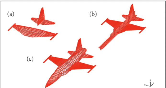
The unsteady aerodynamic model is a finite element potential aerodynamic solution, implemented in ZAERO sotware system, named as ZONA 6 method. Diferent modeling approaches were used for understanding the sensitivity in terms of aeroelastic stability behavior. Flat plate only, cruciform and body aerodynamic models were generated to identify the aeroelastic coupling mechanisms. Figure 1 shows the three aerodynamic models as described. References comprise the unsteady aerodynamics theoretical foundations such as modeling
techniques including the procedure for aeroelastic stability analysis, known as g-method (ZONA Technology 2007).
he aeroelastic analysis shall be conducted for selected conigurations and light conditions. Computed frequency and aeroelastic damping are plotted as a function of Mach number or true airspeed, if a given light level is assumed.
EXPERIMENTAL MODAL ANALYSIS
he EMA aims to estimate modal characteristics, establishing direct relations between the outputs and inputs signals observed in the system under analysis. Considering a dynamic system represented by a multiple degrees of freedom equation of motion as:
Figure 1. Flat plate (a), cruciform (b) and body aerodynamic models (c).
x y
z
when transformed to the frequency domain using a Laplace Transform, this equation can be written in terms of Laplace variable s as:
where: M is the mass matrix; C is the damping matrix; K is the stifness matrix; X is the state variables vector; F is an external force.
By deinition, the transfer function matrix [H(s)] determines the input/output relation:
his transfer function matrix can be expressed in terms of poles λr and residues Rr and their conjugated λr and Rr as in
(a) (b)
(c)
(1)
(2)
167
Comparison of In-Flight Measured and Computed Aeroelastic Damping: Modal Identiication Procedures and Modeling Approaches
Maia et al. (1997): the statistical behavior of signals. here are several methods in time domain or frequency domain used to estimate the modal characteristic when input signals are known. Maia et al. (1997) show in details some of these methods, such as the time domain Least-Squares Complex Exponential Method (LSCE) and the frequency domain Rational Fractional Polynomial Method (RFP).
OPERATIONAL MODAL ANALYSIS
The methodology for using OMA as a system modal parameter identiication tool consists in carrying out lights of an instrumented aircraft for measuring accelerations at diferent points on the aircrat structure. Once the aeroelastic response is measured, the determination of modal parameters can be performed.
OMA can also be performed even as a frequency or a time domain method. Examples of time domain methods are the Autoregressive Moving Average Method (ARMAV) and the Stochastic Subspace Identiication (SSI). he frequency domain examples are: the Basic Frequency Domain method (BFD), the FDD method and the Enhanced Frequency Domain Decomposition method (EFDD). The latter is assumed in the present methodology. his method allows identiication of frequencies, damping ratio and the corresponding mode shapes from the aeroelastic system. It assumes that the input signal, the atmospheric disturbance, is random, stationary and ergodic, i.e. the statistical properties (mean, standard deviation, variance etc.) are time-invariant.
Combining the FRFs using H1 estimator as expressed in Eq. 6 with the same FRFs using H2 we can have an output/input spectrum relationship as:
where: Rr = Pr ∙ Qr ∙ {Ψr} ∙ {Ψr}T, Pr and Qr are constants dependent on the poles and {Ψr} is the vector proportional to the modal shape.
Evaluating the transfer function only in frequency domain, i.e.s = jω (j is the complex number), the FRF matrix can be expressed as:
he FRFs can be extracted from traditional measurements system by an H1(ω) estimator, which minimizes the noise on the output using Sfx (ω) output cross spectrum and input-input spectrum Sf (ω):
he H2 estimator is the other way to extract the FRFs. his estimator minimizes the noise on the input using the input autospectrum Sxx (ω) and input-output cross spectrum Sxf (ω):
As described in Bendat and Pierson (1980), the Saa (ω) autospectrum is related to Raa (ω) autocorrelation by a Fourier transform:
where: τ is the time.
In same way the cross-spectrum Sac (ω relates with cross-correlation of signals Rac (ω):
he spectrum and correlation give us knowledge about
Assuming the turbulence disturbance as white noise, the input autospectrum can be considered as a constant matrix [S]. his approach is appropriated for aeroelastic analysis in the frequency range between 0 and 100 Hz, as we can see, for example, in Hoblit (1988) and in Eichenbaum (1972). herefore, the autospectrum can be expressed as a function of residues and the corresponding poles:
(4)
(5)
(6)
(7)
(10)
(11) (8)
(9)
where: superscript H represents the complex conjugate; Rk represent the residues and λk, the poles.
hroughout an expansion in partial fractions, we have:
and
where: [Ak] and [Bk] are the residues matrices of the system output power spectral density.
Similarly, as presented in the theory for EMA, it can be shown that the residues are proportional to the vibrating modes of a slightly damped structure (Borges 2006):
where: dk is a diagonal matrix operator.
Replacing it in the expression on Eq. 4, we have:
For a given frequency ω, only a few modes contribute signiicantly to the residue. his allows us to determine the number of modes of interest, denoting this set of modes by Sub(ω). hus, it is possible to rewrite the Matrix Output Power Spectral Density about the modes of interest. his matrix is composed by autospectrum Sii of each output and cross-spectrum Cij among each one, as shown in Batel (2002):
he size of this matrix is N ×N , for each jω, with N being the number of output measurement sensors and jω a given discrete frequency line.
he autospectrum Sii and cross-spectrum Cij can be extracted from measured signals applying the Fast Fourier Transform (FFT) in M sample windowing:
where: Xiand Xjare the FFT of each window.
The spectrum estimation accuracy will depend on the time windowing and the numbers of windows. his statistical character will deine the total acquisition time for the light test. Each window time needs to be long enough to yield a suicient frequency resolution in order to estimate the damping factor. he output power spectral density matrix Sxx has discrete points in frequency. For each frequency line the square matrix can be decomposed into singular values Siand associated vectors Ui from the application of a Singular Value Decomposition:
his technique reduces the Sxx matrix to a more simpliied (or canonical) form that contains singular values for each line. For a given x = i or y = j, for example, when Sijoutput power spectral density matrix is analyzed in this form, the peak amplitudes of [Si] are associated to dominant natural modes, as described in Eq. 14.
One way to estimate the damping factor for each mode identified by peak-peaking is the investigation of the associated vector. This is the improvement of the Peak-Peaking method described in Maia et al. (1997). The EFDD uses the Modal Assurance Criterion (MAC) in order to correlate the chosen modes with associated modes in a previous and a posterior frequency line:
To the largest MAC value of a given chosen vector, there are many corresponding singular values proportional to the SDOF Spectral Bell function. Disconsidering uncorrelated vectors and applying the IFFT on the Spectral Bell function, it is possible to estimate the autocorrelation of this signal using Eq. 8.
Once identified the system autocorrelation function, corresponding to a single degree of freedom mode, the ratio of damping is determined using the concept of logarithmic decrement obtained by a linear regression, as seen previously for systems of one degree of freedom in Ewins (1986): (12)
(13) (17)
(14)
(15) (18)
(16)
(16)
j (ω)
169
Comparison of In-Flight Measured and Computed Aeroelastic Damping: Modal Identii cation Procedures and Modeling Approaches
where: r0 is the initial value of the autocorrelation function; rkis the k-th extreme.
h erefore, the damping factor can be obtained from the logarithmic decrement:
THE TEST POINT PREPARATION
Data collection was planned for a clean aircrat coni guration at Mach numbers ranging from 0.7 to 0.95, with a 0.05 Mach increment, at 1,000 m above sea level. h e altitude was hold approximately constant, in order to maintain a constant air density. The tolerance ranges for Mach and altitude were ± 0.01 and ± 100 m, respectively.
According to recommendations (Ferreira 2007), at least 50 samples of 2 s each were chosen, in order to statistically extract the accurate spectrum with frequency resolution enough to capture the damping factor (see Eq. 16). h is choice has dei ned the time range stabilization on each measured test point.
DATA COLLECTION SYSTEM
h e accelerations could be recorded along a known time period. h e accelerometer DAS basic architecture is composed of a programmable DAS (KAM-500). A high-speed and compact l ash memory module with a capacity of 2 GB of memory was used for storing recorded data. h e technology of solid-state data recording allowed a rapid extraction of data from l ight tests just at er the aircrat landing.
h e accelerometers used for data acquisition were of piezo-resistive type (3140 model — ICSensors), with low-frequency band response (0 – 200 Hz) with ± 20 m/s2 amplitude range. h e sensor positioning is presented in Fig. 2, including a reference number and axis alignment, namely the vertical axis (z axis) or lateral (y axis) in datum reference frame. h e determination of the positions was made in order to take into account relevant and the corresponding natural frequency can be obtained as:
where: d means damped natural frequency and n rel ects the undamped natural frequency.
FLIGHT TEST AND ANALYSIS
PROCEDURES
Based on information from a theoretical model, the l ight test planning was conducted applying the concept of gradual approximation to a more critical flight condition. Following this doctrine, all flight testing start at the most conservative situation. Aircraft response is measured and compared with theoretical model predictions. This is the flight stage under investigation reported in the present paper.
Several techniques for in-flight tests require that the pilot himself keep a number of parameters monitored. Nowadays these parameters can be directly registered by the DAS or be monitored by telemetry for all flight duration. However, the stabilization of some parameters is necessary in order to compare the experimental analysis and the numerical ones. The time required to achieve stability around a steady flight condition is a function of response time of those parameters.
An important issue that must be dealt with using the OMA as an in-flight parameter identification tool is assuming the hypothesis that the atmospheric turbu-lence could be modeled as a continuous white noise, as
discussed earlier. Figure 2. Accelerometers positioning in the airframe. 15y
z
y x
x x
x
x xx
x x
x x
x x x
x x 7z
5z 10y
14y13z 4z
3z
1z 2z
9z
11z 12y 6z
8z x (19)
(20)
aeroelastic information such as structural mode shapes and frequencies. A representative and simpliied model has been assembled and inserted in the signal processing sotware in order to verify the relationship between the identiied natural vibration mode and theoretical predications.
he measured data (accelerations as a function of time) was converted to universal ile format in order to be processed by the B&K OMA® sotware. Using this sotware, the PSD matrix of each signal was calculated, following Bendat and Pierson (1980) recommendations. The hanning window was used with an overlap of 66%. Four seconds for each window were considered, which allowed a frequency resolution of 0.25 Hz. he purpose of the windowing is to prevent the occurrence of leakage phenomenon, to prevent the identiication of non-physical peaks in power spectrum density plots, and enable the correct implementation of the Fourier Transform over the output signal (Avitabile 2001).
he EFDD was applied for each PSD matrix correspondent to each light condition. he mode shapes are identiied over the Single Value Decomposition (SVD) curves that are correlated using MAC algorithm cited in Eq. 18. he autocorrelations were calculated with IFFT. he damping ratio factor ξr and natural frequency ωr were calculated based on the best exponential range of the autocorrelation correspondent to each mode shape identiied. Ater computing these modal parameters, extracted from the lutter light test, they were compared with the same parameters estimated from the aeroelastic analysis.
RESULTS
THEORETICAL AEROELASTIC ANALYSIS RESULTS
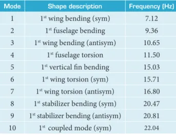
he results of the present investigation are divided into theoretical aeroelastic analysis results and in-light operational modal analysis results. he theoretical model described aims at representing the aircrat in the coniguration to be tested. he dynamic analysis results are summarized in Table 1 which shows the irst ten natural frequencies identiied from the structural dynamic analysis of the airframe. he selected mode shapes include symmetrical and antisymmetrical liting surfaces modal displacements. Figure 3 presents the irst ten structural mode shapes plots, interpolated to the doublet/body source panels aerodynamic mesh.
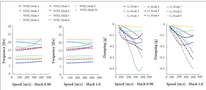
A non-matched lutter analysis was performed to observe the evolution of aeroelastic damping and frequencies as a function of airspeed and even to understand possible coupling
Mode Shape description Frequency (Hz)
1 1st wing bending (sym) 7.12
2 1st fuselage bending 9.36
3 1st wing bending (antisym) 10.65
4 1st fuselage torsion 11.50
5 1st vertical in bending 15.03
6 1st wing torsion (sym) 15.71
7 1st wing torsion (antisym) 16.80
8 1st stabilizer bending (sym) 20.47
9 1st stabilizer bending (antisym) 20.81
10 1st coupled mode (sym) 22.04
Table 1. Aircraft natural frequencies for the irst ten modes.
Sym: Symmetrical; antisym: Antisymmetrical.
Figure 3. Selected aircraft mode shapes for aeroelastic investigation.
Mode 1
Mode 2
Mode 3
Mode 5 Mode 4
Mode 6
Mode 7
Mode 8
171
Comparison of In-Flight Measured and Computed Aeroelastic Damping: Modal Identiication Procedures and Modeling Approaches
mechanisms. It was fixed a constant flight level setting a constant density. The g-method for aeroelastic stability analysis was employed for each reference Mach number. he results are summarized in Figs. 4 and 5. It was not considered structural damping since the FEM model does not include such material properties.
However, the true aeroelastic damping solution for a given Mach number, considering the g-method damping valid for subcritical aeroelastic conditions, is obtained as a matched point lutter analysis. For each Mach number, the corresponding
aeroelastic damping and frequency are computed with the corresponding compressible unsteady aerodynamic formulation. For this reason the matched point aeroelastic analysis results will be compared with the corresponding in-light measured aeroelastic damping. hese results are represented in Fig. 6 for the same irst ten aeroelastic modes.
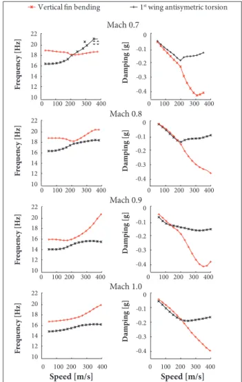
Examining the non-matched point flutter solutions, it is possible to observe that there is an interaction between aeroelastic modes 5 and 7, which are the 1st fin bending and the 1st antisymmetric torsion, including a coupling
Figure 5. Non-matched aeroelastic analysis results — high subsonic range.
0 5 10 15 20 25 30 0 5 10 15 20 25 30
0 100 200 300 400 500 0 100 200 300 400 500 0 100 200 300 400 500 0 100 200 300 400 500
F re q u en cy [ H z] F re q u en cy [ H z]
- 0 . 4 - 0 . 3 - 0 . 2 - 0 . 1
0 D am p in g [ g ] D am p in g [ g ]
- 0 . 6 - 0 . 5 - 0 . 4 - 0 . 3 - 0 . 2 - 0 . 1
0
S p e e d [ m / s ] M a c h 0 .8 0
S p e e d [ m / s ] M a c h 0 .7 0
S p e e d [ m / s ] M a c h 0 .8 0 S p e e d [ m / s ]
M a c h 0 .7 0 W H Z , M o d e 1 W H Z , M o d e 2 W H Z , M o d e 3 W H Z , M o d e 4
W H Z , M o d e 5 W H Z , M o d e 6 W H Z , M o d e 7 W H Z , M o d e 8
W H Z , M o d e 9 W H Z , M o d e 1 0
G , M o d e 1 G , M o d e 2 G , M o d e 3
G , M o d e 4 G , M o d e 5 G , M o d e 6
G , M o d e 7 G , M o d e 8 G , M o d e 9
0 5 10 15 20 25 30 -0.4 -0.3 -0.2 -0.1 0 D am p ing [ g] -0.4 -0.3 -0.2 -0.1 0 D am p ing [ g]
0 100 200 300 400 500
Speed [m/s] - Mach 0.90
0 100 200 300 400 500
Speed [m/s] - Mach 1.0
0 200 500
Speed [m/s] - Mach 0.90
0 100 200 300 400 500
100 300 400
Speed [m/s] - Mach 1.0 0 5 10 15 20 25 30 F re qu en cy [ H z] F re qu en cy [ H z]
WHZ, Mode 1
WHZ, Mode 2
WHZ, Mode 3
WHZ, Mode 4
WHZ, Mode 5
WHZ, Mode 6
WHZ, Mode 7
WHZ, Mode 8
WHZ, Mode 9 WHZ, Mode 10
G, Mode 1
G, Mode 2
G, Mode 3
G, Mode 4 G, Mode 5 G, Mode 6
G, Mode 7
G, Mode 8 G, Mode 9 WHZ: Aeroelastic frequency (Hz); G: Aeroelastic damping (growth rate, non-dimensional).
trend. This coupling mechanism is not critical, mainly obser ved at subsonic conditions (Mach 0.70) and is attenuated with the increase in Mach number. The reason for this behavior lies in the fact that the compressibility effect increases the main lifting surfaces (wings) lift efficiency resulted from a wing torsion motion (mode 5). The increase in the wing unsteady aerodynamic loading implies the increase in aerodynamic stiffness, leading to changes in the aeroelastic natural frequency. Moreover, the increase in lift due to the vertical fin motion does not happen at the same rate because the vertical fin is a smaller lifting surface, when compared to the wings. Because of this, the contribution for the aeroelastic stiffness in the context of the coupling mechanism, even with increased loading characteristics due compressibility effects, should be minimized. The mode shapes involved in this aeroelastic mechanism are presented in Fig. 7.
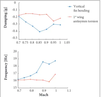
Figure 8 details the aeroelastic coupling mechanism evolu-tion from the non-matched lutter analysis, when the airspeed number increases. For the same aeroelastic mechanism, the
aeroelastic modal evolution is detailed in Fig. 9 for the case of the matched point solution, where the damping and frequency are plotted as a function of light Mach number.
he objective of the aeroelastic analysis is not only identifying possible aeroelastic instabilities, but also observing modal
Figure 7. Mode shapes involved in coupling mechanism.
(a) 5th mode vertical in bending — 15.10 Hz; (b) 7th mode
antisymmetric wing torsion — 16.70 Hz.
0 5 10 15 20 25 30
0.7 0.8 0.9 1
0.7 0.8 0.9 1
Mach
Frequency [Hz]
WHZ, Mode 1 WHZ, Mode2 WHZ, Mode 3 WHZ, Mode 4 WHZ, Mode 5 WHZ, Mode 6 WHZ, Mode 7 WHZ, Mode 8 WHZ, Mode 9 WHZ, Mode 10 -0.4 -0.3 -0.2 -0.1 0 Damping [g]
G, Mode 1 G, Mode 2 G, Mode 3 G, Mode 4 G, Mode 5 G, Mode 6 G, Mode 7 G, Mode 8 G, Mode 9
Mach 0.7
Mach 0.8
Mach 0.9
Mach 1.0
0 100 200 300 400 0 100 200 300 400
0 100 200 300 400 0 100 200 300 400
0 100 200 300 400 0 100 200 300 400
0 100 200 300 400 0 100 200 300 400
Speed [m/s] Speed [m/s]
F re q u enc y [H z] F re q u enc y [H z] F re q u enc y [H z] F re q u enc y [H z] D am p in g [g] D am p in g [g] D am p in g [g] D am p in g [g] -0.4 -0.3 -0.2 -0.1 0 -0.4 -0.3 -0.2 -0.1 0 -0.4 -0.3 -0.2 -0.1 0 -0.4 -0.3 -0.2 -0.1 0 10 12 14 16 18 20 22 10 12 14 16 18 20 22 10 12 14 16 18 20 22 10 12 14 16 18 20 22 -0,45 -0,4 -0,35 -0,3 -0,25 -0,2 -0,15 -0,1 -0,05 0
Vertical fi n bending 1st wing antisymetric torsion
Figure 6. Matched point lutter solution.
Figure 8. Coupling mechanisms for the aircraft, reference Mach number.
173
Comparison of In-Flight Measured and Computed Aeroelastic Damping: Modal Identiication Procedures and Modeling Approaches
parameter evolutions and how they behave. Looking at modes 5 and 7, it is possible to conclude that there is an indication of diiculties on identifying the vertical in bending. Also, at almost the same frequency, there is the antisymmetric wing torsion.
In order to circumvent these difficulties associated to the capability of very close modal parameter or mode shape identiication, the selected mode shapes for correlating with experiments shall be selected as the classical set of modes that might interact to compose a coupled bending-torsion lutter mechanism. he reader should remember that the scope of the present investigations does not predict lutter, but in fact the aeroelastic damping behavior as a function of airspeed.
he selected mode shapes for investigation will be typical mode shapes in terms of easiness for extracting energy from the aerodynamics. Four mode shapes, two symmetric and two antisymmetric, were chosen represented by the 1st wing bending, 1st wing torsion, for symmetric and antisymmetric motions (Fig. 10).
he choice of these mode shapes is justiied by the fact that most of the lutter mechanism involves these kinds of mode shapes, for instance, the bending torsion out of phase coupling. Since lutter prediction is not the goal of the present efort, it is assumed this mode shape set to be correlated with experiments. Furthermore, aeroelastic modal parameter identiication including the four proposed mode shapes is the best option for modal parameters identiication from reduced modal data, in special damping. It is important to note that a symmetric wing
1st symmetric wing bending 1st antisymmetric wing bending
1st symmetric wing torsion 1st antisymmetric wing torsion
Figure 10. Aircraft selected mode shapes for correlation with experiments.
bending and an antisymmetric wing bending are relatively easy to observe even from a small set of measurement points, as well as the symmetric and antisymmetric wing torsions. Figure 10 presents the selected mode shapes for the correlation studies.
OPERATIONAL MODAL ANALYSIS RESULTS
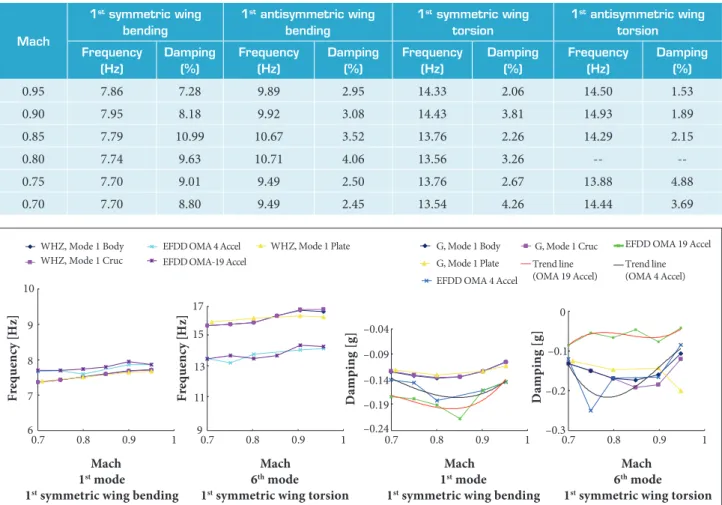
he data were analyzed using the B&K OMA® sotware to identify modal parameters through EFDD/OMA technique. he identiied modes of vibration including frequency and damping factors ξ are shown in Table 2.
Only the selected irst four modes could be well identiied. A possible difficulty might be encountered in the sense of identiication of modal parameters associated to modes 5 and 7, related to the proximity in terms of frequency and mode shape displacement pattern, as one can note from Fig. 6. For this reason the selected mode shape set presented in Fig. 10 was used to compute the corresponding damping and frequency based on the EFDD/OMA technique.
Figure 11 presents a comparison among diferent modeling approaches and two operational modal analysis applications. The numerical approaches used were based in a flat plate, cruciform and panel/body aerodynamic models, as shown in Fig. 1. For the operational modal analyses, the irst case includes 16 measurement points and used the EFDD method; the second one includes four measurement points and used an in-house implementation of the FDD method.
The damping trends observed when comparing the numerical and experimental results show that they behave very similarly. he best correlation in terms of trends is observed
15 16 17 18 19 20
0.7 0.8 0.9 1 1.1
Mach
F
re
qu
en
cy
[
H
z]
-0.5 -0.4 -0.3 -0.2 -0.1 0
0.7 0.75 0.8 0.85 0.9 0.95 1 1.05
D
am
p
ing
[
g
] Vertical
fin bending
1st wing
antisymm torsion
in the 1st symmetrical wing bending. Otherwise, they appear to be shited in the direction of an increased damping as far as the number of accelerometers employed in the analyses was increased. hese results are in conformity with what was indicated by Kehoe (1995), who observed a smaller damping associated to poor data quality, typically obtained with random atmospheric turbulence, aligned to a reduced number of measurement points, as in the case of four accelerometers.
Looking at the 6th aeroelastic mode plot, also in Fig. 11 it is observed that the lowest values in terms of measured damping occurred in the case when the time response of 16 accelerometers were used in the data reduction. Otherwise, when four accelerometers were considered, the measured damping was greater, more scattered, but tending to behave similarly to numerical predictions as a function of the Mach number.
An operational modal analysis was also conducted for the aircrat in the ground, before the light during the taxiing.
he main excitation sources, in this case, are the turbulence in presence of ground effect and the taxiway roughness. he reader should note that this condition difers from the standard free boundary condition. he tyres and landing gear mechanism impose the diferent dynamic boundary conditions instead of the case when the aircrat is suspended in a sot support. he consequence is the increase in terms of structural damping of the irst mode (symmetrical wing bending), when compared to the EMA results for the aircrat suspended in a sot suspension to simulate a free-free boundary condition (Skilling and Burke 1973).
he results presented in Table 3 are useful to understand why the in-light measured damping factors are shited from the corresponding theoretical predictions, as the reader can see in the plot of the irst symmetric wing bending in Fig. 10. One should remember that the theoretically computed aeroelastic damping does not include structural damping in the airframe FEM model.
Mach
1st symmetric wing
bending
1st antisymmetric wing
bending
1st symmetric wing
torsion
1st antisymmetric wing
torsion
Frequency (Hz)
Damping (%)
Frequency (Hz)
Damping (%)
Frequency (Hz)
Damping (%)
Frequency (Hz)
Damping (%)
0.95 7.86 7.28 9.89 2.95 14.33 2.06 14.50 1.53
0.90 7.95 8.18 9.92 3.08 14.43 3.81 14.93 1.89
0.85 7.79 10.99 10.67 3.52 13.76 2.26 14.29 2.15
0.80 7.74 9.63 10.71 4.06 13.56 3.26 --
--0.75 7.70 9.01 9.49 2.50 13.76 2.67 13.88 4.88
0.70 7.70 8.80 9.49 2.45 13.54 4.26 14.44 3.69
Table 2. Identiied modal parameters from EFDD/OMA.
6 7 8 9 10
0.7 0.8 0.9 1
Mach
F
re
qu
e
n
cy
[
H
z]
9 11 13 15 17
0.7 0.8 0.9 1
Mach
F
re
qu
en
cy
[
H
z]
–0.24 –0.19 –0.14 –0.09 –0.04
0.7 0.8 0.9 1
Mach
Damping [g]
WHZ, Mode 1 Body WHZ, Mode 1 C r u c
WHZ, Mode 1 P l a t e E F D D O MA 4 A c c el
EFDD OMA-19 Accel
–0.3 –0.2 –0.1 0
0.7 0.8 0.9 1
Mach
Damping [g]
G, Mode 1 Body G , M o d e 1 C r u c
G , M o d e 1 P l a t e
EFDD OMA 4 Accel
EFDD OMA 19 Accel
Trend line (OMA 4 Accel) Trend line
(OMA 19 Accel)
1st mode
1st symmetric wing bending
1st mode
1st symmetric wing bending
6th mode
1st symmetric wing torsion
6th mode
1st symmetric wing torsion
175
Comparison of In-Flight Measured and Computed Aeroelastic Damping: Modal Identiication Procedures and Modeling Approaches
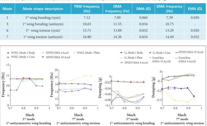
Figure 12. Antisymmetric modes. 8
9 10 11 12
0.7 0.8 0.9 1
Mach
F
re
qu
e
n
cy
[
H
z]
10 14
12 16 18 20
0.7 0.8 0.9 1
Mach
F
re
qu
en
cy
[
H
z]
–0.02
–0.04 –0.06 –0.08 –0.1 0
0.7 0.8 0.9 1
Mach
Damping [g]
WHZ, Mode 1 Body WHZ, Mode 1 Cruc
WHZ, Mode 1 Plate EFDD OMA 4 Accel
EFDD OMA-19 Accel
–0.3 –0.2 –0.1
0
0.7 0.8 0.9 1
Mach
Damping [g]
G, Mode 1 Body G, Mode 1 Cruc G, Mode 1 Plate
EFDD OMA 4 Accel
EFDD OMA 19 Accel
Trend line (OMA 4 Accel) Trend line
(OMA 19 Accel)
3rd m o d e
1 st antisymmetric wing bending
3rd mode
1st antisymmetric wing bending
7th mode
1st antisymmetric wing torsion
7th mode
1st antisymmetric wing torsion
Mode Mode shape description FEM frequency
(Hz)
OMA
frequency (Hz) OMA (G)
EMA frequency
(Hz) EMA (G)
1 1st wing bending (sym) 7.12 7.09 0.060 7.39 0.030
3 1st wing bending (antisym) 10.65 11.55 0.034 10.75
-6 1st wing torsion (sym) 15.71 13.89 0.032 13.29 0.020
7 1st wing torsion (antisym) 16.80 14.36 0.034 14.49 0.032
Table 3. Comparison between experimental and theoretical frequencies and structural modal damping. he antisymmetric aeroelastic modal data are presented in
Fig. 12. hese results are not as good as for the symmetric modes case. Some diiculties arose for identifying the wing torsion. As the reader can observe, very low aeroelastic damping was computed for the 1st antisymmetric torsion mode. A possible reason for these discrepancies is related to the similarity of mode shape patterns when comparing the 5th and 7th mode shapes.
What probably happens here is a mistake in the correlation process used in accordance with MAC criterion. he similar mode shapes, for aeroelastic reasons, such as a slightly phase shit, can be correlated to each other. In the present case, the correlation between the 5th and 7th modes may generate a MAC index greater than the correlation between modes that should be physically the same, in the frequency band limited by the lines before and ater the identiied peak.
his fact is a good reason for taking care when the intention is the identiication of close mode shapes, for example, almost coalesced aeroelastic modes. The analyst needs to be sure the EFDD/OMA method is not underestimating aeroelastic damping at subcritical conditions due to the degree of linear dependency between the coalescing modes. In the case of
lutter mode identiication, special care need to be taken, even knowing that two coalescing mode shapes are out of phase.
Not only damping discrepancies, but also a frequency shit was identiied in the third mode evolution curve. It is possible to note that probably it was identiied the second mode (symmetrical fuselage bending) instead of the antisymmetric wing bending, for Mach numbers 0.70 and 0.75.
he explanation for this discrepancy regards a problem of the modes identiied by the user. hese modes, even from diferent symmetry behavior, present a similar mode shape and near natural frequencies, as it could be seen in Table 1 and Fig. 3. he discrepancy presented in the frequency curve (Fig. 12) is a good example on the care that must be taken in the selection of modes.
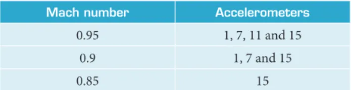
Mach number Accelerometers
0.95 1, 7, 11 and 15
0.9 1, 7 and 15
0.85 15
Table 4. Saturated Accelerometersversus Mach number. the intensity of excitations higher than those provided or the limitation of the sensors themselves in terms of range of limiting acceleration possible to be measured.
here is no evidence if the transonic efects play a role, if unexpected aeroelastic response vibrations caused by shock displacements over the accelerometers can introduce any kind of disturbance. It was also observed an increased number of saturated accelerometers as far as the Mach number increases. Another fact to be highlighted is the position of the accelerometers. Accelerometers 1 and 7 are positioned over the launcher leading edge, accelerometer 15 in the vertical in and accelerometer 11 over the fuselage body. A possible explanation for the saturation of accelerometers 1 and 7 comes from the aeroelastic stifness decrease efect, associated to a dynamic amplification at that position. As far as the airspeed (dynamic pressure) increases, the aeroelastic stifness decreases due to an increase in the aerodynamic stifness, which is proportional to dynamic pressure. hus, the wing structure is more subjected to dynamic ampliications when disturbed around a reference light condition. Table 4 shows the number of sensors which presented saturation.
the aircrat irst four modes of vibration, at reasonable modal parameter values consistent with the theory. Even though some accelerometers signals observed saturation at light conditions within the high subsonic regime, the overall quality of the results is good. A suggested way to circumvent saturation problems is to avoid instrumentation at airframe positions subjected to strong dynamic ampliication efects, such as wing, external store, vertical fin, and tips. Also more robust accelerometers could be selected in terms of load factor range. It is also concluded from the results presented that special care should be taken when using OMA for experimental lutter speeds identiication, either by damping extrapolation or by a lutter margin criterion. his assertion is based on the dispersion of damping measurements, when two coalescing modes are involved. he use of frequency domain decomposition technique (OMA/EFDD) can lead to unrealistic damping predictions, far below the actual values. As a suggestion, for a better modal identiication, it is recommended the use of a suicient number of measurement points for identifying properly the aeroelastic mode shapes. his indication comes from the observation that it was diicult to separate similar mode shapes, when the modal assurance criterion was employed as an indication tool for physically characterization of a given mode of interest.
Furthermore, for the identiication of modes which do not participate in any coupling mechanisms at a particular light condition, this technique could be interesting for a model correlation/validation for updating aeroelastic theoretical models.
he cases studied were limited to the subsonic regime, because in a irst moment the concern is the correlation between theoretical models and light conditions, where it might be expected a linearly-behaved aeroelastic system.
However, it should also be encouraged the use of this technique in the validation of methods for calculating approximate aeroelastic stability solutions under transonic conditions. At least one indication on how the damping evolves, even qualitatively, observing trends as function of Mach number and including a search for possible transonic lutter dip trend, for example. hese results may be important to validate the use of approximate methods at this non-linearly-behaved low conditions.
CONCLUSIONS AND REMARKS
he present investigation indicates, based on theoretical and experimental results correlation, that the proposed OMA, assuming continuous turbulence as input excitation, is a promising methodology for aeroelastic modal parameter identiication. he hypothesis assumed regarding the continuous turbulence being considered as a white noise input led to reasonable results within a low frequency range assumed, for instance, of interest in this study.
177
Comparison of In-Flight Measured and Computed Aeroelastic Damping: Modal Identiication Procedures and Modeling Approaches
Avitabile P (2001) Experimental modal analysis: a simple non-mathematical presentation. Sound and Vibration; [accessed 2016 Apr 15]. http://www.sandv.com/downloads/0101avit.pdf
Batel M (2002) Operational modal analysis — another way of doing modal testing. Sound and Vibration; [accessed 2016 Apr 15]. http:// www.sandv.com/downloads/0208batl.pdf
Bendat JS, Pierson AG (1980) Engineering application of correlation and spectral analysis. New York: John Wiley and Sons.
Borges AS (2006) Análise modal baseada apenas na resposta — decomposição no domínio da freqüência (Master’s thesis). Ilha Solteira: Universidade Estadual Paulista “Júlio de Mesquita Filho”.
Brincker B, Ventura C, Andersen P (2001) Damping estimation by frequency domain decomposition. Proceedings of the IMAC XIX; Kissimmee, USA.
Cauberghe B (2004) Applied frequency-domain system identification in the ield of experimental and operational modal analysis (PhD thesis). Etterbeek: Vrije Universiteit Brussel.
Cooper JE, Emmett PR, Wright JR, Schoeld MJ (1993) Envelope function — a tool for analyzing lutter data. J Aircraft 30(5):785-790.
Dimitriadis G, Cooper JE (2001) Flutter prediction from flight flutter test data. J Aircraft 38(2):355-367. doi: 10.2514/2.2770
Eichenbaum FD (1972) Response of aircraft to three dimensional random turbulence. Technical Report. Marietta: Lockheed-Georgia Co.
Ewins DJ (1986) Modal testing: theory and practice. 3rd ed. Letchworth: Research Studies Press Ltd.
Ferreira LJF (2007) Determinação dos parâmetros dinâmicos da aeronave F-5E a partir das respostas obtidas através de ensaios em voo (Undergraduation paper). São José dos Campos: Instituto Tecnológico de Aeronáutica.
Ferreira LJF, Goes LCS, Marto AG, Silva RGA (2008) In-flight output only modal analysis of aircraft structural dynamics. Proceedings of the SAE Noise and Vibration Conference — NVH 2008; Florianópolis, Brazil.
Follador RC (2009) Análise modal operacional aeroelástica aplicada em ensaios em voo a partir de excitação por turbulência contínua (Master’s thesis). São José dos Campos: Instituto Tecnológico de Aeronáutica.
Hoblit FM (1988) Gust loads on aircraft: concepts & applications. Reston: AIAA.
Kehoe MW (1995) A historical overview of flight flutter testing. Technical Report NASA. Technical Memorandum 4720.
Lind R, Brenner M (2000) Flutterometer: an on-line tool to predict robust flutter margins. J Aircraft 37(6):1105-1112. doi: 10.2514/2.2719
Lind R, Brenner M (2002) Flight test evaluation of flutter prediction methods. Proceedings of the 43rd AIAA/ASME/ASCE/AHS/ASC Structures, Structural Dynamics, and Materials Conference; Denver, USA.
Maia NMM, Silva JMM, He J, Lieven NAJ, Lin RM, Skingle GW, To WM, Urgueira APV (1997) Theoretical and experimental modal analysis. Taunton: Research Studies Press.
Peeters B, De Troyer T, Guillaume P, Van der Auweraer H (2006) In-flight modal analysis: a comparison between sweep and turbulence excitation. Proceedings of the ISMA 2006 International Conference on Noise and Vibration Engineering; Leuven, Belgium.
Pines S (1958) An elementary explanation of the flutter mechanism. Proceedings of Dynamics and Aeroelasticity Meeting; New York, USA.
Silva RGA, Bones CA, Alonso ACP (1999) Proposta de ensaio de flutter em voo no regime subsônico da aeronave F-5E. Technical Report RENG ASA-L 07/99. São José dos Campos: Instituto de Aeronáutica e Espaço.
Silva W, Brenner M, Cooper J, Denegri C, Dunn S, Huttsell L, Kaynes I, Lind R, Poirel D, Yurkovich R (2005) Advanced flutter and LCO prediction tools for flight test risk and cost reduction — an international collaborative program for T&E support. Proceedings of the U.S. Air Force T&E Days; Nashville, USA.
Skilling DC, Burke DL (1973) Ground vibration test F-5E R1003 & R1002. NOR 73-21. Northrop Corporation.
Uhl T, Petko M, Peeters B, Van der Auweraer H (2007) Embedded system for real time flight flutter detection. Proceedings of the 6th International Workshop on Structural Health Monitoring; Palo Alto, USA.
Verboven P (2002) Frequency-domain system identification for modal analysis (PhD thesis). Etterbeek: Vrije Universiteit Brussel.
Zimmerman NH, Weissenburguer JT (1964) Prediction of lutter onset speed based on flight testing at subcritical speeds. J Aircraft 1(4):190-202. doi: 10.2514/3.43581
ZONA Technology, editor (2007) ZAERO Theoretical Manual. Version 8.0. Scottsdale: ZONA Tech.