J. Aerosp. Technol. Manag., São José dos Campos, Vol.8, No 4, pp.408-422, Oct.-Dec., 2016
ABSTRACT: This article highlights both theoretical and experimental experiences in the ield of helmet-mounted cueing systems. The current state of these systems is described as optical and hybrid. The adventures of the positioning under local magnetic ield are considered, and the directions for further improvement of magnetic technology are identiied. A new method is proposed for the local magnetic ield creation to increase update rate, to reduce the inluence of the Earth’s magnetic ield, and to reduce energy consumption of helmet-mounted cueing systems in relation to known prototypes. A mathematical model of positioning ield is offered. The accuracy of the ield mathematical description is studied for different shapes of windings. The transients are investigated in the source of positioning ield and in the interior of the cockpit. In addition, a mathematical model of magnetic measurements is proposed, and the main sources of measurement and positioning errors are investigated. The calculation algorithm of the helmet’s coordinates is considered based on the results of magnetic measurements. The results of physical models research are given, and the operation of a sample in the full range of angles is shown. The trial mapping is conducted for the ield created by the source with a ferromagnetic core. Positioning of the helmet’s movement on speciied paths is performed, and the results make it possible to igure out the next generation of helmet-mounted cueing systems with extended angles range, higher angular and linear accuracy, increased update rate (200 Hz), and minimized inluence of Earth’s magnetic ield.
KEYWORDS: Helmet, Cueing systems, Magnetic ield.
The Magnetic Tracker with Improved
Properties for the Helmet-Mounted
Cueing System
Michail Zhelamskij1
INTRODUCTION
he helmet-mounted cueing system (HMCS) is a device used in modern combat aircraft, which allows the pilot to designate the on-board weapon and other equipment at the target in accordance with the direction of sight. Before the HMCS appeared, in close combat, the pilot had to align the aircrat to shoot at a target. Using the head angle as a pointer to direct the weapons, the pilot can point his head at the target to actuate a weapon. his enables making more attacks, without having to maneuver to the optimum iring position. hese systems allow targets to be designated with minimal aircrat maneuvering, minimizing the time spent in the threat environment and allowing greater lethality, survivability, and pilot situational awareness. hese devices were created irst in South Africa (Mirage F1, mid-1970s), then in the Soviet Union (MIG-29, 1985), Israel (Python-4, 1990) and, inally, in the United States (AIX-9X missile, 1990) (Melzer, 1997). If the position of the helmet is used to point the missile, it thus must be calibrated and it securely on the pilot’s head. hat is why HMCS should be considered from a scientiic point of view.
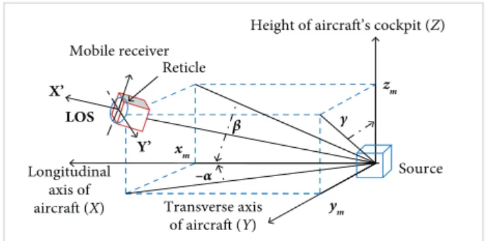
Figure 1 shows the position and orientation of the helmet in the coordinate system of the aircrat. he task of targeting is the orientation calculing of the movable helmet coordinate system X’Y’Z’ in relation to the stationary coordinate system XYZ of aircrat. he line between the pilot’s eye and the reticle on the visor is known as line of sight (LOS) between the aircrat and the intended target. he user’s eye must stay aligned with the sight direction. To do it, the reticle R should be rigidly connected with the helmet and capture the view direction in doi: 10.5028/jatm.v8i4.660
1.Polytechnical University – Department of Measurement and Technologies – Saint Petersburg – Russia.
Author for correspondence: Michail Zhelamskij | Polytechnical University –Department of Measurement and Technologies | Politekhnicheskaya ul., 29 | 195251
Saint Petersburg – Russia | E-mail: [email protected]
J. Aerosp. Technol. Manag., São José dos Campos, Vol.8, No 4, pp.408-422, Oct.-Dec., 2016 409
The Magnetic Tracker with Improved Properties for the Helmet-Mounted Cueing System
relation to it. h erefore, the pilot’s eye always looks at the target through the reticle.
h e new theory is proposed with 6 degrees of freedom (DOF) of magnetic positioning at short distance. The way to organize the local magnetic i eld is described to improve accuracy of cueing. The mathematic models to create and measure the local positioning i eld are suggested. h e proposal determines a concept of the new generation of magnetic trackers with improved properties. h e test results of the i rst magnetic cueing sample are shown.
The results of numerical simulations of coordinates calculations in the positioning i eld are shown, besides the results of the mathematical and physical models investigations. The error estimation of the positioning field descriptions and measurements were done as well as positioning ranges concerning angular and linear displacement.
BASIC DEFINITIONS
It is known the HMCS based on the optical triangulation (Elbit Systems of America® 2016; Buganov 2016; Defencetalk.
com 2007). h e triad of one-by-one light emitting diodes (LEDs) is located on the helmet’s surface. Two i xed on-board receivers are split in the cockpit room. h e coordinates of each LED [xd, yd] on the surface XOY can be obtained from the following system of equations:
Figure 1. Linear position and orientation of mobile receiver relative to the source in the Cartesian coordinate system.
Source Mobile receiver
Height of aircraft’s cockpit (Z)
Reticle
Transverse axis of aircraft (Y) Longitudinal
axis of
aircraft (X) ym
γ
xm
zm
–α β LOS
X’
Y’
HMCS design must sense the elevation, azimuth and roll of the pilot’s head in relation to the aircrat with suffi cient precision even during maneuvering and rapid head movement. h e X’ axis indicates the direction of the target and corresponds to LOS. Azimuth (a) and elevation (b) determine the LOS direction. Linear coordinates x, y, and z of the helmet in the cockpit, calculated by any HMCS, can be used to monitor the pilot’s status. Information about the roll is useful for stabilizing the image on the helmet-mounted display for the accounting of the pilot’s vestibular.
h e range of the helmet linear motion should not be lesser than 1 m. h e precision of cueing, angular error between LOS and derived cue, is determined by the i eld of view (FOV) of the seeker of the air-to-air missile. h e accuracy of the LOS positioning should be much lesser than the FOV of the missile, which is about 1.8° for an infrared heatseeker (Kopp 1982). h e accuracy should be equal over all range of helmet angular motion, and the common field of view of HMCS,angular range over which the sight can still produce a suitably accurate measurement, should be maximum. h e latency or slew rate, how much lag there is between the helmet and the cue, should be minimum. h e weight of helmet-mounted part of HMCS should be minimum, as well as the power consumption. Otherwise, the update frequency should be maximized. It is enough the linear position coordinates accuracy around centimeters. h e roll should be determined with accuracy at the level of units of angular degrees.
Any HMCS includes a movable part, located on the helmet, as well as another item, i xed in the cockpit. Both can be a receiver or a source of local physical i elds. h e computer, also included in HMCS, solves the mathematical positioning task. h e helmet-mounted display will not be considered here.
where: αLand αR are the bearing on each LED from 2 split receivers, obtained from the measurement; KL = −tgαL; KR = −tgαR; AL = x2 × tgαL + y2; AR = x1 × tgαR + y1; the coeffi cients; x1, y1, x2, and y2 are the coordinates of receivers in the cockpit. h e coordinates of the 3 LEDs together with the dimensions of emitting triad are enough to determine the spatial position of the helmet by the methods of analytic geometry, using the solution of Eq. 1 for each LED. h e angular positioning accuracy is at the level of δφ ≥ 45′. h e optical HMCS operates within a cone not greater than ±45°. Accuracy depends on the helmet’s orientation because the helmet itself closes the visibility between LED and receivers, and triangulation triangles are degenerated in the line.
A further approach appeared recently to extend the range of operation of the optical tracker, through the integration of helmet-mounted LEDs together with the gyroscopes and accelerometers (h ales Visionix, Inc. 2016; BAE Systems 2016). Hybrid inertial tracking systems employ a sensitive inertial (1)
1
α
α
α
α
L L d L L d
R R d R R d
( ( )
( ( )
y
К
x
A
y
К
x
A
α β γ Ψ Ψ
α β γ Ψ
)
Δ
ω ΔJ. Aerosp. Technol. Manag., São José dos Campos, Vol.8, No 4, pp.408-422, Oct.-Dec., 2016 410 Zhelamskij M
measurement unit and optical sensor to provide reference to
the aircrat. In the previous operating range, the same optical system is used. Beyond the range of optical tracker, the inertial sensors are used, which have a fundamentally permanent drit of output signals.
Micro-electro mechanical systems (MEMS) contain both gyroscopes and accelerometers and allow to measure full acceleration and orientation of the helmet together with the aircrat movements. It should be taken into account that the full acceleration (a) of the aircrat reaches 10 g during the maneuvers, whereas the head movement, just 0.01 g. An estimation showed that the modern MEMS like ADIS16448 (Analog Devices 2016) measures the helmet’s orientation angles with error at level ∆φ
³
± 0.3 angular degree per second for the aircrat acceleration at the level a = 1 g. In the same condition, the linear coordinates of the helmet are measured with the error at the level ∆x = ± 0.22 × t2 m. It is clear that the angular error exceeds requirements for HMCS during the irst seconds, and the linear coordinates error reaches the level of the percentage meter. hus, hybrid tracker allows expanding the ranges of positioning angles only by short-term use of inertial sensor out of operation range of optical HMCS. Common accuracy in the initial angular range is still determined by the worst element — optical tracker.The magnetic tracking system includes the ixed source
of local magnetic ield, movable receiver on the helmet and
on-board computer, which resolves 3 tasks simultaneously — source controlling, magnetic measurements and coordinates calculation. The procedure of active magnetic positioning intends to establish local non-uniform magnetic ield with a known spatial distribution, in which the magnetic induction measurement is performed using sensors located at the helmet. he calculation of the position and orientation of a movable helmet-mounted receiver is associated with the solving of systems of non-linear equations, which contain the results of independent measurements of magnetic induction at the point of observation under speciied parameters of the ield source (the right parts) and unknown linear and angular coordinates of receiver in space of the positioning ield source (the let parts of equations).
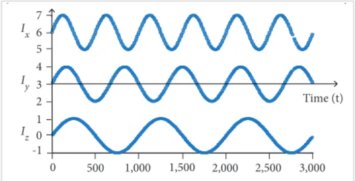
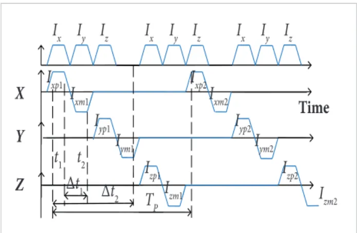
he known active magnetic trackers are based on alternating current (AC) with sinusoidal shape (Fig. 2; Raab 1977) or direct current (DC) with pulse shape (Fig. 3; Blood 1989) local magnetic ield.
he tracker includes 3 orthogonal windings in the ixed source of local magnetic ield and 3 orthogonal sensors in the
mobile receiver. In the irst case (AC), all windings of the source work simultaneously (Ix+ Iy+ Iz) on diferent frequencies. In the second case, they operate in the pulse mode, one by one, in sequence: Ix → Iy→ Iz. he pause (t3–t4) is designed to take into account the Earth’s magnetic ield (EMF), whose inluence is subtracted from each of the measured signals, obtained from the windings.
Time (t) Ix
Iy
Iz
-1 0 1 2 3 4 6 5 7
0 500 1,000 1,500 2,000 2,500 3,000
X
Y
Z
Ix1
t1
M ea s u r ement Pause
Time (t)
t2 t3
t4 Iy1
Iz1
Ix2
Iy2
Iz2
Figure 2. Dimensionless charts of the excitation currents through the windings of the sinusoidal magnetic positioning systems.
Figure 3. Dimensionless charts of the excitation currents in pulse magnetic positioning systems.
In both cases, the coordinates of the helmet are determined from the following equation system solution:
where: Bx, By, and Bz are the computed values of axial components of magnetic ields induction vector, deined by mathematical models of positioning ield, at coordinates of the initial approximation xs, ys, and zs; cos φ, cos ν, and cos ξ are the values of guide cosines of Hall sensor in a ixed coordinate system; Bxxis the measured value of the induction of one sensor from one source winding. Designating Bx × cos φ + By×c os ν + Bz × cos ξ = F and Bxx = Θ, we get:
(2)
(3) 1
α
α
α
α
К
A
К
A
Bxcos + Bycos + Bzcos = Bxx
α β γ Ψ Ψ
α β γ Ψ
)
Δ
ω ΔB
B
Δ Δ1
α
α
α
α
К
A
К
A
F(,X) = - = 0
α β γ Ψ Ψ
α β γ Ψ
)
Δ
ω ΔJ. Aerosp. Technol. Manag., São José dos Campos, Vol.8, No 4, pp.408-422, Oct.-Dec., 2016 411
The Magnetic Tracker with Improved Properties for the Helmet-Mounted Cueing System
w here: ψ = [М, t, Xc, T, C0, IHG, IS, ΔMS, w] is the vector of
parameters included in the mathematical model of establishment and measurement of positioning field, described in Eq. 9. he number of equations M in Eq. 3 shall not be less than the number of the desired coordinates M ≤ N × K, where N is the number of windings in the source and K is the number of sensors in the receiver. he calculation of the 6 coordinates is reduced to the solution of systems (Eq. 3), containing non-linear equations (Eq. 2). In this case, we have: F(X, ψ) = 0, where F is the vector function of X — vector of intended coordinates
at the observation point X = (x, y, z, α, β, γ):
the protective helmet. he main advantage of magnetic methods of positioning is that the LOS is not required between source and receiver. herefore, the helmet cannot inluence the ranges of operation due to transparency for the stationary magnetic ield. his advantage sets out a broad range of the operation angles for magnetic HMCS. As a result, the operation distance — up to 1 m — is comparable with the cockpit size, and the angular range theoretically varies up to ±180°. Positioning accuracy of the magnetic HMCS is better than that of the optical one and declared at the level δX ≤ ±1 mm and δφ ≤ ±0.5 angular degree for up to 1-m distance for the stationary receiver with unchanged orientation.
Dielectric interior elements have no efect on the positioning accuracy for the magnetic method. Electrically conductive materials have efect for AC method only, depending on the size and distance between source, receiver and element. The mapping of the influence of eddy currents on the AC method is labor-intensive (Lescourret 1997) and not always yields the result, particularly for helicopters with cramped cockpits. The practice has shown that AC method cannot be used in helicopters (Egli et al. 1983). Conductive interior elements do not afect the DC method when a certain duration of the magnetic ield pulse is selected (see next). he magnetic materials have efect on both AC and DC magnetic methods, but the magnetic elements in the cockpit interior are much lesser than the electrically conductive materials. herefore, only DC method will be considered further.
he EMF vector is added to the ield positioning. A contribution of EMF depends on the ratio between the object velocity and the update frequency and, for stationary object, it is zero. For DC method, the EMF is taken into account one time per full cycle of the pulse ield switching. he magnetic ield switches to 4 times faster than the output updated, as shown in Fig. 3. his is why the update frequency should be increased more over the current 100 Hz limit to reduce the EMF contribution.
he main parameters of AC and DC trackers, available in the literature, are given in Table 1. he main sources of measurement errors of the positioning ield are shown in Zhelamskij(2014b), among which the inluence of the sensors’ size near the source is dominated as well as their spatial separation and the accuracy of the mathematical description of the positioning ield. he sensors’ size reaches 4 – 5 mm in modern aviation trackers (Kuipers 1975), which leads to increased measurement error of module induction vector near a source up to 10%. herefore, the decreasing in the sensors’ size is actual and accounts for their where: γ is the roll angle.
The desired linear coordinates of mobile receiver [xm, ym, zm], recorded in Eq. 2 as arguments to the mathematical description of the axial component of induction vector,
Bm = [Bx(xm, ym, zm), By(xm, ym, zm), Bz(xm, ym, zm)]T, and
orientation angles of the receiver, [αm, βm, γm], are present in guide cosines through the matrix of the movable receiver rotation: Axyz≡ Ax(α)×Ay(β)×Az(γ). hus, the system (Eq. 4), composed of 6 equations, has a strictly non-linear nature and can only be solved by numerical methods of iterative approximation.
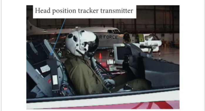
Figure 4 shows a typical layout of magnetic HMCS in the cockpit through the example of the project Vista for the F-16D aircrat (Merryman 1994). A similar layout has another magnetic HMCS (Elbit Systems 2006; Kopp 1998; hales Group 2016). Still in Fig. 4, there is a cubic source of the local magnetic positioning ield, established behind the pilot’s right shoulder. he movable receiver is hidden behind the external surfaces of
Figure 4. Magnetic positioning system of Vista layout aboard the F-16D.
H ead position tracker transmitter
(4) 1
α
α
α
α
К
A
К
A
α β γ Ψ Ψ
α β γ Ψ
1
6
( x, y,z, , , , )
F( X , ) ... 0 ( x, y,z, , , , )
F
F
)
Δ
ω ΔJ. Aerosp. Technol. Manag., São José dos Campos, Vol.8, No 4, pp.408-422, Oct.-Dec., 2016 412 Zhelamskij M
spatial separation, as described next. he already mentioned
aircrat trackers prototypes use either inductive sensors in AC method or luxgate sensor in DC one. In both cases, there are induction measuring windings with large area, which is sensitive to high-frequency interference. herefore, when the sensitivity of measurements is at the level of 10 nTesla, the sustainability of mobile receiver to external disturbances, for example, radar’s radiation, is relevant. А power consumption should be minimized for an on-board equipment in any case. he task is to ind an opportunity to do it. Now we have about 100 W per sphere with 1-m radius. here is important to reduce the value of power consumption for on-board cueing system.
inluence, power consumption, and outer noise immunity. he new mathematical models to create and measure the positioning magnetic ield are presented. he advantages of the new method achieved in comparison with the prototype are described, the estimations of the eddy currents influence are given, and the algorithm of iterative calculation of coordinates of the mobile receiver is considered.
METHODOLOGY
An investigation of new magnetic cueing system was fulilled with the methods described next, such as mathematic description and simulation, system analysis, comparison with known theories, physical modeling of non-standard elements of the system, and the actual movement of the mobile receiver at the inal stage of positioning modeling.
To satisfy the formulated requirements, a new method is proposed to organize the positioning local magnetic ield, and investigations are performed. he new method is theoretically considered as a means of reducing the impact of EMF and power consumption. A mathematical model of the positioning ield is proposed. he investigation of the transition process is performed, as well as of the accuracy of the ield descriptions in the presence of conductive elements. he mathematical model of movable receiver is also proposed and investigated regarding both measurement errors and eliminating the interference from on-board network and external sources. hey are explored in diferent approaches for the iterative solving of the non-linear equations systems, linking the results of magnetic measurements with the desired coordinates. An investigation of the physical models allowed to estimate the mathematical description accuracy of the source with and without ferromagnetic core. Besides, the metrological research of movable receiver was performed. he 6-DOF tracking was fulilled when the receiver was moving at the speciied path.
A new (the 3rd in the world) method to organize the local magnetic positioning ield is called alternating-direct current (ADC) method (Zhelamskij 2011). he bipolar current pulses are ofered in the new method, running consecutively one by one without pause. Figure 5 shows the comparative chart of pulse currents in the source windings for DC prototype, separated by a pause, and for the new ADC method. he top graph is combined for 3 windings of DC method. hree lower graphics are separated for each of the windings of ADC method. In both Title
Source-receiver maximum distance (m)
Update frequency
(Hz)
Static accuracy at the distance of 0.78 m
Polhemus
“Patriot” 1.5 60 ±1.5 mm; ±0.4°
Ascension
“DriveBAY” 0.78 > 120 ±1.4 mm; ±0.5°
Table 1. Comparison of parameters of the prototypes (Polhemus 2016; Ascension Technology Corporation 2016).
J. Aerosp. Technol. Manag., São José dos Campos, Vol.8, No 4, pp.408-422, Oct.-Dec., 2016 413
The Magnetic Tracker with Improved Properties for the Helmet-Mounted Cueing System
cases, the graphics are post-poned for 3 orthogonal windings
of local positioning systems (Raab 1977; Blood 1989), where the magnetic i eld pulses duration is equal. h e graphics are schematically shown. Actually, the rise and fall of pulse current is much lesser than the pulse duration. At the top of each bipolar impulse, the positioning i eld vector is folded with the EMF at a mobile receiver:
Figure 5. Schematic comparison of ADC and DC methods to organize the i eld of positioning.
X
T
ime
I
xt
1t
2∆
t
1∆
t
2
I
xp1I
xp2I
xm1I
xm2I
ym1I
ym2T
PI
yp1I
yp2I
zp1I
zp2I
zm1I
zm2
I
yI
zI
xI
yI
zI
xI
yI
zY
Z
where: B →m is the total induction vector, measured by sensors of the mobile receiver; B →EMF is the EMF vector; B →P is the vector of positioning i eld.
One can write, from Eq. 5, the system of equations for time points t1 and t2, separated by an interval ∆t1, as shown in Fig. 5:
h is system can be resolved relatively to the vector of the positioning i eld B →P. Subtracting the above equations from each other and assuming equality of currents through the source winding |I(+)| = |I(−)| at the moments t1and t2, one can write the common solution of the system (Eq. 6):
The residual value of the EMF, ∆BEMZ = [B →EMF (t1) – B →EMF (t2)],
from Eq. 7, depends on the angular velocity ω of the object and the time interval ∆t1 = t2– t1. h e value ∆BEMZ is zero for the stationary object, when ω = 0.
Hence, taking into account ∆t2 ≥ 2∆t1, the use of bipolar positioning i eld allows to double the amplitude of measured induction versus DC method and reduce twice the impact of EMF:
Besides, the condition ∆t2 ≥ 2∆t1 means twice-increased update rate versus the prototype.
POWER CONSUMPTION FOR ON-BOARD HMCS h e averaged power consumption for DC method (P1) and ADC one (P2) is compared as follows:
where: R is the full resistance of winding; tp is the full period of the windings switching; Ix and Ixpm are the pulse current amplitudes for DC and ADC methods, respectively; T is the duration of one unipolar pulse of positioning i eld, which is equal for both DC and ADC methods.
It can be concluded from Eq. 8:
• If the amplitudes of pulsed current are equal (Ix = Ixp= Ixm), we have (P1/P2)/(3/4) (Fig. 6, mode A).
• If the sweep of measured inductions is equal (BDC = 2BADC), we have (P1/P2)/3 (Fig. 6, mode B).
• If the root mean square (RMS) of noise is given (σN = constant), then the signal-noise ratios for the prototype (SNR1 = B1/ σN) and for the bipolar i elds method (SNR2 = 2 ∙ B2 / σN∙√2 ) are identical (SNR1 = SNR2) for twice-reduced power consumption (P1/P2 = 2), as follows from the calculations (Fig. 6, mode C): (5) (8) (6) (7) 1
α x α К α x α К Ψ
γ
β
α
x
Ψ
γ
β
α
x
Ψ
B BBm EMF P
(
)
)
ω
,
Δ
t
)
Δ
2
Δ
Δ
1 α x α К α x α К Ψ γ β α x Ψ γ β α x Ψ ) ( ) ( ) ( ) ( ) ( ) ( t B t B t B t B t B t B 2 m 2 P 2 EMF 1 m 1 P 1 EMF
)
ω,Δt)Δ
2
Δ Δ
1
α x α К α x α К Ψ
γ
β
α
x
Ψ
γ
β
α
x
Ψ
B (t ) B (t )
B (t) B (t )
B 2
Bmeas m
P 1P 2 EMF 1EMF 2 .
ω
,
Δ
t
)
Δ
2
Δ
Δ
1
α x α К α x α К Ψ
γ
β
α
x
Ψ
γ
β
α
x
Ψ
ω
Δ
Δ
B
Bmeas
2
p, BEMFADCΔ
BEMFDC2
1
Δ
.2 4 2 0 1 6 2 2 0 1 1 p p T x p T xpm p t Rdt t Rdt
I
t
P
P
I
t
σ σ
B
B
Ψ 2Ψ
М
ττ
п пп п п п
2 1 2 2 2
σ σ
N NB
B
, 2 1
2 2
I
I
,2 1 1 2
P
P
.Ψ Ψ
М
ττ п п
п п п п
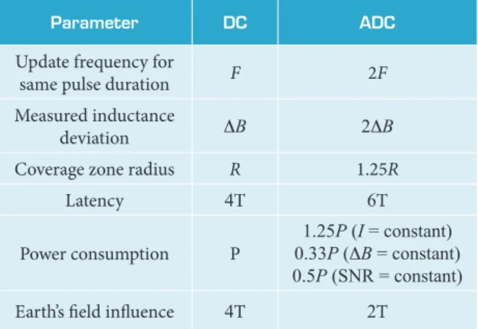
The comparison of the parameters of DC and ADC methods
J. Aerosp. Technol. Manag., São José dos Campos, Vol.8, No 4, pp.408-422, Oct.-Dec., 2016 414 Zhelamskij M
a n d t h e l o w i n g c u r r e n t . I n a c c o r d a n c e w i t h F i g . 6 , f o r t h e s a m e c u r r e n t s , t h e m o d u l e s v a l u e s u s e d t o c a l c u l a t e t h e c o o r d i n a t e s f o r t h e p r o t o t y p e ( B1) and for the new method (B2), which dif er by half, will be read as B1= Ψ/R3 1 and B2= 2Ψ/R3 2. Equating B1 = B2, we get (R2/R1)3 = 2 or R2 = 1.25 × R1.
xm, ym, and zm by one of the positioning i eld source windings on the normal to the sensor surface in the mobile receiver with orientation angles like α, β, and γ (Fig. 1):
Parameter DC ADC
Update frequency for
same pulse duration F 2F
Measured inductance
deviation ΔB 2ΔB
Coverage zone radius R 1.25R
Latency 4Т 6Т
Power consumption P
1.25P (I = constant) 0.33P (ΔB = constant) 0.5P (SNR = constant)
Earth’s i eld inl uence 4Т 2Т Figure 6. Three modes of ADC method operation.
Iy Iz
I= constant
C ur r en t X
A B C
B = constant
SNR = constant
Table 2. Comparison of parameters of the prototype and the new method.
Table 2 shows that the new proposed ADC method provides increased positioning zone radius on 25%, doubles the update rate and the magnitude of measured induction, at least half the impact of EMF, and, up to factor 3, reduces the power consumption. A slight increase in latency can be of -set by the application of Kalman i lter, performing “forward extrapolation”.
where: F1(xm, ym, zm) = [Bx(xm, ym, zm, A, B, I), By(xm, ym, zm, A, B, I), Bz(xm, ym, zm, A, B, I)]T is the function that defines the dependency between the induction vector and the linear coordinates; A and B are the side lengths of the rectangular winding; F2(α, β, γ) = S1r × Axyz is the function of the sensor orientation influence on the measured value, being Axyz≡ Ax(α) × Ay(β) × Az(γ) the full rotation matrix on 3 angles in the sequence α → β → γ and Ax(α), Ay(β), and Az(γ) 3 matrices with size 3 × 3, reflecting the coordinate transformation for the sequential object rotation around each axis of the stationary 3-D Euclidean space XYZ; F3(t) is the function that specifies the sequence of the independent fields over time, as illustrated in Fig. 3, respectively, for the winding X → Y → Z:
Due to the presented advantages, it can be verii ed a new way to organize the positioning i eld, because it better meets the conditions for HMCS as update rate, power consumption, and the impact of EMF.
MATHEMATICAL MODEL
To describe the spatial distribution of the positioning i eld, an expression for the induction vector projection can be written and is created at observation point with coordinates
(9) (10) 2
σ σ
Ψ Ψ
Bm(xm, ym, zm,
,
,
, t) =
(X, М) = F1(xm, ym, zm)
ττ
п пп п п п
T
T
2
σ σ
Ψ Ψ
М
3
1 0
1 2
0 2 6
X
t T ( t ) for T t T
T t T
F
,
ττ
п пп п п п
2
σ σ
Ψ Ψ
М
, 3
0 0 2 4 6
1 2 3
1 3 4
Y
t T , T t T
( t ) for T t T
T t T
F
,F
ττ
п пп п п п
T
T
2
σ σ
Ψ Ψ
М
, 3
0 0 4 1 4 5 1 5 6
Z
t T ( t ) for T t T
T t T
F
(
ττ
п пп п п п
where: T is the half period of bipolar pulse T = ∆t1 = t2 – t1 in Fig. 5.
h e components of the induction vector included in factor F1 of Eq. 9 are fully recorded in Zhelamskij (2014a, 2015) for l at rectangular coils, which have a magnetic moment oriented on each axis of the stationary coordinate system XYZ of aircrat from Fig. 1.
J. Aerosp. Technol. Manag., São José dos Campos, Vol.8, No 4, pp.408-422, Oct.-Dec., 2016 415
The Magnetic Tracker with Improved Properties for the Helmet-Mounted Cueing System
tracking accuracy. h e result of the simulation will allow
verifying requirements for the elements of the distributed source.
To estimate the accuracy of the mathematical model, in any
cases, the amendments ∆B = (BC − BM) ∈ [R] were investigated within the positioning zone R, where BC and BM are, respectively, the calculated and measured values of the induction vector components. At stage of numerical simulation for a coreless source as BM, the values from Eq. 9 were used, written for single thin frame with current. In this case, the value of BC described the result of the calculation for ultimate windings cross-section with dif erent shapes. For the source with ferromagnetic core, the calculation was performed also in accordance with Eq. 9, but measured values BM were taken from the mapping results for the helmet movement zone. As a result, the arrays of the
amendments to the calculated values were obtained, which are used to modify Eq. 2:
(T1 – T2) represents the front duration; (T2 – T4) is the plateau duration; (T4 – T5) is the fall pulse duration.
h e source design should provide the duration of front and fall of the pulse magnetic i eld much less than plateau duration [(T1 – T2) » t] << (T2 – T4).
The mathematical model is created to investigate the inl uence of eddy currents on the accuracy of the positioning i eld measurement. Figure 7 shows a single winding W1of the positioning i eld source, oriented along the X axis of the i xed coordinate system XOY; helmet-mounded receiver R at the observation point with coordinates xm, ym, zm; l at conductive element (EL) with radius r; linear coordinates of the center xd, yd, zd; and direction of the normal to the surface of the element as a matrix of guide cosines NM = [cosφ, cosν, cosυ]T = [0, 1, 0] T , which rel ects the properties of the helicopter cockpit covering (∆ = 2 mm, ρ = 2.7 × 10⁻⁸ Ωm).
where: Bx, By, and Bz are the calculated values of axial
components of the induction vector from Eq. 9; ΔBx, ΔBy, and
ΔBz are the amendments from the mapping results; Bm1 is the full measured value of induction; cosφ, cosν, and cosυ are the guide cosines of the normal to the sensor surface from Eq. 2.
EDDY CURRENTS
Time dependence of the pulsed current I0(t) through the source windings from Eq. 10 may be written in detail in a mathematical model (Eq. 9) as follows:
Figure 7. Design scheme of accounting effects of eddy currents on the interior.
Y Y ’ EL R X’ X yd
xd xm
W1
S ource
2A = 2B
D1 2r D
2
Bm2
Bm1
Bm3 ym
Setting the current through the winding Ix and rectangular winding dimensions 2A and 2B, the mathematical models of the positioning i eld are: BXX = FXX(A, B, Ix,x, y, z), BXY= FXY(A, B, Ix, x, y, z), BXZ = FXZ(A, B, Ix, x, y, z).
h e axial components and module of induction vector Bm1, generated by the winding at the movable receiver, as well as on the surface of the conductive element, Bm2, were calculated from Eq. 9 as shown in Fig. 7. h en, one can estimate the amount of additional i eld at the receiver Bm3, induced by eddy current in the interior EL. The model allows to estimate the ratio Bm1/Bm3 depending on the coordinates of the observation point and the center of the EL disc for dif erent r, ∆, ρ, and NM. h e used formula (Khali n 2004) for additional i eld on the receiver generated by eddy currents in single element of cockpit interior is:
(11) (12) 2 x xpm
σ σ
Ψ
Ψ
М
(
B
x+
B
x)
cos
+ (
B
y+
B
y)
cos
+ (
B
п п
п п
τ п п
T
T
τ
x
x, y, z), B
x, x, y, z), B
x, x, y, z).
2 x xpm
σ σ
Ψ
Ψ
М
cos
+ (
B
z+
B
z)
cos
=
B
m1,
п п
п п
τ п п
τ
x
x, y, z), B
x, x, y, z), B
x, x, y, z).
2
σ σ
Ψ Ψ
М
0 τ 3τ
1
п п N п п п п( t )
( t ) I
F
2
σ σ
Ψ Ψ
М
0 2 1 0 4 2 τ0 4 5
1 1 2 2 1 1 2 2 1 1 2 2
τ
1
п п s N п пt / п п
t
, ( N ) t ( N )
, ( N ) t ( N )
, ( N ) t ( N )
T
T
I
if T
T
T
T
I
if T
T
T
T
if
e
I
T
T
,J. Aerosp. Technol. Manag., São José dos Campos, Vol.8, No 4, pp.408-422, Oct.-Dec., 2016 416 Zhelamskij M
Bosh Sensortec 2016). It is possible to evaluate the possibility of creating the helmet-mounted receiver on such magnetometers t h at w o u l d e l i mi n at e t h e p r o b l e m o f h e l me t’s w e i g ht . T h e immunity of such a device against external interference should be considered as well.
hese magnetometers are intended to measure homogeneous E M F o n l y. T h e ma t h e ma t i c a l mo d e l p r o p o s e d t o a p p l y a mag n e tome te r to me a su re t h e i n h omo ge n e ou s p o s it i on i ng ield (Zhelamskij 2014b) is:
Ater subtracting the equations, we have:
w here: КМ = G(f) × MS(T = const ant ± ∆T) × IHG × IS is t he f u nc t i on w h i ch t a ke s i nto a c c ou nt t he s e ns it iv it y of t he sensor MS, an ampliication G(f) of the measuring channel, the excitation currents through the sensors IHG and ield source IS; BMT = F1(xm, ym, zm) × F2(α, β, γ) × F3(t) is the projection of the induction vector of positioning ield from Eq. 14b to be measured; ∑ 8
k=1εsk (X, Y, Z) is the total systematic measurement error, being εs1the efect of spatial diversity of the receiver’s sensors, εs2 the e f f e c t of t e mp e r atu re , εs 3 t h e mutu a l n on - or t h o g on a l it y of the sensors, εs4 the efect of sensors’ excitation current, εs5 the efect of source excitation current, εs6 the sensitivity uncertainty, εs7 t he er ror of AD C, εs8 t he inluence of s ens ors’ inite size; ∆BEMF(t) is the residual impact of the EMF; ∆BF(x, y, z) is the acc urac y of t he mat hemat ica l des cr iption of t he p osit ioning ield; Ushit(t, T = constant ± ∆T) is the of-set of sensor output voltage; URAND(t) is a random process, modeling its own noise of measurement device.
It c a n b e s e e n f r o m E q . 15 t h a t t h e t o t a l i n d u c t i o n i s BS = BMT(x, y, z, α, β, γ, t) + ∆BEMF(t) + ∆BF(x, y, z), applied to (13)
(14a)
(15)
(14b)
3
К
)
(
)
(
)
(
)
(
)
(
)
(
t
B
t
B
t
B
t
B
t
B
t
B
2 m 2 P 2 400 1 m 1 P 1 400
x,y,z,
(x,y,z)]
ε
x
(x,y,z,
(x,y,z),
Δ
xx
x
xk
Δ
= (x, y, z,
–
3
К
B
(
t
)
B
(
t
)
B
t
B
(
t
B
(
B
meas m(
1)
m(
2))
P 1 P 2
x,y,z, (x,y,z)] ε
x
(x,y,z, (x,y,z),
Δ
x x
x
xk
Δ
= (x, y, z,
–
3
К
(
t
2)
B
400(
t
1)
B
400(
t
2)
2
B
m
x,y,z, (x,y,z)] ε
x
(x,y,z, (x,y,z),
Δ
x x
x
xk
Δ
= (x, y, z,
–
3
К
U
out(t) = {K
M
[B
MT(x,y,z,
,
,
,t) +
B
EMT(t) +
ε
Δ
Δ
–
3
К
(t) +
B
F(x,y,z)]
(1+
8
1
ε
sk k
( x, y,z )
)}+ U
Δ
Δ
–
3
К
ε
z )
)}+ U
shift(t, T) +
Δ
Δ
–
3
К
ε
+U
RAND(t)
Δ
Δ
–
where:
К
1 is the factor to take into account the conductive proper ties of the element EL; S is the projection of the element EL square, visible f rom the windingW
1 (see Fig. 7);D
1 is the distance between EL and the winding;D
2 is distance between EL and the receiver.MAGNETIC INTERFERENCE
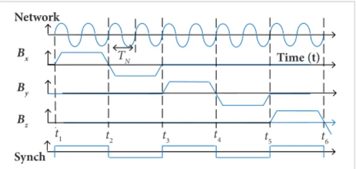
I t i s i mp o r t a n t t o t a k e i n t o a c c o u n t t h e ma g n e t i c i nt e r f e r e n c e f r o m a n o n - b o a r d n e t w o r k o f 400 H z , w h i c h c a n r e a c h 10 – 15% o f t h e a mp l i t u d e o f t h e p o s i t i o n i n g ield. To implement a diferencing metho d of comp ensation, it is ne c e ss ar y t hat t he du r at i on of ha l f of t he bip ol ar pu ls e positioning ield (t2 – t1) be a multiple of the total duration of the periods n ∙ TN of the interference from the on-board network: n ∙ TN = (t2 – t1) = (t3 – t2) = (t4 – t3) = … , as shown in Fig. 8 for n = 2. In this case, t2 − t1 = 5 ms and f = 100 Hz. Correspondingly, for n = 1, t2− t1 = 2.5 ms and f = 200 Hz; for n = 3, t2− t1 = 10 ms and f = 50 Hz. C onsidering BEMF constant and rewriting Eq.
2 in view of the contribution of interference from on-board network in case t2 − t1 = 2n/2f400, it is possible to obtain:
It follows from Eq. 14b that the difference result does not contain the inluence of magnetic interference from the on-board network. The on-board power supply frequency f = 400 Hz is not as stable as in terrestrial networks of 50/60 Hz and depends on the aircrat speed engine. herefore, the duration of the magnetic ield pulse loats and strictly corresponds to the selected number of on-board network half period, using the hardware synchronization as shown in the lower graph of Fig. 8.
ACCURACY
New modern magnetometers with Hall sensors appeared recently, with the minimum weight of the units gram and the size of a millimeter level (Asahi Kasei Corp. 2016; Ivensense® 2016;
Figure 8. Compensation of magnetic interference inluence from the on-board network.
Network
Bx T
N
t1 t2 t3 t4 t5 t6
By
Bz
Synch
T ime (t)
Be
~
K
1∙
S
/(
D
13∙
D
2J. Aerosp. Technol. Manag., São José dos Campos, Vol.8, No 4, pp.408-422, Oct.-Dec., 2016 417
The Magnetic Tracker with Improved Properties for the Helmet-Mounted Cueing System
the sensor, being converted to the measured voltage through
KM with an accuracy of ∑ 8
k=1εsk (X, Y, Z), thus being added the
voltages Us h i t(t, T) and URAND(t), which do not depend on the measured ields induction. As a result, the mathematical model of the systematic positioning error of the ield measurement is proposed:
induction for the assumed coordinates, and Bknm the measured values of induction.
Diferent ways to determine the step in Eq. 18 were applied, like a constant step or the steepest descent method. In addition, it was researched the method of separation of variables into linear and angular, and, for each type of coordinates, it was solved the system of equations.
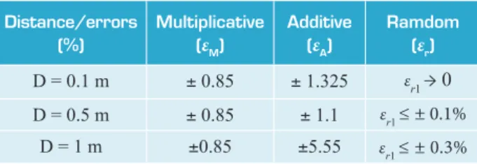
To connect both positioning and measurement errors, Monte Carlo method is applied to investigate the transformation of random measurement errors of positioning field induction (∆BN) into computation errors (∆X) of coordinates. To simulate the noise of ∆BN, centered signals from a random generator were added to induction measurements in each channel: dBx(j) = KN × 2 × (Y(1,1) − 0.5), dBy(j) = KN × 2 × (Y(1,2) − 0.5), and dBz(j) = KN × 2 × (Y(1,3) − 0.5), where: KN = Т × j is the growing scale of the random process amplitude, the same for all channels; Т is the rate of the amplitude growing; Y = rand(1, 3) is the matrix of random uncorrelated numbers, with dimension 1 × 3 in scale 0 – 1. Adding the same random process at all measuring channels models, the impact of external disturbances is dBx(j) = dBy(j) = dBz(j) = KN× 2 × (Y(1,1) − 0.5). It was investigated the dependence of RMS of computed coordinates (σx) versus the RMS of input random process (σBmax). The transformation of multiplicative measurement errors was explored by the Monte Carlo method for coincidence of the real coordinates and initial approximation. In this case, the measured signals were multiplied by KM = 1 + 0.01 × j × εS, being εS the limit value of the multiplicative measurement errors, and j the point number at the interval 0 – 100 with step 1: Bx(j) = Bx(0) × KM; By(j) = By(0) × KM; Bz(j) = Bz
(
0) × KM.he dependence was investigated on residual coordinate deviations
where: P1(D) = εs1(D) + εs7(D) + εs8(D) + εEMF(D); P2 = εs3+ εs2+ εs4+ εs5 + εs6 ≠ f(D); D is the distance between the receiver and the transmitter.
he speciicity of the positioning ield measurements comes from Eq. 16; the error depends not only on the magnitude, but also on the distance D. his fact allows us to consider Eq. 16 as a function of the distance P(D), which has an extremum. he minimization of P(D) was performed by the dichotomy method under the condition:
where: X = (x, y, z, α, β, γ) is the vector of desired coordinates of movable receiver as already mentioned; i is the number of iterations; STEP is the step of the iterative procedure; CF (X ∈ R) = ∑ N
n=1 ∑ K
k=1 ((knc(X) – Bknm)
2 is the functionality to
minimize, being n the number of windings in the source, k the number of sensors in the receiver, Bknc the calculated values of
versus the increasing values of the multiplicative measurement error δBm = f1(j × εS). For the study of transformation of the additive error component, it was suggested adding to the measured signals the following components: Bx(j) = Bx(0) + 0.01 × i × εA× Bx(0), By(j) = By(0) + 0.01 × i × εA× By(0), and Bz(j) = Bz(0) + 0.01 × i × εA× Bz(0), being εA the limit value of the additive measurement errors from Eq. 6, i the step number in the range of 0 – 100 with step 1, and Bx(0) … Bz(0)the values of the vector component of the induction at the observation point. Here, the dependence of dx from Eq. 19
3
К
ε
P(D) =Δ x
x
( D )
B
B
=8 1
Δ
' k xk k
f
x
+ EMF(D) = P1(D) + P2
–
3
К
x,y,z,
(x,y,z)]
ε
x
(x,y,z,
(x,y,z),
Δ
xx
x
xk
Δ
X
i= X
i-1- STEP
grad(CF)
= (x, y, z,
–
4
external disturbances
–
x =
2
2
21
3
x
x
ry
y
rz
z
r
(1
— –
(x − x + (y − y
(16)
(18) (17)
(19)
δ
x =
It is shown next that the condition (Eq. 17) runs at diferent distances D, depending also on the properties of the measuring system. A presented mathematical model of measurements of positioning ield allowed to improve further the magnetic tracking theory as well as to explore the impact of the properties of receiver and analog-digital converters, the inluence of distance, and the errors of mathematical description of the positioning ield. he investigation of this model made it possible to create metrological ensuring of indoor-navigation theory and to formulate the requirements for mobile receiver.
NUMERICAL SIMULATION
Equation 3 can be solved by numerical methods, using the following iterative formula: