J. D. Silva
[email protected] Tel: (081) 3184-7529 University of Pernambuco – UPE Polytechnic School in Recife Environmental and Energetic Tech. Laboratory
Rua Benfica, 455, Madalena 50750-470 Recife, PE, Brazil
in a Trickle Bed Reactor
A mathematical model is developed for a liquid flow on solid particles in a trickle bed reactor. A mathematical formulation is followed based on the liquid-solid model approach where the liquid phase with the (KCl) tracer is treated as a continuum. The physical modeling is discussed, including the formulation of initial and boundary conditions and the description of the solution methodology. Results of mathematical model are presented and validated. The model is validated through comparison using three experimental cases. The optimized values of the axial dispersion (Dax), liquid-solid mass transfer (kLS), and
partial wetting efficiency (FM) coefficients are obtained simultaneously using the objective
function. The behavior of Dax, kLS, and FM is analyzed by the empirical correlations.
Keywords: liquid-solid model, mathematical modeling, experimental, liquid tracer, TBRs
Introduction1
Gas-liquid-solid reactors with the packed bed of solid particles can be operated in three forms, depending upon the orientation of gas-liquid flows. Gas-liquid flows can be concurrently downflows, cocurrently upflows, and downflow of liquid and countercurrent upflow of gas. The reactor in which gas-liquid flows concurrently downflow is conventionally referred to as a trickle bed reactor (Satterfield et al., 1978). The purpose of this work is associated with trickle bed reactors (TBRs). TBRs are very competitive both technologically and economically because they offer many advantages, such as high conversion, small liquid-solid ratio, small resistance to the diffusion of gaseous reactant to the solid surface, and low pressure drop.
TBRs are widely used in industrial applications. The largest applications of TBRs occur in industrial processes, including hydrotreating, hydrodesulfurization, petroleum refining, petrochemical, hydrogenation, oxidation, hydrodenitrogenation, biochemical, and detoxification of waste water industries (Al-Dahhan et al., 1997; Dudukovic et al., 1999; Liu et al., 2008; Ayude et. al., 2008; Augier et al., 2010; Rodrigo et al., 2009).
Mathematical models of TBRs represent an important tool for minimizing the experimental efforts required for developing this equipment in industrial plants. Mathematical modeling and numerical simulation of TBRS are in continuous development,
contributing in a increasing form for the better understanding of processes and physical phenomena of TBRs. Mathematical models have to be validated with experimental data and these experimental data involve complex measurements of difficult accomplishment.
Mathematical modeling of TBRs may involve the mechanisms of forced convection, axial dispersion, interphase mass transport, intraparticle diffusion, adsorption, and chemical reaction. Normally, these models are constructed relating each phase to the others (Silva et al., 2003; Burghardt et al., 1995; Iliuta et al., 2002; Latifi et al., 1997).
The objective of the work is to estimate and describe the behavior of the axial dispersion (Dax), liquid-solid mass transfer
(kLS), and partial wetting efficiency (FM) coefficients using a set of
experiments carried out in a laboratory scale TBR. By comparison the theoretical model is validated using experimental cases.
Nomenclature
AL(z,t) = concentration of the liquid tracer in the liquid
phase, kg m-3
AS(z,t) = concentration of the liquid tracer in the external
surface of solid, kg m-3
Paper received 5 August 2010. Paper accepted 5 February 2011. Technical Editor: Francisco Cunha
aLS = effective liquid-solid mass transfer area per unit
column volume, m2 m-3
Dax = axial dispersion coefficient for the liquid tracer in
the liquid phase, m2 s-1
DL = liquid molecular diffusivity, m2 s-1
dP = diameter of the catalyst particle, m
dr = diameter of the reactor, m
F = objective function
FM = wetting factor, dimensionless
GaL = Galileo number, GaL =d3pgρ2L µL
hd,L = dynamic liquid holdup, dimensionless
i = complex number −1
kLS = liquid-solid mass transfer coefficient, m s-1
kr = reaction constant, kgmol kg-1 s-1
L = height of the catalyst bed, m NL(ξ) = defined function in Eq. (16)
PE = Peclet number, PE = VSL L / Dax
ReL = Reynolds number, ReL = VSLρL dr / µL
ReG = Reynolds number, ReG = VSGρG dr / µG
ScL = Schmidt number, ScL = µL / ρL DL
t = time, s
VSL = superficial velocity of the liquid phase, m s-1
z = axial distance of the catalytic reactor, m ZL(td) = function defined in Eq. (16)
Greek Symbols
αLS = parameter defined in Eq. (11), dimensionless
βS = parameter defined in Eq. (13), dimensionless
εex = external porosity, dimensionless
εP = bed porosity, dimensionless
Ψi (ξ,td) = dimensionless concentration of the tracer in liquid
and solid, i = L, S
η = catalytic effectiveness factor µL = viscosity of the liquid phase, kg m-1 s-1
ξ = parameter defined in Table 1, dimensionless ρL = density of the liquid phase, kg m-3
Mathematical Model
In this work, the modeling adopted is based on the liquid-solid model, which treats the liquid phase (H2O + KCl tracer) as a
Dynamic Evaluation for Liquid Tracer in a Trickle Bed Reactor
the intraparticle diffusion resistance is neglected; (iv) in any position of the reactor the chemical reaction rate within the solid is equal to the liquid-solid mass transfer rate.
- Mass balance for the liquid:
( )
( )
( ) ( )
( )
( )
[
ALz,t ASz,t]
LS a LS k M F
P 1 2 z
t , z L A 2 L , ax D z
t , z L A SL V t
t , z L A L , d h
−
ε − − ∂ ∂ = ∂ ∂ + ∂ ∂
(1)
- The initial and boundary conditions for Eq. (1) are:
( )
z,0 AL,0 LA = (2)
( )
( )
( )
−
+ = =
+ = ∂ ∂
0 , z L A 0 z t , z L A L , ax D
SL V
0 z z
t , z L A
(3)
( )
0L z z
t , z L
A =
= ∂ ∂
(4)
- Combining the chemical reaction rate with the mass transfer rate:
( )
( )
[
ALz,t ASz,t]
krAS( )
z,t P LSa LS
k − = ηε (5)
Equations (1) to (5) can be analyzed with dimensionless variable terms, see Table (1):
Table 1. Summary of dimensionless variables.
dimensionless liquid concentration
(
)
( )
0 , L A
t , z L A d t ,
L ξ =
ψ
dimensionless solid concentrations
(
)
( )
0 , L A
t , z S A d t ,
Sξ =
ψ
dimensionless time
L , d h L
t SL V d
t =
dimensionless coordinate axial direction L z
= ξ
Writing Eqs. (1) to (5) in dimensionless forms:
(
)
(
)
(
)
(
)
(
)
[
L ,td S ,td]
LS 2
d t , L 2
E P
1 d t , L d
t d t , L
ξ ψ − ξ ψ
α − ξ ∂
ξ ψ ∂ = ξ ∂
ξ ψ ∂ + ∂
ξ ψ ∂
(6)
( )
,0 1Lξ =
ψ (7)
(
)
(
)
−
+ = ξ ξ ψ = + = ξ ξ ∂
ξ ψ ∂
1 0 d t , L E P 0 d t ,
L (8)
(
)
01 d t ,
L =
= ξ ξ ∂
ξ ψ ∂
(9)
(
,td)
S(
,td)
S S(
,td)
Lξ −ψ ξ =β ψ ξ
ψ (10)
Equations (6) through (10) include the following dimensionless parameters:
(
)
SL V
L LS a LS k M F P 1
LS= −ε
α (11)
L , ax D
L SL V E
P = (12)
LS a LS k
P r k
S = ηε
β (13)
Analytical Solution
The solution of transport problems in three-phase systems is very complex and usually numerical approximation methods are used. On the other hand, analytical solutions are used for the simple models. Although the analytical solutions are simple, the boundary conditions proposed for these models need a careful attention. The majority of the analytical solutions belong to infinite and semi-infinite field. The analytical solutions for the finite field have been developed by Feike and Torid (1998) and Dudukovic (1982). In this work, the author adopt the analytical procedure in the finite field region (0 ≤ z ≤ L → 0 ≤ξ≤ 1) where the method of separation of variables is used.
The ψS (ξ, td) was isolated from Eq. (10) and it was introduced
in Eq. (6), reducing it to:
( )
(
)
(
)
(
)
d t , L 2
d t , L 2
E P
1 d t , L
d t
d t ,
L −γψ ξ
ξ ∂
ξ ψ ∂ = ξ ∂
ξ ψ ∂ + ∂
ξ ψ ∂
(14)
where:
1 S
S LS
+ β
β α =
γ (15)
The analytical solution of Eq. (14) was obtained by the separation of variables method using the following relation:
(
,td)
NL( )
ZL( )
tdLξ = ξ ∗
ψ (16)
Then, Eq. (14) was separated in two ordinary differential equations with constant coefficients:
( )
( )
0d t L Z 2 d t d
d t L Z d
= λ
+ (17)
( )
( )
( ) 0L N E P 2 d
L N d 2 d
L N 2
d ξ =
λ −γ + ξ
ξ − ξ
ξ
(18)
( )
d t 2 e 2 1 1 2 E P 4 2 i e 2 C 2 1 1 2 E P 4 2 i e 1 C 2 1 e d t , L λ − ξ ξ − λ−γ− + ξ − λ−γ
= ξ ψ
(19)
Transforming Eq. (19) in its trigonometric form:
ξ − λ −γ + ξ − λ −γ = ξ − λ −γ
2 1 1 2 E P 4 2 1 sin i 2 1 1 2 E P 4 2 1 cos 2 1 1 2 E P 4 2 i e (20) ξ − λ −γ − ξ − λ −γ = ξ − λ −γ − 2 1 1 2 E P 4 2 1 sin i 2 1 1 2 E P 4 2 1 cos 2 1 1 2 E P 4 2 i e (21) then:
( )
[
( )
]
2[
sin( )
]
e 2td 1 e 2 K cos 2 1 e 1 K d t ,L −λ
ξ ξ λ ϕ + ξ ξ λ ϕ = ξ
ψ (22)
where:
( )
121 2 E P 4 2 1 − λ −γ
= λ
ϕ (23)
Applying td→∞ to the above equation and using the boundary
conditions given by Eqs. (8) and (9), the eigenvalue expression was obtained:
( )
1 2 E P 2 2 E P 8 2 1 1 2 E P 4 2 2 E P 2 1 4 g cot + λ −γ − λ −γ − λ −γ λ −γ −
= λ
ϕ (24)
Eq. (24) is a transcendental equation and it can be solved graphically. From this solution, the intermediary values for λn as: λn
= (2 n + ½); (n = 0, 1, 2, 3, ...) were found, so that, the global solution for the concentration distribution in the reactor was obtained by Fourier series.
( )
[
( )
]
[
( )
]
d t 2 n e 0 n n n sin 2 1 e n , 2 K n n cos 2 1 e n , 1 K d t , L λ − ∞ = ξ ξ λ ϕ + ξ ξ λ ϕ = ξ ψ∑
(25) where:( )
[
(
)
]
121 2 2 1 n 2 E P 4 2 1 n n − γ − π + = λ
ϕ (26)
K1,n and K2,n are the integral constants and they are obtained by
orthogonality from the initial condition according to the following procedure: (a) Eq. (25) was multiplied by sinϕn(λn)ξ and their initial
condition was introduced; (b) Eq. (25) was then multiplied by cosϕn(λn)ξ and their initial condition was applied; (c) the resulting
equation of items a and b were integrated from 0 to 1, leading to:
( )
n K2,nT2,n( )
n 1 cos n( )
n n , 1 T n , 1K λ + λ = − ϕ λ (27)
( )
n K2,nT4,n( )
n sin n( )
n n , 3 T n , 1K λ + λ = ϕ λ (28)
where the terms T1,n, T2,n, T3,n and T4,n are given by:
( )
{
( )
[
( )
( )
( )
]
( )
[
]
( )
[
[
( )
]
2}}
n n 6 . 25 8 . 0 n n 2 sin 2 n n 16 1 n n 6 . 0 n n cos n n sin 2 . 3 n n n n , 1 T λ ϕ + λ ϕ + λ ϕ + λ ϕ + λ ϕ λ ϕ λ ϕ = λ (29)( )
( )
( )
[
]
( )
( )
[
( )
]
( )
λ ϕ + λ ϕ λ ϕ − λ ϕ λ ϕ + λ ϕ = λ n n 4 . 0 n n cos n n sin 2 . 13 n n 2 sin 3 . 3 2 n n 16 1 n n n n , 2T (30)
( )
{
( )
( )
[
( )
]
( )
( )
[
]
( )
( )
[
( )
]
3}
n n 4 . 10 n n 2 n n sin 2 n n 16 1 n n cos 2 n n 2 . 13 n n 2 cos n n 3 . 3 n n , 3 T λ ϕ − λ ϕ − λ ϕ λ ϕ + λ ϕ + λ ϕ + λ ϕ λ ϕ = λ (31)
( )
{
( ){
[
( )
]
}
( )
( )
[
]
( )
( )
[
( )
]
3}}
n n 4 . 10 n n sin n n cos 2 n n 16 1 n n 2 . 3 2 n n 16 1 n n 2 sin 6 . 1 n n , 4 T λ ϕ − λ ϕ λ ϕ λ ϕ + λ ϕ + λ ϕ + λ ϕ = λ (32)In Equations (27) and (28), the constants K1,n and K2,n were
obtained as:
( )
{
( )
( )
[
( )
]
}
( )
n T3,n( )
n T1,n( )
n T4,n( )
n n , 2 T n n cos 1 n n , 4 T n n sin n n , 2 T n , 1 K λ λ − λ λ λ ϕ − λ − λ ϕ λ= (33)
( )
{
[
( )
]
( )
( )
}
( )
n T3,n( )
n T1,n( )
nT4,n( )
n n , 2 T n n sin n n , 1 T n n cos 1 n n , 3 T n , 2 K λ λ − λ λ λ ϕ λ − λ ϕ − λ= (34)
Equations (33) and (34) were introduced in Eq. (25) resulting:
( )
( )
( ) ( )
[
( )
( ) ( )
( )
( )
( )
]
[
( )
]
[
( )
( )
( )
( )
]
}}
e n2td n n cos n n , 4 T n n sin n n , 3 T 2 1 exp n n cos 1 n n sin 0n T2,n nT3,n n T1,n nT4,n n n n , 1 T n n cos n n , 2 T 2 1 exp n n sin d t , L λ − ξ ξ λ ϕ λ − ξ λ ϕ λ λ ϕ − + ξ ξ λ ϕ ∞
= λ λ − λ λ
Dynamic Evaluation for Liquid Tracer in a Trickle Bed Reactor
For ξ = 1 it is possible to obtain the response at the outlet of the fixed bed by:
( )
ξ∫
=( ) ( )
= ξ
ξ − ξ δ τ ξ ψ = ψ
1
0
d 1 , L d
t
L (36)
hence,
( )
{
[
( )
( )
( )
( )
( )
( )
( )
( )
]
( )
( )
[
( )
]
( )
( )
[
T3,n n T1,n( )
n sin n( )
n]
}
e n2td n n sin 1 n n cos n n cos n n , 4 T0
n T2,n n T3,n n T1,n nT4,n n n n cos n n sin n n , 3 T n n , 2 T 6 . 1 d
t L
λ − λ ϕ λ − λ
λ ϕ + − λ ϕ λ ϕ λ +
∞
= λ λ − λ λ
λ ϕ λ ϕ λ − λ =
ψ
∑
(37)
Materials and Methods
The experiments were realized in a three-phase trickle bed reactor, which consists of a fixed bed with a height of 0.22 m and an inner diameter of 0.030 m with catalytic particles contacted by a cocurrent gas-liquid downward flow carrying the liquid tracer in the liquid phase. The experiments were performed at conditions where the superficial velocities of the gas and liquid phases were maintained at such a level to guarantee a low interaction regime with VSL in the range of 1.0 x 10⁻⁴ m s-1 to 3.0 x 10⁻³ m s-1 and VSG
in the range of 2.0 x 10⁻² m s-1 to 4.5 x 10⁻¹ m s-1 in pilot plant
trickle bed reactors (Ramachandran and Chaudhari, 1983).
Continuous analysis of the KCl tracer, at a concentration of 0.05M, were made using HPLC/UV-CG 480C at the outlet of the fixed bed. The results were expressed in term of the tracer concentrations versus time.
The methodologies applied to evaluate the axial dispersion, liquid-solid mass transfer effect and partial wetting efficiency for the (N2/H2O-KCl/activated carbon) system were:
- comparison of the experimental results with Eq. (37), developed for the system;
- evaluation of the model parameters Dax, kLS and FM; considered as
initial estimates values obtained from correlations in Table (2); - optimization of the model parameters by comparing between the
experimental and calculated data by Eq. (37).
The initial values of Dax, kLS and FM were determined by the
empirical correlations as to Table (2).
To calculate the concentrations within the mathematical model, for the system N2/H2O - KCl / activated carbon, various parameters
have been necessary. These parameters are presented in Table 3.
Table 2. Correlations for the obtainment of the Dax, kLS and FM, the initial values.
Correlations References
(
)
0.61 L Re 55 . 0 axD = (38) Lange et al. (1999)
( )
( ) ( )
0.2r d
p d 5 . 0 L Sc 2 . 0 G R
73 . 0 L R 2 p d LS a
L D ex L , d h 1 514 . 2 LS k
ε − =
(39) Fukushima and Kusaka, (1977)
(
)
(
)
(
)
0.51 L Ga08 . 0 G Re 22 . 0 L Re 40 . 3 M F
−
− =
(40) Burghardt et al. (1990)
Table 3. Summary of intervals of operating conditions for the particle-fluid (Colombo et al., 1976 and Silva et al., 2003).
Category Properties Numerical Values
Operating conditions Pressure (P), atm 1.01
Temperature (T), K 298.00
Superficial velocity of the liquid phase (VSL) x 103, m s-1 6.01 - 0.79
Superficial velocity of the gas phase (VSG) x 102, m s-1 2.50
Standard acceleration of gravity (g), m s-2 9.81
Packing and bed properties Total bed height (L) x 102, m 0.22
Bed porosity (εp) 0.59
External porosity (εex) 0.39
Effective liquid-solid mass transfer area per unit column volume (aLS) x 10-2, m-1
Diameter of the catalyst particle (dp) x 104, m
Diameter of the reactor (dr) x 10 2
, m Density of the particle (ρp) x 10-3, kg m-3
reaction rate constant (kr) x 10-3, kgmol kg-1 s-1
3.97 3.90 3.00 2.56 6.33
Liquid properties Density of the liquid phase (ρl) x 10-3, kg m-3 1.01
Liquid molecular diffusivity (DL) x 107, m2 s-1 6.89
Viscosity of the liquid phase (µl) x 10-4, kg m-1 s-1 8.96
Surface tension (σl) x 102, kg s-2 7.31
Dynamic liquid holdup (hd,l)x101 4.91
Gas properties Density of the gaseous phase (ρg) x 10 1
, kg m-3 6.63
Experiments were performed at constant superficial velocity of the gas phase VSG = 2.50 x 10⁻² m s-1 and the liquid phase varying in
the range of VSL = (6.01 x 10⁻³ to 7.90 x 10⁻⁴) m s-1.
The axial dispersion coefficient, liquid-solid mass transfer coefficient and partial wetting efficiency were determined simultaneously by comparing between the experimental and theoretical data, obtained at the outlet of the fixed bed, subject to the minimization of the objective function (F), given by:
(
)
∑
[
( )
]
[
( )
]
=
ψ −ψ
=
N
1 k
2 Calc k d t L Exp k d t L M
F , LS k , ax D
F (41)
The numerical procedure to optimize these parameters involved an optimization subroutine (Box, 1965). The optimized values of the three parameters, for different liquid phase flows, are reported below in Table 4.
Table 4. Optimized values of the axial dispersion, liquid-solid mass transfer and wetting factor at VSG = 2.50 x 10⁻² m s-1.
Superficial velocity of the liquid phase
Optimized values Objective function
VSL x 103 m s-1 Dax x 107 m2 s-1 kLS x 106 m s-1 FM F x 103
6.01 9.61 7.06 0.57 1.26
5.67 9.21 6.81 0.54 1.24
5.31 8.32 6.67 0.51 1.16
4.95 7.47 6.32 0.47 1.15
4.59 6.77 5.96 0.46 1.12
4.24 5.59 5.78 0.45 1.10
3.89 5.09 5.43 0.43 1.08
3.54 4.47 5.17 0.42 1.07
3.18 3.79 4.97 0.39 1.05
2.83 3.21 4.49 0.37 1.03
2.48 2.87 4.03 0.33 1.01
2.12 2.37 3.67 0.32 0.95
1.78 2.17 2.79 0.27 0.86
1.41 2.12 2.41 0.24 0.78
1.06 2.08 2.09 0.22 0.62
0.79 2.01 1.87 0.21 0.47
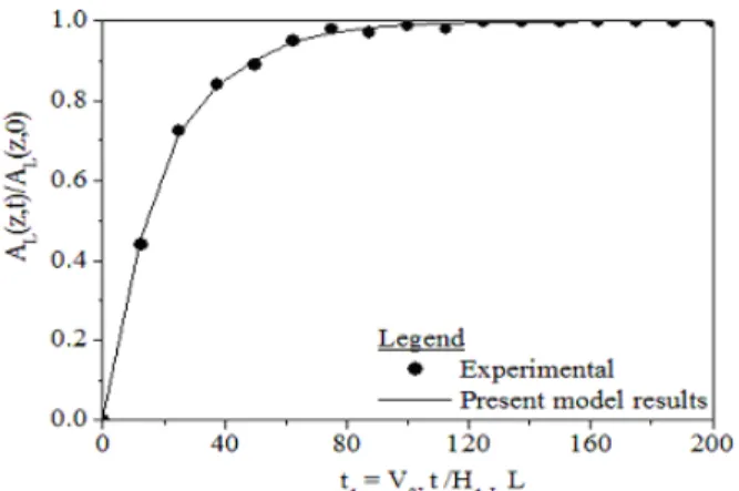
Figure 1. Validation of the tracer concentration at the outlet of the N2/H2O-KCl/activated carbon: ♦♦♦♦ results in gas and liquid superficial velocities VSG = 2.50 x 10⁻²m s-1 and VSL = 2.48 x 10⁻³m s-1; results in parameters Dax = 2.87 x 10⁻⁷ m2s-1, kLS = 4.03 x 10⁻⁶ m s-1, FM = 0.33 and F = 1.01 x 10⁻³.
Figure 2. Validation of the tracer concentration at the outlet of the N2/H2O- KCl / activated carbon: •••• results in gas and liquid superficial velocities VSG = 2.50 x 10⁻²m s-1 and VSL = 2.83 x 10⁻³m s-1; results in parameters Dax = 3.21 x 10⁻⁷ m2s-1, kLS = 4.49 x 10⁻⁶ m s-1, FM = 0.37 and F = 1.03 x 10⁻³.
Figure 3. Validation of the tracer concentration at the outlet of the N2/H2O- KCl / activated carbon: results in gas and liquid superficial velocities VSG = 2.50 x 10⁻²m s-1 and VSL = 5.31 x 10⁻³m s-1; results in parameters Dax = 8.32 x 10⁻⁷ m2s-1, kLS = 6.67 x 10⁻⁶ m s-1, FM = 0.51 and F = 1.16 x 10⁻³.
A model validation process was established by comparing the theoretical results obtained with the values of the optimized parameters and the experimental data for three tests. The results presented in Figs. 1 to 3 confirm this model.
The axial dispersion coefficient, liquid-solid mass transfer coefficient and the wetting efficiency are influenced by changes in the liquid flow. The behavior of Dax, kLS and FM can be described by the
empirical correlations, Eqs. (42), (43) and (44). They are restricted to following operation ranges: dP = 3.90 x10
-4
, 1496 ≤ ReL≤ 178, 0.89 ≤
ScL≤ 4.18 and 0.21 ≤ FM≤ 0.57.
(
)
( )
2.07 M F 18 . 0 L Re 04 . 37 axD = − , R = 0.9982 (42)
(
)
( )
0.23 L Sc 53 . 0 L Re 87 . 2 LSk = , R = 0.9979 (43)
(
)
0.39 L Re 47 . 0 MF = , R = 0.9981 (44)
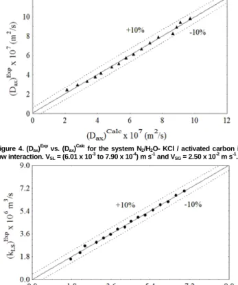
Figures (4), (5) and (6) present parity plots of the obtained results. The parameters Dax, kLS and FM were fitted by the
Dynamic Evaluation for Liquid Tracer in a Trickle Bed Reactor
Figure 4. (Dax)Exp vs. (Dax)Calc for the system N2/H2O- KCl / activated carbon in low interaction. VSL = (6.01 x 10⁻³ to 7.90 x 10⁻⁴) m s-1 and VSG = 2.50 x 10⁻² m s-1.
Figure 5. (kLS)Exp vs. (kLS)Calc for the system N2/H2O- KCl / activated carbon in low interaction. VSL = (6.01 x 10⁻³ to 7.90 x 10⁻⁴) m s-1 and VSG = 2.50 x 10⁻² m s-1.
Figure 6. (FM)Exp vs. (FM)Calc for the system N2/H2O- KCl / activated carbon in low interaction. VSL = (6.01 x 10⁻³ to 7.90 x 10⁻⁴) m s-1 and VSG = 2.50 x 10⁻² m s-1.
Conclusion
Based on the experimental and modelling studies of the liquid phase in a low interaction system, the following results were obtained: (i) the estimation of the parameters Dax, kLS and FM, (ii) the validation
of the model and (iii) the analysis of the behavior of the axial dispersion coefficient, liquid-solid mass transfer coefficient and wetting efficiency by new forms of empirical correlations, Eqs. (42), (43) and (44). The final values of the parameters were obtained with values of the objective function, F = 1.26 x 10⁻³ to 4.70 x 10⁻⁴. Thus, the range of the optimized values of the parameters by fitting between the theoretical and experimental response was given as: Dax = 9.61 x
10-7 m2 s-1 to 2.01 x 10⁻⁷ m2 s-1, kLS = 7.06 x 10⁻⁶ m s-1 to 1.87 x 10⁻⁶ m s-1
and FM = 0.57 to 0.21.
Acknowledgements
The authors would like to thank CNPq (Conselho Nacional de Desenvolvimento Tecnológico) for financial support (process 483541/07-9).
References
Al-Dahhan, M.H., Larachi, F., Dudukovic, M.P., Laurent, A., 1997, “High-pressure trickle bed reactors: a review”, Industrial Engineering
Chemical Research, Vol. 36, pp. 3292-3314.
Augier, F., Koudil, A., Muszynski, L., Yanouri, Q., 2010, “Numerical approach to predict wetting and catalyst efficiencies inside trickle bed reactors”,Chemical Engineering Science, Vol. 65, pp. 255-260.
Ayude, A., Cechini, J., Cassanello, M., Martínez, O., Haure, P., 2008, “Trickle bed reactors: effect of liquid flow modulation on catalytic activity”,
Chemical Engineering Science, Vol. 63, pp. 4969-4973.
Box, P., 1965, “A new method of constrained optimization and a comparison with other method”, Computer Journal, Vol. 8, pp. 42-52.
Burghardt A., Bartelmus G., Jaroszynski M., Kolodziej A., 1995, “Hydrodynamics and mass transfer in a three-phase fixed bed reactor with concurrent gas-liquid downflow”, Chemical Engineering and Processing, Vol. 28, pp. 83-99.
Burghardt A., Kolodziej, A.S., Jaroszynski M., 1990, “Experimental studies of liquid-solid wetting efficiency in trickle-bed concurrent reactors”,
Chemical Engineering Journal, Vol. 28, pp. 35-49.
Colombo A.J., Baldi G., Sicardi S., 1976, “Solid-liquid contacting effectiveness in trickle-bed reactors”, Chemical Engineering Science, Vol. 31, pp. 1101-1108.
Dudukovic, M.P., Larachi, F., Mills, P.L., 1999, “Multiphase reactors-revisited”, Chemical Engineering Science, Vol. 54, pp. 1975-1995.
Dudukovic M.P., 1982, “Analytical solution for the transient response in a diffusion cell of the wickle- kallenbach type”, Chemical Engineering Science, Vol. 37, pp. 153-158.
Feike J. L., Toride N., 1998, “Analytical solutions for solute transport with binary and ternary exchange”, Soil Sci. Soc. Am. J, Vol. 56, pp. 855-864.
Fukushima, S., Kusaka, K., 1977, “Interfacial area boundary of hydrodynamic flow region in packed column with concurrent downward flow”,
Journal of Chemical Engineering of Japan, Vol. 10, No. 6, pp. 461-467. Iliuta, I, Bildea, S.C., Iliuta, M.C., Larachi, F., 2002, “Analysis of trickle-bed and packed bubble column bioreactors for combined carbon oxidation and nitrification”, Brazilian Journal of Chemical Engineering, Vol. 19, pp. 69-87.
Lange, R., Gutsche, R., Hanika, J., 1999, “Forced periodic operation of a trickle-bed reactor”, Chemical Engineering Science, Vol. 54, pp. 2569-2573.
Latifi, M.A., Naderifar, A., Midoux, N., 1997, “Experimental investigation of the liquid-solid mass transfer at the wall of trickle-bed – Influence of Schmidt Number”, Chemical Engineering Science, Vol. 52, pp. 4005-4011.
Liu, G., Zhang, X., Wang, L., Zhang, S., Mi, Z., 2008, “Unsteady-state operation of trickle-bed reactor for dicyclopentadiene hydrogenation”,
Chemical Engineering Science, Vol. 36, pp. 4991-5001.
Ramachandran P.A., Chaudhari, R.B., 1983, “Three phase catalytic reactors”, Gordan and Breach Science Publishers, New York, U.S.A., Chap. 7, pp. 200-255.
Rodrigo J.G., Rosa, L., Quinta-Ferreira, M., 2009, “Turbulence modelling of multiphase flow in high-pressure trickle reactor”, Chemical
Engineering Science, Vol. 64, pp. 1806-1819.
Satterfield, C.N., Van Eck, M.W., Bliss, G.S., 1978, “Liquid - Solid mass transfer in packed beds with downflow cocurrent gas-liquid flow”,
Aiche J., Vol. 24, pp. 709-721.