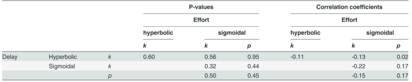
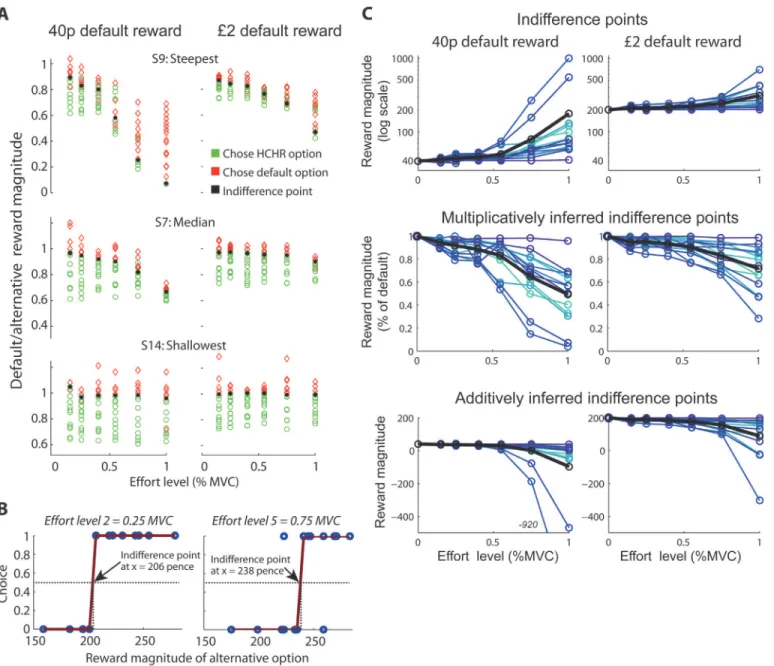
Behavioral modeling of human choices reveals dissociable effects of physical effort and temporal delay on reward devaluation.

However, because of the difficulty of obtain- ing data on morbidity with respect to injuries with lower severity that do not imply death or hospitalization but that have a high

In the second period, 30 days after using herbicide on the trunks of jackfruit trees, it could be observed a shift of individuals from normal into senescent category Table 1...

Mesmo com o texto do repórter fazendo referência à cidade onde ele está e o aspecto de abandono da região, a câmera permanece imóvel, sem fazer um movimento que permiti- ria

Comparison of fecundity and egg size of Leander paulensis with other palaemonids reveals that this species produces a large number of relatively small eggs, with no

Neste sentido pode entender-se que esta visibilidade da experiência técnica torna a peça uma plataforma comunicacional, um denominador comum, logo um elemento

The results show that government spending shocks, in general, have a small effect on GDP; lead to important “crowding-out” effects; have a varied impact on housing prices and

These forecast an expanding SaaS market and that this model will have more significant impact on organizations (both large and small) meaning that research into the determinants

Em primeiro lugar, apesar do valor médio de F2 não diferir de forma significativa entre as faixas etárias em estudo, verifica-se que, no género masculino, o F2 diminui ligeiramente