Uniformity

UNCORRECTED

PROOF

Uniformity

M.F. Brilhante, M. Malva, S. Mendonc¸a, D. Pestana, F. Sequeira,

and S. Velosa

1

Introduction

Let us assume that the p-values fpkgn_kD1 are known from testing H0k vs. HAk, 6

k _{D 1; : : : ; n, in n independent studies on some common issue, and our aim is} 7

to achieve a decision on the overall question H₀! W all the H0k are true vs: HA! W 8

some of the HAk are true. As there are many different ways in which H₀! can be 9

false, selecting an appropriate test is in general unfeasible. On the other hand, 10

combining the available pk’s so that T .p1; : : : ; pn/ is the observed value of a 11

random variable whose sampling distribution under H₀! is known is a simple 12

issue, since under H!

0, p D .p1; : : : ; pn/is the observed value of a random sample 13

P _{D .P}1; : : : Pn/ from a standard uniform population. In fact, several different 14

sensible combined testing procedures are often used [6, 11]. 15

M.F. Brilhante (!) AQ1

Universidade dos Ac¸ores (DM) and CEAUL, Rua da M˜ae de Deus, Apartado 1422, 9501-801 Ponta Delgada, Portugal

e-mail: fbrilhante@uac.pt M. Malva

Escola Superior de Tecnologia de Viseu and CEAUL, Campus Polit´ecnico de Viseu de Repeses, 3504-510 Viseu, Portugal

e-mail: malva@estv.ipv.pt S. Mendonc¸a_{" S. Velosa}

Universidade da Madeira (DME) and CEAUL, Campus Universit´ario da Penteada, 9000-390 Funchal, Portugal

e-mail: smfm@uma.pt; sfilipe@uma.pt D. Pestana_{" F. Sequeira}

Universidade de Lisboa, Faculdade de Ciˆencias (DEIO) and CEAUL, Bloco C6, Piso 4, Campo Grande, 1749-016 Lisboa, Portugal

e-mail: dinis.pestana@fc.ul.pt; fjsequeira@fc.ul.pt

J.L. da Silva et al. (eds.), Advances in Regression, Survival Analysis, Extreme Values,

Markov Processes and Other Statistical Applications, Studies in Theoretical and Applied Statistics, DOI 10.1007/978-3-642-34904-1 7,

© Springer-Verlag Berlin Heidelberg 2013

UNCORRECTED

PROOF

not a sample from a standard uniform population. Recently Paul [10] discussed new

AQ2 17

characterizations of the uniform population, but as they are formulated in terms of 18

expected values, they did not lead directly to new simple tests of uniformity. Gomes 19

et al. [5] exploited the possibility of using computationally augmented samples 20

to test uniformity, with the surprising result that power can decrease with sample 21

augmentation in the class of alternatives they used. Sequeira [12] explains why this 22

is so, and in Sect. 2 below we further discuss the question. In this chapter we use 23

Sukhatme’s transformation to suggest new ways of dealing with the matter. 24

Sukhatme’s [13] transformation, from which R´enyi’s representation of expo- 25

nential order statistics can easily be derived, appears in David and Nagaraja ([2], 26

p. 17–18) and in Johnson et al. ([8], p. 305), with slightly different presentations, 27

applied to the study of exponential and of uniform order statistics, respectively. 28

Durbin [4] used ordered spacings of the uniform to investigate the construction of 29

exact tests. In Sect. 3 we use a Sukhatme’s like transformation to augment the set 30

of order statistics from a uniform parent, and in Sect. 4 we investigate power issues 31

when they are used in testing uniformity. 32

2

Uniformity Versus Mixtures of Uniform and Beta(1,2)

Gomes et al. [5] introduced the family fXmgm2Œ#2;2! of absolutely continuous 34

random variables, with probability density function fXm.x/D

!

mx! m#2₂ "I.0;1/.x/ 35

(the uniform density corresponds to m D 0; for m 2 .0; 2!, Xm is a 36

convex mixture of Beta(1,1) and Beta(2,1), and for m 2 Œ!2; 0!, Xm is 37

a mixture of Beta(1,1) and Beta(1,2)). Observe that for all m 2 Œ!2; 0/, 38

P ŒXm" x! ! P ŒU " x! D m₂ x .x! 1/ > 0 for all x 2 .0; 1/, and thus pseudoran- 39

dom numbers generated by Xmtend to be closer to 0 than pseudorandom numbers 40

generated by a standard uniform random variable U . Thus this family can give 41

important hints on nonuniformity of the set of p-values, cf. the concepts of random 42

p-values in Kulinskaya et al. [9] and of generalized p-values in Hartung et al. [6]. 43

Observe also that for m 2 .0; 2!, Xm tends to take values closer to 1 than the 44

X0_Uniform.0; 1/ random variable, and hence in that range of values it provides 45

a suitable alternative in the case of right one-tailed alternative tests. Moreover, the 46

inverse of the corresponding distribution function is 47

F_X#1 m.u/ D m 2 ! 1 C q!m 2 ! 1 "2 C 2mu m 48

and the generation of pseudo-random numbers from Xm for simulation studies is 49

therefore straightforward. 50

Let U and X be two independent standard uniform random variables. The 51

random variables V D U C X ! IŒU C X!, where IŒx! denotes the largest integer 52

not greater than x, and W D min!U X;

1#U 1#X

"

UNCORRECTED

PROOF

to assess the power of detecting non-uniformity when the sample comes in fact from 55

Xm, m 2 Œ!2; 0!, with the strange result that power does not improve for increased 56

samples. 57

The explanation is however simple: if Xmand Xp are two independent random 58

variables, with m; p 2 Œ!2; 2!, then min#Xm Xp; 1_#Xm 1#Xp $ _d D Xmp 6 [1]. Hence, in case 59

the algorithm uses uniform pseudorandom numbers to augment the sample, the 60

augmented slice will in fact be a uniform subsample, and power decreases. Brilhante 61

et al. [1] present better results using left-skewed parent pseudorandom numbers. 62

Still, the use of the family fXmgm2Œ#2;2! has many advantages, and instead of 63

augmenting the sample externally, as in the above-mentioned papers, by using 64

VmD U C Xm! IŒU C Xm!and WmD min

# U Xm; 1#U 1#Xm $

, with the spurious effect 65

of always generating uniform pseudo p-values, we can use an alternative approach 66

when the purpose is to test the null hypothesis of uniformity vs. Xmparent: 67

• Choose at random one pj 2 fpkgn_kD1. 68

• Generate n ! 1 pseudo p’s of the form min#pj pk ;

1_#pj 1#pk

$

; k_{¤ j .} 69

3

Order Statistics, Spacings and Sukhatme’s Transformation

Let X D .X1; X2; : : : ; Xn/ be a random sample from the absolutely con- 71

tinuous positive random variable X with probability density function fX and 72

.X1Wn; X2Wn; : : : ; XnWn/ the corresponding vector of ascending order statistics. For 73

convenience we assume that left-endpoint ˛X D 0 and we define X0Wn D ˛X D 0. 74

The joint probability density function of the spacings Sk D XkWn! Xk#1Wn, k D 75

1; : : : ; n, is 76

f.S1;S2;:::;Sn/.s1; s2; : : : ; sn/ D nŠ f.X1;X2;:::;Xn/.s1; s1C s2; : : : ; s1C # # # C sn/ 77

(sk > 0, k D 1; : : : ; n, and if the right-endpoint !X is finite,Pn_kD1sk < !X; in 78

this case we can consider the rightmost spacing SnC1 D !X ! XnWn, but this can 79

be expressed as a function !X !PnkD1Sk). Hence, the joint probability density 80

function of the ascending reordering of those n spacings is 81

f.S_1Wn;S_2Wn;:::;S_nWn/.y1; y2; : : : ; yn/D .nŠ/2f.X1;X2;:::;Xn/.y1; y1C y2; : : : ; y1C # # # C yn/ 82

where 0 < y1< : : : < ynandPnk_D1yk < !X. 83

Now define 84

Wk D .n C 1 ! k/.SkWn! Sk#1Wn/; k D 1; : : : ; n; 85

(similar to Sukhatme’s transformation, as defined in David and Nagaraja [2], but 86

UNCORRECTED

PROOF

f.W1;W2;:::;Wn/.w1;w2; : : : ;wn/D nŠ f.X1;X2;:::;Xn/ !w1 n ; 2w1 n C w2 n!1; : : : ;w1C # # # C wn " 89

wk > 0, k D 1; : : : ; n, (observe that the k-th argument is 90

kw1 n C .k! 1/w2 n! 1 C # # # C .k_{C 1 ! j /w}j nC 1 ! j C # # # C wk nC 1 ! k ; k D 1; : : : ; n/; 91 and the joint probability density function of the vector of partial sums Yk D 92

Pk jD1Wj, k D 1; : : : ; n, is 93 f.Y1;Y2;:::;Yn/.y1; y2; : : : ; yn/D nŠ f.X1;X2;:::;Xn/ # y1 n; : : : ; k X jD1 .kC1!j /.yj!yj_!1/ nC1!j ; : : : ; yn $ 94

with 0 < y1 < : : : < ynand the convention y0 D 0. 95

If X _ Uniform.0; !X/, then 96 f.X1;X2;:::;Xn/ # y1 n; : : : ; k X jD1 .kC1!j /.yj!yj!1/ nC1!j ; : : : ; yn $ D _!1n X D f .X1;X2;:::;Xn/.y1; y2; : : : ; yn/; 97 and hence .Y1; Y2; : : : ; Yn/ d D .X1Wn; X2Wn; : : : ; XnWn/.1 98

This suggests that uniformity can be investigated testing whether fXkWngn_kD1 and 99

fYkgn_kD1can be considered samples from the same distribution. Unfortunately, under 100

the null hypothesis that the parent distribution is standard uniform, the two vectors 101

are not independent since we can re-express Yk D Pkj_D1SjWn C .n ! k/SkWn;and 102

consequently Yn D XnWn. Thus, the Smirnov two-sample test is of no use in the 103

present situation. 104

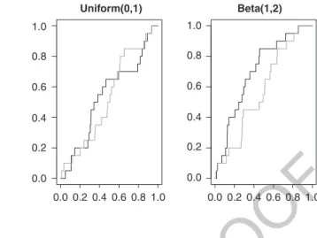
However, the observation of Fig. 1, where we compare the empirical distribution 105

function (edf) corresponding to the order statistics xkWn(black) and the yk (gray), in 106

case of uniform and Beta(1,2) parents, suggests that D!

n D supxjFn!.x/! Gn!.x/j, 107

where F!

n stands for the order statistics edf and Gn!for the accumulated yk edf, will 108

be greater under the alternative HA W X nonuniform with support (0,1) than under 109

the null hypothesis H0 W X _ Uniform.0; 1/. 110

1_{Observe that if !}

X < 1, we can consider n C 1 spacings, with SnC1 D !X # XnWn; of

course in this situation SnC1; SnC1WnC1and WnC1(where in this case it is convenient to use the

transformation

WkD .n C 2 # k/.SkWnC1# Sk!1WnC1/;

as in Johnson et al. [8], p. 305) can be expressed as simple functions of the predecessor members of the sequence. We still get the result that .Y1; Y2; : : : ; Yn/

d

D .X1Wn; X2Wn; : : : ; XnWn/in case of

UNCORRECTED

PROOF

functions F20"and G20" for

Uniform(0,1) and Beta(1,2) parents; this illustrates the general pattern

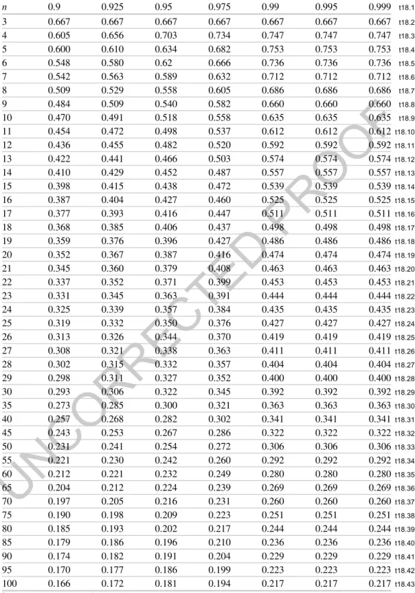
For uniformity testing purposes we present in Table 1 the upper critical points of 111

D_n!, n D 3.1/30.5/100, when the underlying parent is standard uniform .U D Xd 0/. 112

These points were obtained by generating 10,000 independent replicates of the 113

sample .D_n;1! ; D_n;2! ; : : : ; D_n;50! / and defining the quantile of order p of D_n! as the 114

mean of the samples quantiles for p D 0:9, 0.925, 0.95, 0.975, 0.99, 0.995, 0.999. 115

We also performed a simulation study of the proportion of rejections of unifor- 116

mity when the underlying parent was Xm, m 2 Œ!2; 0! and when making pairwise 117

comparisons of the order statistics fxkWng edf and the fykg edf (the process of 118

generating fykg was iteratively repeated 10,000 times). Observe that the rationale 119

for this procedure relies on the fact that if the original observations fpkg are indeed 120

uniform, the “Sukhatme’s” fykg would be order statistics of standard uniform, and 121

hence repeating Sukhatme’s algorithm we would obtain again a set of order statistics 122

of standard uniform. 123

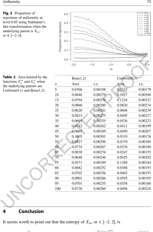
From Fig. 2 we observe that the proportion of rejections of uniformity increases 124

with n. However, the extended Sukhatme’s like transformed data performs badly 125

in detecting departures from uniformity when n < 20. This situation can obviously 126

constitute a problem when combining p-values in meta-analytical syntheses since 127

the number of available (reported) p-values is usually small. 128

Another way of assessing the usefulness of this extended Sukhatme’s transfor- 129

mation in testing uniformity is by calculating the area limited by the edf’s F!

n and 130

G_n!, since under the validity of the null hypothesis X _ Uniform.0; 1/, the area 131

between the two curves should be zero—big area values should indicate a departure 132

from uniformity. In Table 2 we compare the areas obtained by simulation (10,000 133

runs) for some values of n when the underlying parents are standard uniform and 134

Beta(1,2). Analyzing Table 2 we see that the area is indeed inferior for the standard 135

uniform parent, except for some few cases. However, the differences between the 136

two areas can be very small, which can difficult the task of testing uniformity with 137

UNCORRECTED

PROOF

Table 1 Critical points of D"n when the underlying parent is Uniform (0,1)a

t18.1 n 0.9 0.925 0.95 0.975 0.99 0.995 0.999 t18.2 3 0.667 0.667 0.667 0.667 0.667 0.667 0.667 t18.3 4 0.605 0.656 0.703 0.734 0.747 0.747 0.747 t18.4 5 0.600 0.610 0.634 0.682 0.753 0.753 0.753 t18.5 6 0.548 0.580 0.62 0.666 0.736 0.736 0.736 t18.6 7 0.542 0.563 0.589 0.632 0.712 0.712 0.712 t18.7 8 0.509 0.529 0.558 0.605 0.686 0.686 0.686 t18.8 9 0.484 0.509 0.540 0.582 0.660 0.660 0.660 t18.9 10 0.470 0.491 0.518 0.558 0.635 0.635 0.635 t18.10 11 0.454 0.472 0.498 0.537 0.612 0.612 0.612 t18.11 12 0.436 0.455 0.482 0.520 0.592 0.592 0.592 t18.12 13 0.422 0.441 0.466 0.503 0.574 0.574 0.574 t18.13 14 0.410 0.429 0.452 0.487 0.557 0.557 0.557 t18.14 15 0.398 0.415 0.438 0.472 0.539 0.539 0.539 t18.15 16 0.387 0.404 0.427 0.460 0.525 0.525 0.525 t18.16 17 0.377 0.393 0.416 0.447 0.511 0.511 0.511 t18.17 18 0.368 0.385 0.406 0.437 0.498 0.498 0.498 t18.18 19 0.359 0.376 0.396 0.427 0.486 0.486 0.486 t18.19 20 0.352 0.367 0.387 0.416 0.474 0.474 0.474 t18.20 21 0.345 0.360 0.379 0.408 0.463 0.463 0.463 t18.21 22 0.337 0.352 0.371 0.399 0.453 0.453 0.453 t18.22 23 0.331 0.345 0.363 0.391 0.444 0.444 0.444 t18.23 24 0.325 0.339 0.357 0.384 0.435 0.435 0.435 t18.24 25 0.319 0.332 0.350 0.376 0.427 0.427 0.427 t18.25 26 0.313 0.326 0.344 0.370 0.419 0.419 0.419 t18.26 27 0.308 0.321 0.338 0.363 0.411 0.411 0.411 t18.27 28 0.302 0.315 0.332 0.357 0.404 0.404 0.404 t18.28 29 0.298 0.311 0.327 0.352 0.400 0.400 0.400 t18.29 30 0.293 0.306 0.322 0.345 0.392 0.392 0.392 t18.30 35 0.273 0.285 0.300 0.321 0.363 0.363 0.363 t18.31 40 0.257 0.268 0.282 0.302 0.341 0.341 0.341 t18.32 45 0.243 0.253 0.267 0.286 0.322 0.322 0.322 t18.33 50 0.231 0.241 0.254 0.272 0.306 0.306 0.306 t18.34 55 0.221 0.230 0.242 0.260 0.292 0.292 0.292 t18.35 60 0.212 0.221 0.232 0.249 0.280 0.280 0.280 t18.36 65 0.204 0.212 0.224 0.239 0.269 0.269 0.269 t18.37 70 0.197 0.205 0.216 0.231 0.260 0.260 0.260 t18.38 75 0.190 0.198 0.209 0.223 0.251 0.251 0.251 t18.39 80 0.185 0.193 0.202 0.217 0.244 0.244 0.244 t18.40 85 0.179 0.186 0.196 0.210 0.236 0.236 0.236 t18.41 90 0.174 0.182 0.191 0.204 0.229 0.229 0.229 t18.42 95 0.170 0.177 0.186 0.199 0.223 0.223 0.223 t18.43 100 0.166 0.172 0.181 0.194 0.217 0.217 0.217

UNCORRECTED

PROOF

m2 Œ#2; 0!

Table 2 Area limited by the

functions F_n"and G_n"when the underlying parents are Uniform(0,1) and Beta(1,2)

Beta(1,2) Uniform(0,1)

n Area s.e. Area s.e.

5 0.0366 0.00188 0.0333 0.00179 10 0.0848 0.00279 0.1027 0.00304 15 0.0794 0.00270 0.1216 0.00327 20 0.0860 0.00280 0.0820 0.00274 25 0.0620 0.00241 0.0608 0.00239 30 0.0823 0.00275 0.0495 0.00217 35 0.0699 0.00255 0.0526 0.00223 40 0.0742 0.00262 0.0411 0.00199 45 0.0665 0.00249 0.0450 0.00207 50 0.1005 0.00301 0.0319 0.00176 55 0.0927 0.00290 0.0370 0.00189 60 0.0774 0.00267 0.0376 0.00190 65 0.0830 0.00276 0.0247 0.00155 70 0.0648 0.00246 0.0425 0.00202 75 0.0371 0.00189 0.1369 0.00344 80 0.0682 0.00252 0.0388 0.00193 85 0.0702 0.00256 0.0403 0.00197 90 0.0901 0.00286 0.0395 0.00195 95 0.0701 0.00255 0.0358 0.00186 100 0.0730 0.00260 0.0498 0.00218

4

Conclusion

It seems worth to point out that the entropy of Xm, m 2 Œ!2; 2!, is 140

H.Xm/D ! Z 1 0 fXm.x/ln.fXm.x//dx D 0:5Cln.2/ C lnh#2!m_2Cm$mi 8 ! ln.4#m2_/ 2 C ln#_2Cm2!m$ 2m ; 141

UNCORRECTED

PROOF

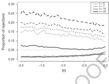
Proportion of rejections

Fig. 3 Comparison of the

proportion of rejections of uniformity using Sukhatme’s like method and the method described in Sect. 2

(for a detailed study of entropy, cf. [7]), whose graph is concave, and hence the 142

entropy of min#Xm Xp; 1#Xm 1#Xp $ _d D Xmp

6 is, for m; p 2 Œ!2; 2!, nearer to the entropy 143

of X0 than to the entropy of Xm and Xp. We would thus expect that Sukhatme’s 144

like method of sample augmentation would provide better results than the method 145

explained in Sect. 2. Observe however that further investigation of the matter seems 146

to indicate the reverse, as shown in Fig. 3 (the solid lines correspond to Sukhatme’s 147

like method and the dashed lines to the method described in Sect. 2). The general

AQ3 148

question of comparing analytically edfs of correlated samples remains unsolved, 149

even for simple forms of weak dependence only simulation results in well-defined 150

situations seem feasible. 151

Acknowledgements This research has been supported by National Funds through FCT— 152

Fundac¸˜ao para a Ciˆencia e a Tecnologia, project PEst-OE/MAT/UI0006/2011. The authors are 153

grateful to the referees for stimulating comments, leading to further results.

AQ4 154

References

1. Brilhante, M.F., Pestana, D., Sequeira, F.: Combining p-values and random p-values. In: 156

Luzar-Stiffler, V., et al. (eds.) Proceedings of the 32nd International Conference on Information 157

Technology Interfaces, pp. 515–520 (2010) 158

2. David, H.A., Nagaraja, H.N.: Order Statistics, 3rd edn. Wiley, New York (2003) 159

3. Deng, L.-Y., George, E.O.: Some characterizations of the uniform distribution with applications 160

to random number generation. Ann. Inst. Stat. Math. 44, 379–385 (1992) 161

4. Durbin, J.: Some methods of constructing exact tests. Biometrika 48, 4–55 (1961) 162

5. Gomes, M.I, Pestana, D., Sequeira, F., Mendonc¸a, S., Velosa, S.: Uniformity of offsprings 163

from uniform and non-uniform parents. In: Luzar-Stiffler, V., et al. (eds.) Proceedings of the 164

31st International Conference on Information Technology Interfaces, pp. 243–248 (2009) 165

6. Hartung, J., Knapp, G., Sinha, B.K.: Statistical Meta-Analysis with Applications. Wiley, 166

New York (2008) 167

7. Johnson, O.: Information Theory and the Central Limit Theorem. Imperial College Press, 168

UNCORRECTED

PROOF

8. Johnson, N.L., Kotz, S., Balakrishnan, N.: Continuous Univariate Distributions, vol. 2, 2nd 170

edn. Wiley, New York (1995) 171

9. Kulinskaya, E., Morgenthaler, S., Staudte, R.G.: Meta Analysis. A Guide to Calibrating and 172

Combining Statistical Evidence. Wiley, Chichester (2008) 173

10. Paul, A.: Characterizations of the uniform distribution via sample spacings and nonlinear 174

transformations. J. Math. Anal. Appl. 284, 397–402 (2003) 175

11. Pestana, D.: Combining p-values. In: Lovric, M. (ed.) International Encyclopedia of Statistical 176

Science, pp. 1145–1147. Springer, Heidelberg (2011) 177

12. Sequeira, F.: Meta-An´alise: Harmonizac¸˜ao de Testes Usando os Valores de Prova. PhD Thesis, 178

DEIO, Faculdade de Ciˆencias da Universidade de Lisboa (2009) 179

13. Sukhatme, P.V.: On the analysis of k samples from exponential populations with especial 180

UNCORRECTED

PROOF

AQ2. Please check if edit to sentence starting “Recently Paul [10] discussed....” is okay.

AQ3. Please check if edit to sentence starting “The general question...” is okay. AQ4. Picture given in the “Acknowledgement” has been deleted. Please check.